Partial Functional Linear Models with ARCH Errors

http://www.scirp.org/journal/ojs ISSN Online: 2161-7198

ISSN Print: 2161-718X

DOI: 10.4236/ojs.2018.82023 Apr. 26, 2018 345 Open Journal of Statistics

Partial Functional Linear Models

with ARCH Errors

Yafei Wang, Tianfa Xie, Zhongzhan Zhang

College of Applied Sciences, Beijing University of Technology, Beijing, China

Abstract

In this paper, the estimation of the parameters in partial functional linear models with ARCH(p) errors is discussed. With employing the functional principle component, a hybrid estimating method is suggested. The asymp-totic normality of the proposed estimators for both the linear parameter in the mean model and the parameter in the ARCH error model is obtained, and the convergence rate of the slope function estimate is established. Besides, some simulations and a real data analysis are conducted for illustration, and it is shown that the proposed method performs well with a finite sample.

Keywords

Asymptotic Normality, ARCH(p) Errors, Functional Principal Components, Convergence Rate, Least Absolute Deviation

1. Introduction

In order to combine the flexibility of linear regression models with the recent methodology for the functional linear regression models, partial functional linear models, which was introduced by [1], is considered as follows:

( ) ( )

d ,

Y = ′z+

∫

γ

t X t t+

ε



β

_(1.1)

where Y is a real-valued response random variable, z is a d-dimensional vector of random variables with zero means and finite second moments, and X t

( )

is an explanatory functional variable defined on  with zero mean and finite second moments (i.e.

( )

2

E X t < ∞, for all t∈ ), β is a d-dimensional vector

of unknown parameters, γ

( )

t is a square integrable function on , ε is a random error and is independent of z and X. For simplicity, without loss of generality, it is assumed that  =

[ ]

0,1 in the remainder of this paper. All the

random variables are defined on the same probability space

(

Ω,,P

)

. How to cite this paper: Wang, Y.F., Xie,

T.F. and Zhang, Z.Z. (2018) Partial Func-tional Linear Models with ARCH Errors. Open Journal of Statistics, 8, 345-361. https://doi.org/10.4236/ojs.2018.82023 Received: February 14, 2018

Accepted: April 23, 2018 Published: April 26, 2018

Copyright © 2018 by authors and Scientific Research Publishing Inc. This work is licensed under the Creative Commons Attribution International License (CC BY 4.0).

DOI: 10.4236/ojs.2018.82023 346 Open Journal of Statistics Model (1.1) has been studied by many authors from different points. From the view of estimation of model (1.1), for example, reference [2] studied the estimate of the model (1.1) using the nonparametric kernel regression methods and showed the proposed estimators are asymptotically normal as well as the estimator of the slope function γ

( )

t is consistent in supremum norm. Reference [3] considered the least square estimator of model (1.1) using the Karhunen-Loève (K-L) expansion to approximate the slope function, established asymptotic properties of the resulting estimation. Based on Tikhonov regularization, [4] introduced the functional ridge regression estimation procedure, and showed asymptotic normality of the estimated infinite dimensional regression coefficients as well as the convergence rate of the estimated slope function. Using the technique of polynomial splines, [5] considered the estimation of model (1.1) by minimizing the square of residuals, and furtherly considered the asymptotic property of the estimators. Recently, to get the robust estimator of coefficients of (1.1), the model has been also considered in the frame of qunatile regression ([6] [7]). Some authors also considered the model (1.1) from the view of hypothesis test, such as, [8] construct pivot by the square of residuals under the null and alternative hypothesis, to test whether the linearity term of (1.1) exists or not. Moreover, the generalized form of model (1.1), like semiparametric partially linear regression model for functional data and functional partial linear single-index model, has been respectively considered by [9][10].

However, all the works have a common assumption that the responses are observed independently. As is well known, uncertainty such as volatility uncertainty is a common phenomenon in modern economic and financial theory. Therefore, the assumption of independence of the response observations is not valid in the real data analysis. Motivated by the fact mentioned above, we may want to reconsider the model (1.1) so that it can reflect the volatility of the data. Fortunately, conditional heteroscedasticity can reflect the size of volatility approp- riately. One of the most popular models which can show the heteroscedasticity in econometrics is the autoregressive conditional heteroscedasticity (ARCH) model which was introduced by [11] and have had an enormous impact on the modeling of financial data. More importantly, many authors have studied the ARCH models to make it more perfect in theory. For example, reference [12] considered the existence of the strictly stationary and ergodic solution and high moment of the ARCH model; [13] studied strong law of large numbers of the absolute value sequence from ARCH.

If we have n observations

{

(

z1,X Y1, 1

)

,,

(

zn,X Yn, n

)

}

, model (1.1) can be

written as

( ) ( )

1

0 d .

i i i i

Y =

β

′z +

∫

γ

t X t t+

ε

(1.2)

The ARCH(p) model for

{ }

εi is defined by the following equations:

1 2

2 2 2

0 1 1 2 2

,

,

i i i

i i i p i p

e h

h

ε

α α ε

−

α ε

−

α ε

−

 = 

 _{= + + + +}

DOI: 10.4236/ojs.2018.82023 347 Open Journal of Statistics where α0 >0,αi ≥0,i=1,,p . Besides,

{

e ii: ≥1

}

is an independent and

identically distributed (i.i.d.) random sequence and independent of

{

ε_t:t<i

}

with Eei =0 and

2 ₁

i

Ee = . For sake of establishing the asymptotic properties of the joint model (1.2) and (1.3), in this paper, we assume that the distribution functions

{ }

Fi of

{ }

2

i

ε

are absolutely continuous with continuous densities

i

f , which is uniformally bounded away from 0 and ∞ at the 1/2-th quantile

points ξ =i,i 1,,n. Moreover, similar to [3], assume that

(

z1,X1

)

,,

(

zn,Xn

)

in (1.2) are i.i.d..

The ordinary regression models with ARCH errors have been considered by many authors. For example, [14] considered a p-th order autoregression process with ARCH errors; [15] studied the estimation of the partly linear regression models with ARCH(p) errors. Under some regularity conditions, we study the estimation of the unknown parameters in the joint model of (1.2) and (1.3), and propose a hybrid estimation method with combining the functional principle component analysis in the mean model with the least absolute deviation for the error model. The asymptotic normality of the real-valued parameter estimators is established, and the convergence rate of the slope function estimator is obtained.

The rest of the paper is organized as follows. Section 2 gives the estimation of parameters for the partial functional linear regression models as well as ARCH(p) errors. Asymptotic theory of the proposed estimators is given in Section 3. In Section 4, we carry out a simulation study to illustrate the finite sample performance, and a real data analysis is conducted in Section 5. Some preliminary lemmas and the proofs of the theorems are presented in Appendix.

2. Estimation

Firstly, we shall study how to produce the estimators βˆ ˆ,γ of β,γ in this

section. Let ⋅ ⋅, and ⋅ denote inner product and norm on 2

[ ]

0,1

L respectively. Denote the covariance function of process X by CX which is

continuous on  × . Then we have the following expansion

( )

( ) ( )

1

,

X j j j

j

C s t λ ρ s ρ t

∞

= =

∑

by Mercer’s theorem ([16]) with nonnegative eigenvalues λ λ1, 2, and

continuous orthonormal eigenfunctions ρ ρ1, 2, of the covariance operator.

For convenience, we assume λ λ1> 2 >>0 throughout this paper. Therefore,

by K-L expansion, one has

( )

( )

1

i ij j

j

X t U ρ t

∞

= =

∑

and

( )

( )

1

,

j j j

t t

DOI: 10.4236/ojs.2018.82023 348 Open Journal of Statistics where Uij = Xi,

ρ

j are uncorrelated random variables with E  = Uij 0 and

2

E_U_ij =

λ

_j, and

γ

_j =

γ ρ

, _j . Then (1.2) is equivalent to

1

, 1, , .

i i j ij i

j

Y γ U ε i n

∞

= ′

=β z +

∑

+ = (2.1)

To estimate the parameters in (1.2), following [3]’s idea, we approximate the second term in (2.1) by finite sum

1

, 1, , ,

m

i i j ij i

j

Y γ U ε i n

=

′ +z

∑

+ =

β

_(2.2)

where m→ ∞ as n→ ∞. Furthermore, we employ the empirical version of

X

C

( )

( ) ( )

( ) ( )

1 1

1

ˆ _, n _{ˆ ˆ ˆ}

X i i j j j

i j

C s t X s X t s t

n λ ρ ρ

∞

= =

=

∑

=

∑

with

(

ˆ_,ˆ

)

j j

λ ρ being the pairs of eigenvalues and eigenfunctions of covariance operator related to ˆ

X

C and λ λˆ₁≥ ˆ₂≥≥0, and substitute U_ij in (2.2) with

ˆ _,ˆ

ij i j

U = X

ρ

. To get an elegant matrix form for model (2.2), denote

(

Y1, ,Yn

)

′

=

Y , Z=

(

z₁,,z_n

)

′ ,

( )

_{1, ,}

1, ,

ˆ

m ij i n j m U ₌

=

=

U

,

(

1

)

, , _m

γ γ ′

=

γ _and

(

ε1, ,εn

)

′

=

ε . Then (2.2) can be rewritten as ,

m

+ +

YZβ U γ ε

and the least square estimator _βˆ _{and γ}ˆ _{are given by}

(

_{ˆ ,}ˆ

)

_{arg min}

(

) (

)

_.

m m

′ _′

′ ′ = Y−Z −U Y−Z −U

β γ β γ β γ

By simple calculation, we have

(

)

(

)

1

(

)

ˆ

m m

I − I Y

′ ′

= Z −V Z Z −V

β

with

(

)

1

m m m m m

−

′ ′

=

V U U U U and

(

)

1

(

)

ˆ ˆ

m m m

−

′ ′ = U U U Y−Z

γ β

provided that

(

(

)

)

1

m

I −

′ −

Z V Z exists (this is true with probability tending to 1,

see Lemma 1 in [8]). The estimator γˆ of γ can be given as

( )

( )

1

ˆ ˆ ˆ ,

m j j j

γ γ ρ

= ⋅ =

∑

⋅

where

γ

ˆ_j is the jth element of _γˆ_.

To get asymptotic properties of _βˆ_{, let} 1 1

ˆ n

i i i

Cz=n−

∑

₌ z z′,

1 1

ˆ n

i i i

CzY =n−

∑

₌ zY,

( )

1

( )

1

ˆ n

X i i i

Cz t =n−

∑

₌zX t , CˆX

( )

t

(

CˆX

( )

t

)

′ =

z z and

( )

( )

1 1

ˆ n

YX i i i

C t =n−

∑

₌Y X t .

Then _βˆ _{is equal to}

1

1 1

ˆ _{, ˆ} ˆ _,ˆ ˆ _,ˆ ˆ _{, ˆ}

ˆ ˆ ˆ _,

ˆ ˆ

m _{X j X j} m _{X j YX j}

Y

j _j j _j

C C C C

C C

ρ ρ ρ ρ

λ λ − = =         = − −     

∑

 

∑



z z z

z z

β _(2.3)

with 1

1

ˆ _{, ˆ} n _{, ˆ}

X j i i i j

DOI: 10.4236/ojs.2018.82023 349 Open Journal of Statistics larly,

γ

ˆ_j can be represented as _ˆ ˆ ˆ ˆ _,ˆ ˆ _{, 1, ,}

j CYX CX j j j m γ = −β′ _z ρ λ = .

So far, we have already obtained the estimator _βˆ _{and γˆ, now we turn to}

consider the estimation of

(

α α0, 1, ,αp

)

′

=

α . Denote by

1

ˆ ˆ

ˆ ˆ , 1, ,

m

i i i j ij

j

Y U i n

ε γ

= ′

= −β z −

∑

=

the residuals. For ARCH(p) models, in view of the higher peak and heavy tail phenomenon, unlike Sastry’s idea that regress _ˆ2

i

ε _{on a column of ones and} 2

1

ˆ_i

ε− by minimizing the sum of the square of residuals, after getting the residuals

ˆ ,i i 1, ,n

ε = to get the parameter’s estimate of ARCH (1) sequence ([14]), minimizing the sum of the absolute residuals is used in this paper to get an estimator of

(

α α0, 1, ,αp

)

′

=

α _{. That is to say}

1

2 2 2

0 1 1

1

ˆ arg min p ˆ ˆ ˆ ,

n

i i p i p

R i p

α_∈ + ε α α ε− α ε− = +

=

∑

− − − −

α _(2.4)

where ˆ

(

α αˆ0,ˆ1, ,αˆp

)

′

=

α .

3. Asymptotic Properties

We first state the assumptions under which the asymptotic properties are proved, then present the theorems. Let ρ

( )

D and _D⊗m denote the spectral radius and

Kronecker product of matrix D respectively, and _t =σ ε

{

_i:i≤t

}

in the following.

It is easy to see that E

[

εt|t−1

]

=0,

2 1

E

ε

t |t−  = ht, namely, the ARCH(p)

process forms a martingale difference sequence with 2 0 1

E

1

t

p

α

ε

α

α

  =

  _{− − −} . In order to attain the stationary solution and guarantee the existence of high moment of

{ }

εt , we suppose that

( )

0

1

0 , 1, 1

p

j r

j

α α ρ

=

< < ∞

∑

< Σ < _(3.1)

for some integer r≥1, where r E

( )

Dt r

⊗ Σ = _,

2 2 2

1 1

1 0 0

.

0 1 0

t p t p t

t

e e e

D

α α ₋ α

 

 

 

=  

 

 

 

Then, as [12] and [14] proved, there exists a strictly stationary solution for the p-th order ARCH process given by

1

2 2 2

0 1 1

1 0

j

t t t j t i

j i

e e D

ε α ∞ − − −

= =

 _′   = _ + _{  }

 



∑

δ

∏

δ  (3.2)

with δ1=

(

1, 0,, 0

)

′.

DOI: 10.4236/ojs.2018.82023 350 Open Journal of Statistics

4

E X < ∞

(3.3) and for each j

4 2

EUj ≤ C

λ

j (3.4)

for some constant C. For the eigenvalues of CX, assume that there exist C and

1

a> such that

1 1

1

, , 1

a a a

j j j

C− j− ≤λ ≤Cj− λ −λ₋ ≥Cj− − j≥

(3.5) to prevent the spacings among eigenvalues being too small. In order to guarantee that the regression weight function γ is smoother than the sample path X, for the Fourier coefficients

γ

j, we suppose that

b j Cj

γ

_≤ −

(3.6) for some constant C and b>a 2 1+ . On the tuning parameter, we assume that

( )

1 2

~ a b,

m n +

(3.7) where an~bn means there exist constants 0< <L M < ∞ s.t.

n n

a

L M

b

≤ ≤

for all n. Besides, we also assume that

4

d

R

E z < ∞

(3.8)

for the random vector z with

( )

1 2 d R = ′

z z z and Cz X_k

( )

⋅ =Cov

(

z Xk,

( )

⋅

)

satisfies

( )

,

k

a b z X j

C ρ ≤Cj− + (3.9) for each k=1, 2,,d and j≥1.

Let η_ik =z_ik− χ_k,X_i , where

(

)

1 k ,

k j Cz X j j j

χ ∞ ρ λ ρ

=

=

∑

_{. Then,}

1k, , nk

η η are i.i.d. random variables. We suppose that

[

]

2

1 1 1 1

E

η

k|X ,,Xn =0, E

η

k|X ,,Xn=Bkk, where Bkk is the kth diagonal element of

[

1 1

]

1

, , E X j X j ,

j j

C C

C ρ ρ

λ

∞ =

′

= = −

∑

z z z

B η η

(3.10)

which is assumed positive definite, and ηi=

(

ηi1,,ηid

)

′.

With the assumptions that mentioned above, we have the following results. Theorem 1. If the assumptions (3.1) with r=2, (3.3)-(3.10) hold, we have

(

)

1 2 0 1

1

ˆ _0,

1

d

p

n N α

α α −

 

− → _ _ − − −

 B 

β β

as n→ ∞, where “_→d _{” denotes convergence in distribution.}

Theorem 2. Under the assumptions (3.1) with r=1, (3.3)-(3.10), one has

( ) ( )

(

)

2 2 1 2

ˆ O_p n b a b .

γ γ_{− =} − − +

DOI: 10.4236/ojs.2018.82023 351 Open Journal of Statistics

2

r= , (3.3)-(3.10), we have

(

)

1 2 1 1

1 1

1

ˆ 0,

4

d

n − → N D PD− − _

 

α α

as n→ ∞, where

2 2 2

1 1

2 4 2 2 2 2

1 1

2 2 2 2 2 4

1 1 1 1 1

1

E ,

p p

p p p p p

p p

P

ε ε ε

ε ε ε ε ε ε

ε ε ε ε ε ε

− −

−

 

 

 

=  

 

 

 

( )

1 1

1

lim ,

n

n i i i i

i p

D →∞n− f ξ v v

= +

′

=

∑

with

(

2 2 2

)

1 2

1, , , ,

i p i p i i

v =

ε

+ −

ε

+ −

ε

′.

Remark 1. Compared with [3], we can find that the estimator of the regression coefficient vector also has the convergence rate n and is asympto-

tically normal under the ARCH(p) errors.

Remark 2. To implement the proposed method, we need to know how to choose the cut-off point m. Theoretically, if m is too large, the number of parameters in model (2.2) is also too large and the estimate of the slope function γ may goes terrible by the properties of Functional Principal Component Analysis (FPCA); if m is taken as a small value, the approximation of model (2.2) to model (2.1) may not be enough. This is the role that condition (3.7) plays. There are well-established methods for choosing such tuning parameter m, such as Generalized Cross-Validation (GCV), AIC, BIC and FPCA. As we all know, the first three criteria are data-driven and the FPCA is based on the ratio of variance explained by the first m eigenvalues to the total variation of X. In section 4, GCV and FPCA are respectively considered.

Remark 3. In order to make inference for α , the estimation of the asymptotic variance, mainly involving the estimation of P and fi

( )

ξi , is needed

to be given. Based on (A.8) in the Appendix, it is reasonable to use 1

1ˆ ˆ

n i i i p

n−

∑

_{= +}v v′ as the estimate of P with vˆi

(

1,

ε

ˆp i2+ −1,

ε

ˆ2p i+ −2, ,

ε

ˆi2

)

′

= . For fi

( )

ξi ,

the sparsity estimation methods or the kernel density estimation ideas, suggested by [17] and [18] respectively, can be used for this paper.

4. Simulation Studies

In this section, simulations are carried out to show the finite sample performance of the proposed method. The data is generated from the model (1.1) in the case where zi1 and zi2 are standard normal,

( )

200

( )

[ ]

1

, 0,1 ,

j j j

X t U ρ t t

=

=

∑

∈

where the Ujs are distributed as independent normal with mean 0 and variance

(

)

(

)

2

0.5 π

j j

λ = − − _{respectively,}

ρ

j

( )

t = 2 sin

(

(

j−0.5

)

πt

)

and

( ) ( )

1

1 1 2 2 ₀ d

i i i i i

DOI: 10.4236/ojs.2018.82023 352 Open Journal of Statistics with β =

(

2, 1 ,−

) ( )

′ γ t = 2 sin

(

π 2 3 2 sin 3π 2t

)

+

(

t

)

. For the random error, we take the following form: 1 2

i e hi i

ε = , 2 2

0 1 1 2 2

i i i

h =α +α ε₋ +α ε₋ , eii i d. . .~ t

( )

5 , where α0 takes value 0.1, α1 takes value from 0.1, 0.3 and α2 takes value

from 0.3, 0.1 correspondingly. Note that t

( )

5 has finite 4th order moment, and

the condition (3.1) is satisfied by α=

(

0.1, 0.1, 0.3

)

′ and α=

(

0.1, 0.3, 0.1

)

′

with r=1, where it may be shown that both βˆ and αˆ given by (2.3) and

(2.4) are consistent. For α=

(

0.1, 0.3, 0.3

)

′ with r=1, ρ

( )

Σ =_r 1. That is, it is

on the boundary of the condition region.

We also consider the situation that α1 and α2 take values 0 to compare

with the independent structure. For each α, we simulate 1000 random samples, each with sample size n=100, 300, 500 respectively. For the determination of

m by FPCA,

{

1 1

}

ˆ ˆ min : k _i n _i 0.85

i i

m= k

∑

₌λ

∑

₌λ ≥ is used. The accuracy of the slope function estimate is checked by the mean integrated square error (MISE) which is defined as

( ) ( )

(

)

1000

2

1 1

1 1

ˆ

MISE ,

1000

N

i s s

i s

t t

N

γ

γ

= =

 

= _ − _

 

∑ ∑

where γˆ_i

( )

⋅ is the estimate of the slope function γ

( )

⋅ obtained from the i-th

[image:8.595.208.540.496.720.2]

replication, and t ss, =1,,N are the equally spaced grid points at which the function γˆ_i

( )

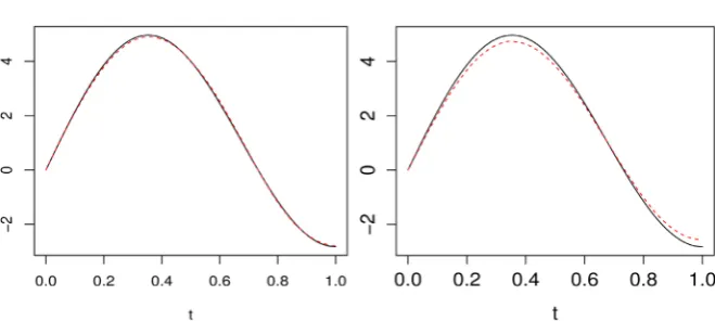
t is evaluated. In our implementation, N =100 is used. In this section, the results of the estimators of α using the Least Square (LS) method is also carried out to compare with the Least Absolute Deviation (LAD) method which is proposed by this paper. The results are summarized into Tables 1-3 and the shape of the true function γ and the estimated function γˆ, based on the average of 1000 replications with α=

(

0.1, 0.1, 0.3

)

′ are depicted in Figure 1.

Table 1. MSE and MISE under LAD (GCV).

n (α α1 2) β1 β2 γ α0 α1 α2

[image:9.595.209.539.89.259.2]

DOI: 10.4236/ojs.2018.82023 353 Open Journal of Statistics

Table 2. MSE and MISE under LAD (FPCA).

n (α α1 2) β1 β2 γ α0 α1 α2

[image:9.595.208.539.292.461.2]

100 (0.1 0.3) 0.0056 0.0059 0.6424 0.0028 0.0096 0.0464 (0.3 0.1) 0.0054 0.0066 0.6453 0.0031 0.0465 0.0086 (0.3 0.3) 0.0164 0.0176 0.8812 0.0094 0.0480 0.0491 300 (0.1 0.3) 0.0017 0.0019 0.0910 0.0022 0.0053 0.0362 (0.3 0.1) 0.0017 0.0017 0.0911 0.0022 0.0351 0.0061 (0.3 0.3) 0.0059 0.0084 0.2079 0.0021 0.0382 0.0416 500 (0.1 0.3) 0.0009 0.0009 0.0581 0.0022 0.0041 0.0318 (0.3 0.1) 0.0010 0.0009 0.0573 0.0021 0.0311 0.0050 (0.3 0.3) 0.0030 0.0030 0.1284 0.0020 0.0357 0.0399

Table 3. MSE and MISE under LS (GCV).

n (α α1 2) β1 β2 γ α0 α1 α2

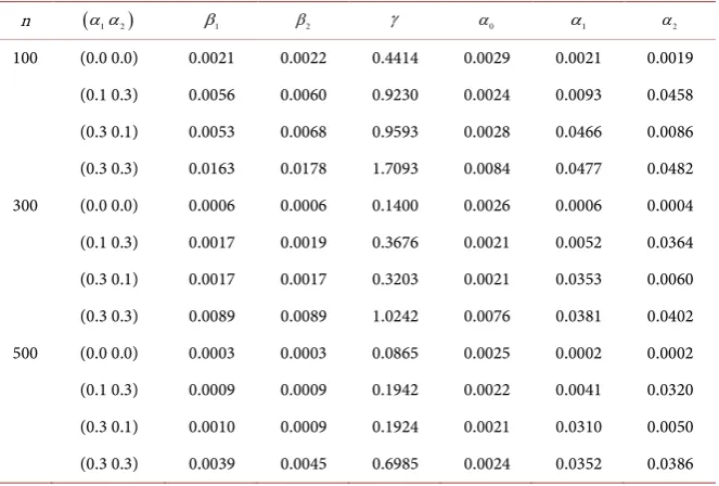
100 (0.1 0.3) 0.0056 0.0060 0.9230 0.1559 0.0203 0.0411 (0.3 0.1) 0.0053 0.0068 0.9593 0.1286 0.0412 0.0252 (0.3 0.3) 0.0163 0.0178 1.7093 4.1482 0.0430 0.0541 300 (0.1 0.3) 0.0017 0.0019 0.3676 0.1011 0.0122 0.0258 (0.3 0.1) 0.0017 0.0017 0.3203 0.0619 0.0271 0.0206 (0.3 0.3) 0.0089 0.0089 1.0242 25.1315 0.0318 0.0690 500 (0.1 0.3) 0.0009 0.0009 0.1942 0.1215 0.0123 0.0230 (0.3 0.1) 0.0010 0.0009 0.1924 0.1684 0.0259 0.0251 (0.3 0.3) 0.0039 0.0045 0.6985 18.6453 0.0305 0.0525

Table 4. MSE and MISE with N

( )

0,1 produced errors under GCV (α=

(

0.1, 0.3, 0.3

)

′).

n β1 β2 γ α0 α1 α2

100 LAD 0.0030 0.0028 0.6190 0.0027 0.0455 0.0473 LS 0.0030 0.0028 0.6190 0.0049 0.0379 0.0472 300 LAD 0.0009 0.0009 0.1982 0.0028 0.0373 0.0387 LS 0.0009 0.0009 0.1982 0.0023 0.0201 0.0261 500 LAD 0.0006 0.0005 0.1088 0.0029 0.0341 0.0345 LS 0.0006 0.0005 0.1088 0.0022 0.0171 0.0220

We also would like to know that how will the LAD method behave when the error of the ARCH sequence is not heavy tailed, such as e~N

( )

0,1 . The

simulation results are summarized into Table 4 with α=

(

0.1, 0.3, 0.3

)

′. In this

case, (3.1) is satisfied with both r=1 and r=2.

We can derive the following conclusions from Tables 1-4.

[image:9.595.207.540.500.620.2]

DOI: 10.4236/ojs.2018.82023 354 Open Journal of Statistics seen MSEs, MISE decrease in all scenarios that we considered about error. This reflects the proposed estimators fit better to the real values as the sample size increases and thus is promising.

2) For every fixed sample size n, it can be seen the larger value of coefficients α, the larger the corresponding MSE for the different coefficients form of errors. For example, when n=100, α take values

(

0.1, 0.1, 0.3

)

and

(

0.1, 0.3, 0.1

)

respectively, the MSE of α =1 0.3 is larger than the MSE of α =1 0.1 and so is 2

α _{. Moreover, the MSE of} αˆ and MISE of γˆ become large when the coefficients α α1, 2 take relative large values simultaneously, such as

(

α α1, 2

) (

= 0.3, 0.3

)

in Table 1. This is due to the stronger volatility for larger

, 1, 2

j j

α

= _.

3) From Table 1, for every fixed sample size n, when α α1, 2 take values 0,

which is the case considered by [3], the MSE and MISE of _βˆ _{are smaller than}

those with ARCH errors. This shows that the dependence of errors makes the estimators more varying. However, with the increasing of sample size, the later ones decrease and could reach the former quantities.

4) The MSE of the coefficients αˆ, in Table 3, using the LS method for t

( )

5

produced errors get larger values, compared to the results of estimator given by (2.3). Specifically, unlike the results in Table 1 and Table 2, the results of α0

for the boundary case

(

α α1, 2

) (

= 0.3, 0.3

)

are unstable, illustrating the reasona- bleness of the proposed method.

5) Table 4 shows that the LAD method could perform as well as the LS method even for non-heavy tailed distribution of the error.

6) As Table 1 and Table 2 show, the difference of the estimators of β

between the two selection methods of m is very small.

Based on simulation results from Table 1 and Table 2, it seems that the estimator of

γ

corresponding to FPCA is better in view of MISE. As we know, when using FPCA to choose m, a threshold value for the ratio is needed. We reset the threshold value as 0.80 rather than 0.85 for the case n=100 and

(

0.1, 0.1, 0.3

)

′

=

α , the MISE will become 6.6373 which is bigger than 0.9230

given in Table 1. As far as we know, there is no theoretical research on how the threshold value should be set to get a compromise between goodness of fit and the precision of the estimated slope function.

From Figure 1, it can be seen that the estimated function can fit the true function approximately no matter which method is used to choose the tuning parameter m, which demonstrate that the proposed method works well.

From the above observation, we see that the estimator (2.4) performs well, even under the boundary condition. It may be theoretically interesting to know the performance of the estimator in this case, but it is beyond our focus here.

5. Real Data Analysis

[image:11.595.209.539.61.209.2]

DOI: 10.4236/ojs.2018.82023 355 Open Journal of Statistics

Figure 1. The true function γ (solid line) and the estimated function γˆ (dashed line)

using GCV (left) and FPCA (right) with n=100.

commercial sectors from January 1972 to January 2005 (397 months) and their annual average retail price P (33 years). A main goal of this study is to consider the effect of dependence structure of the error on the asymptotic variance of _βˆ_,

when using the price and consumption to predict the consumption 6 months later.

According to the stationary test of the electricity consumption data, the heteroscedasticity and linear trend can be found and then may be eliminated by differencing the ln data. Corresponding to the general notation introduced in model (1.1), let

1

ln ln , 1, 2, ,397,

j j j

D = C − C₋ j=

( )

[

]

{

12 1 , 1,12 ,

}

1, 2, , 32.

i i t

X = D _{− +} t∈ i= The response variable is

12 6, 1, 2, , 32,

i i

Y =D + i=

and the additional real variable is defined by , 1, 2, , 32.

i i

z =P i=

[image:12.595.232.520.69.331.2]

DOI: 10.4236/ojs.2018.82023 356 Open Journal of Statistics

[image:12.595.246.503.378.603.2]

Figure 2. The graph of error sequence.

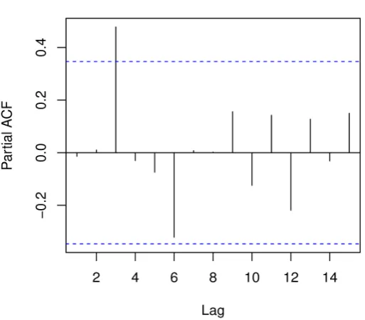
Figure 3. The pacf of the errors square.

of _βˆ _{is 0.01, which is reduced by 94% comparing with the value 0.18, which is}

given under ignoring concrete form of the error, showing it is promising to consider the ARCH structure.

6. Discussion

DOI: 10.4236/ojs.2018.82023 357 Open Journal of Statistics errors using the LS method, as well as the parameters of ARCH(p) sequence using the LAD method are respectively considered. Considering that the dimensionality of the slope function is infinite, for this paper, the key point we have given consists in transforming the partial functional linear models with ARCH errors into the corresponding linear regression models by the K-L expansion and the idea of FPCA. The linear relationship between z and X is essentially assumed (see Remark 1 in [8]). In the future study, under the errors’ dependent structure, we will further consider the estimation of the model (1.1) using the kernel method noticing that the relationship between z and X may be relaxed. Since the heteroscedasticity in economics is a common phenomenon, the theory study of the model is practically useful and worthy to be explored. Furthermore, based on the fact the consistency of αˆ and _βˆ _{can be}

respectively obtained from Theorem 3 and the proof of Theorem 1, the inference to the models could be made precisely within this paper by the asymptotic normality of _βˆ_.

Acknowledgements

This work is supported by NSFC No. 11771032, No.11571340 and the Science and Technology Project of Beijing Municipal Education Commission No. KM201710005032.

References

[1] Aneiros-Pérez, G. and Vieu, P. (2006) Semi-Functional Partial Linear Regression. Statistics & Probability Letters, 76, 1102-1110.

https://doi.org/10.1016/j.spl.2005.12.007

[2] Aneiros-Pérez, G. and Vieu, P. (2008) Nonparametric Time Series Prediction: A Semi-Functional Partial Linear Modeling. Journal of Multivariate Analysis, 99, 834-857. https://doi.org/10.1016/j.jmva.2007.04.010

[3] Shin, H. (2009) Partial Functional Linear Regression. Journal of Statistical Planning and Inference, 139, 3405-3418. https://doi.org/10.1016/j.jspi.2009.03.001

[4] Shin, H. and Lee, M. (2012) On Prediction Rate in Partial Functional Linear Regres-sion. Journal of Multivariate Analysis, 103, 93-106.

https://doi.org/10.1016/j.jmva.2011.06.011

[5] Zhou, J.J., Chen, Z. and Peng, Q.Y. (2016) Polynomial Spline Estimation for Partial Functional Linear Regression Models. Computational Statistics, 31, 1107-1129.

https://doi.org/10.1007/s00180-015-0636-0

[6] Lv, Y., Du, J. and Sun, Z.M. (2014) Functional Partially Linear Quantile Regression Model. Metrika, 77, 317-332.

[7] Zhou, J., Du, J. and Sun, Z.M. (2016) M-Estimation for Partially Functional Linear Regression Model Based on Splines. Communications in Statistics-Theory and Me-thods, 45, 6436-6466. https://doi.org/10.1080/03610926.2014.921309

[8] Yu, P., Zhang, Z.Z. and Du, J. (2016) A Test of Linearity in Partial Functional Li-near Regression. Metrika, 79, 953-969. https://doi.org/10.1007/s00184-016-0584-x

DOI: 10.4236/ojs.2018.82023 358 Open Journal of Statistics 2518-2529. https://doi.org/10.1016/j.jspi.2012.03.004

[10] Wang, G.C., Feng, X.N. and Chen, M. (2015) Functional Partial Linear Single-Index Model. Scandinavian Journal of Statistics, 43, 261-274.

[11] Engle, R.F. (1982) Autoregressive Conditional Heteroscedasticity with Estimates of United Kingdom Inflation. Econometrica, 50, 987-1007.

https://doi.org/10.2307/1912773

[12] Chen, M. and An, H.Z. (1995) The Strictly Stationary Ergodicity and High Moment of ARCH(p) Models. Chinese Science Bulletin, 40, 2118-2123.

[13] Zhang, Z.Q., Feng, J.Y. and Zhang, R.Q. (2007) Strong Law of Large Numbers of the Absolute Value Sequences from ARCH. Journal of Yanbei Normal University, 23, 9-11.

[14] Sastry, G.P. (1988) Estimation of Autoregressive Models with ARCH Errors. The Indian Journal of Statistics Series B, 50, 119-138.

[15] Lu, Z.D. and Gijbels, I. (2001) Asymptotics for Partly Linear Regression with De-pendent Samples and ARCH Errors: Consistency with Rates. Science in China Se-ries A: Mathematics, 44, 168-183. https://doi.org/10.1007/BF02874419

[16] Riesz, F. and Sz-Nagy, B. (1955) Functional Analysis. Dover Publications, New York.

[17] Hendrick, W. and Koenker, R. (1991) Hierarchical Spline Models for Conditional Quantiles and the Demand for Electricity. Journal of the American Statistical Asso-ciation, 87, 58-68. https://doi.org/10.1080/01621459.1992.10475175

[18] Pollard, D. (1991) Asymptotics for Least Absolute Deviation Regression Estimators. Econometrics Theory, 7, 186-199. https://doi.org/10.1017/S0266466600004394

[19] Revesz, P. (1968) The Laws of Large Numbers. Academic Press, New York. [20] Hall, P. and Heyde, C.C. (1980) Martingale Limit Theory and Its Application.

Aca-demic Press, New York.

[21] Pollard, D. (1984) Convergence of Stochastic Process. Springer-Verlag, New York.

https://doi.org/10.1007/978-1-4612-5254-2

[22] Bosq, D. (2000) Linear Processes in Function Spaces. Springer-Verlag, New York.

https://doi.org/10.1007/978-1-4612-1154-9

[23] Koenker, R. (2005) Quantile Regression. Cambridge University Press, Cambridge.

DOI: 10.4236/ojs.2018.82023 359 Open Journal of Statistics

Appendix

. Proofs of the Theorems

We will state the proofs of the theorems given in Section 3. Firstly, some lemmas will be given.

Lemma A.1. ([12], Theorem 1)

{ }

εt is a strictly stationary solution of model

(1.3) and 2 0

Eε < ∞ if and only if

∑

p_j=1α_j<1. Furthermore, this solution is

unique and ergodic.

Lemma A.2. ([12], Theorem 3) Let

( )

{

1

}

E , is random variable

r r r

r

L = x x = x < ∞ x and suppose (3.1) holds,

( )

4 1

Ee_t r− < ∞, where r≥1 is an integer, then εt2∈Lr.

Lemma A.3. Consider

{

εi:i≥1

}

forms an ARCH(p) process. Besides, (3.1)

holds, then

1 2 2

1

E . .

n

r r

i i

i

n− ε ε a s

=

  →  

∑

for the integer r in condition (3.1); furthermore, if r≥2, then

1 2 2 2 2

1

E a.s..

n

i i j i i j i

n− ε ε₋ ε ε₋

=

  →  

∑

Proof. From Lemma A.1 and the representation (3.2), it follows that

{ }

εt

and

{ }

2

t

ε

_{are strictly stationary ergodic sequences. Combining with Lemma A.2,}

the results follow immediately from the ergodic theorem ([19][20]).

Lemma A.4. If ε is independent of X and (3.1)-(3.2) hold, one has 1

1 2

1

.

n

i i p i

n− Xε O n−

=

  = _ _  

∑

Proof. By simple calculation, the conclusion can be easily derived under the

fact 2

(

)

0 1

E  = 

ε

i

α

1−

α

− −

α

p .

Proof of Theorem 1. Let

( )

1

(

)

ˆ ˆ ˆ _{,ˆ ˆ ,}

k m

k x j= Cz X ρj λj ρj x

Φ =

∑

and

( )

1

(

k ,

)

,

k x j Cz X ρj λj ρj x

∞ =

Φ =

∑

_with 2

(

[ ]

)

0,1

x∈L . Set

max_{i j ij}

A_∞=

∑

A and

1 1

d d ij i j

A =

∑ ∑

_{= =} A for A

( )

Aij Rd d

×

= ∈ _{. Observe that}

(

)

(

)

1 2 1 1 2

1 =1

1 1 2

1 1

1 1 1

1 1

ˆ _{,ˆ ,ˆ} 1

ˆ ˆ _,

ˆ ˆ _{,ˆ ,ˆ}

ˆ _,

ˆ

ˆ _{, ˆ , ˆ}

, ,

ˆ

n m _{X j i j}

i i i

i j _j

n m

X j i j

i i

i j _j

n m _{X j i j}

X j i j

i

i j j j j

n i

i j

C X

n n X

n C X n X C X C X C ρ ρ γ ε λ ρ ρ γ λ ρ ρ ρ ρ ε λ λ − = − − = = ∞ = = = ∞ = =      _{ }  − =  _ − _ +   _{ }          = _{ } −          + −     + −

∑

∑

∑

∑

∑ ∑

∑

∑

∑

z z z z B z B z z β β , ,

X j i j

DOI: 10.4236/ojs.2018.82023 360 Open Journal of Statistics

with

{

( )

}

, 1, ,

ˆ ˆ

ˆ ˆ

m

k z X

k m d

C C

= = z− Φ

B

.

According to Lemma A.4, similar to [3], one has

( ) ( )

(

2 1 2

)

ˆ b a b _, p

O n− − +

∞ − = B B

( )

1 2 1 1

ˆ _{,ˆ ,ˆ}

, 1 , ˆ

n m _{X j i j}

i i p

i j _j

C X

n X o

ρ ρ γ λ − = =    ₋  ₌    

∑

∑

z

z

( )

1 2

1 1 =1

ˆ _{,ˆ ,ˆ} , ,

1 . ˆ

n m _{X j i j}

X j i j

i p

i j j j j

C X C X n o ρ ρ ρ ρ ε λ λ ∞ − = =    ₋  ₌    

∑ ∑

z

∑

z

Now, we consider the term

1 2 1 2

1 1 1

, ,

:

X j i j

n n

i i i i

i j i

j

C X

n ρ ρ ε n ε

λ ∞ − − = = =    −  =    

∑

∑

z

∑

z η . We will show

1 2 0

1 1 0, . 1 n d i i i p

n ε N α

α α − =   → _ _ − − −  

∑

B

η (A.1)

Let Pj−1

( )

⋅ =E |⋅ j−1 and i n1 2 i iε

−

=

ξ η _{, then}

_{{ }}

ξ_{i forms a martingale} difference series due to the fact that ξi is i−1-measurable and Pi−1

( )

ξi =0.

Let ui denote the conditional variances of ξi, then, for i=1,,n,

( )

1

(

2

)

1

(

)

( )

2 1

1 1 E 1 .

i i i i n i i i i

ε

n i i i

ε

i n hi

− − −

− ′ − ′ ′ −

= = = =

u P

ξ ξ

P

ηη

ηη

P B

Therefore, 1 0 1 , 1 p i i

i i p

n h

α

α

α

−

= →

− − −

∑

u

∑

B B

according to the law of large numbers ([19]). Furthermore, for any

δ

>0,

{

}

(

)

{

}

(

)

{

}

{

}

( )

(

{

}

)

{

}

(

)

(

)

1

1 2 1 2

1

2

1 2 1 2 2 1 2

1

2

1 2 1 2

1 1 1 1

1 2 2 1 2

1 E 1 1 .

j j j j j

j j j j j j j

j j j j j j

j

j j j

j j j j

n P n

n n n

n E n

n n

δ

ε ε δ

ε δ ε δ

ε δ

ε ε δ

− − − − − − − − − ′ > ′ = >  _′  

≤ _{ } > > _

    ′ = > ′ + >

∑

∑

∑

∑

∑

P P P P ∪ ξ ξ ξ

η η η

η η η

η η η

η η

For the first term, it converges to zero because

η η

j ′j is uniformly integrable.

In view of the integrability of 2

i

ε , the second term also converges to zero in probability. Using the martingale difference central limit theorem (CLT) ([21], we get (A.1) holds. Therefore, the conclusion of Theorem 1 holds.

Proof of Theorem 2. With Lemma A.4, the technics in the proof of Theorem 3.2 of [3] can be extended to the present model. So we omit it here.

DOI: 10.4236/ojs.2018.82023 361 Open Journal of Statistics 1

1 2 1 2 2

1 1

ˆ ,

n n

i i p

i p i p

n− ε n− ε o n−

= + = +

  = + _ _  

∑

∑

(A.2)

1

1 2 2 1 2 2 2

1 1

ˆ ˆ .

n n

i i j i i j p

i p i p

n− ε ε₋ n− ε ε₋ o n−

= + = +   = + _ _  

∑

∑

(A.3) From Theorem 1 and Theorem 2, we learn that

(

)

2 2

(

(_{2 1}) ( ₂ )

)

1

ˆ

ˆ ,

m

b a b

j j p

j

O n

γ γ − − +

=

− = − =

∑

γ γ

_(A.4)

( )

1 2

ˆ _.

p O n−

− =

β β

(A.5) Under the conditions (3.5)-(3.7) and _X∈L2

( )

_ , one has

( ) ( )

(

)

2 2 _{2 1 2}

2 2

1 1

, b , b a b .

j i j i j p

j m j m

X C j X O n

γ ρ ρ

∞ ∞ − − + − = + = + ≤ =

∑

∑

(A.6) In addition, according to (3.3) and λ λ1> 2>>λm, the relation

2

ˆ lim sup E j j

n

n ρ ρ

→∞ − < ∞ (A.7) holds, see ([22], ch4). For the residual _ˆ2

i

ε _{, we have}

(

)

(

)

1 1 1 1 1 1 ˆ ˆ ˆ ˆ

ˆ _ˆ ˆ

ˆ _{ˆ , ˆ}

ˆ

, ,

m

i i i j ij

j

m

i j ij i i j ij

j j

m

i i j j i j

j m

j i j j j i j

j j m

Y U

U U

X

X X

ε γ

γ ε γ

ε γ γ ρ

γ ρ ρ γ ρ

= ∞ = = = ∞ = = + ′ = − − ′ ′ = + + − − ′ = − − − − − − +

∑

∑

∑

∑

∑

∑

z z z z β β β β β

by (2.1). Combining this equality with (A.4)-(A.7), (A.2) and (A.3) can be proved.

Now we turn to consider the asymptotic form of αˆ. By Lemma A.3, we can conclude

(

)

1

1_{ˆ ˆ} 1 _{. . as ,}

n P P− ′ − →P− a s n→ ∞ (A.8) where

2 2 2

1 1

2 2 2

1 2

2 2 2

1 2

ˆ ˆ ˆ 1

ˆ ˆ ˆ 1

ˆ _.

ˆ ˆ ˆ 1

p p

p p

n n n p

P

ε ε ε

ε ε ε

ε ε ε

− + − − −       =        

Combine (A.2), (A.3), (A.8) and the assumptions about the densities of

{ }

2

i

ε

_,