ISSN Online: 2164-5175 ISSN Print: 2164-5167
A Study on the Balanced Assignment of
Allocating Large Group with Multiple Attributes
into Subgroups
*
Young Rhee
Department of Industrial and Management Engineering, Keimyung University, Taegu, South Korea
Abstract
In this paper, a balanced assignment methodology is proposed in case of enti-ty with more than 2 attributes. The Mahalanobis distance is a basic idea of MTS method as a distance indicator considering the correlation of entities in quality control techniques. This can be applied to ensure the balanced as-signment, and utilized the Signal to Noise Ratio as a measure of classifying large groups with entities into many subgroups. In order to analyze the ba-lanced assignment, the simulation is performed for a given example. Valida-tions against simulation data establish the effectiveness of this approach.
Keywords
Balanced Assignment, Mahalanobis Distance, Signal to Noise Ratio, MTS
1. Introduction
Decision making process with multi-attributes is different from the well-known solution methodology, but the efforts are being made to improve it due to the difficulty of the optimization process. A mathematical model or an application methodology with a constraint such as a series of processes for finding an ap-propriate compromise among attributes that are in conflict with each other is modeled as a multi-criteria function, and its necessity is increasing. Among the methods of solving the multi-criteria function, the most commonly used ap-proaches are the weighting method and the goal programming method. In the optimization process, weights or specific numerical goals should be set appro-priately for each function using the mathematical programming approaches.
*The present research has been conducted by the Sabbatical Research of Keimyung University in 2016.
How to cite this paper: Rhee, Y. (2018) A Study on the Balanced Assignment of Al-locating Large Group with Multiple
Attributes into Subgroups. American
Jour-nal of Industrial and Business Manage-ment, 8, 1418-1432.
https://doi.org/10.4236/ajibm.2018.86095
Received: May 4, 2018 Accepted: June 4, 2018 Published: June 7, 2018
Copyright © 2018 by author and Scientific Research Publishing Inc. This work is licensed under the Creative Commons Attribution International License (CC BY 4.0).
http://creativecommons.org/licenses/by/4.0/ Open Access
However, if the parameter is wrongly selected, the burden of not obtaining the Pareto optimal solution certainly exists.
In the meantime, as a mathematical approach to multi-criteria problems, the constrained problem by using the distance and fuzzy measure is solved by Bar-ron and Schmidt [1]. For the more complicated model, Dyer and Sarin [2], and French [3] have proposed some approaches to solve this problem through the kinds of surveys, but the mixture of alternatives and attributes give rise to nu-merous solutions, which led to the question of the solution tracking. Since then, the well-known MTS (Mahalanobis Taguchi System) method has been intro-duced [4] [5]. The MTS method is to utilize the distance between an entity and the special space of the data group, that is, the Mahalanobis distance, by analyz-ing the characteristics of the attributes inherent in each entity without requiranalyz-ing any parameter setting. In other words, the MTS method defines the Mahalanobis space as unit space in multi-dimensional spaces and calculates how far an entity is from this space.
Clustering or assignment is one of the ways to classify large groups with many entities into many subgroups according to the given criteria. Clustering means a grouping method based on attributes of each entities and certain criteria, and the similarity among entities plays an important role. For example, if a group of students is divided into two groups based on height 180 centimeter, tall group and non-tall group, based on so called height attribute, a group is classified into a tall subgroup and a non-tall subgroup. And the classified two small groups are made a new characteristic, such as beanpole group and ordinary group.
In this study, the properties inherent in an entity are defined as attributes, and the properties representing a group are defined as characteristics. On the other hand, the assignment is a grouping method considering each attribute according to the purpose of subdividing them into many subgroups. The balanced assign-ment is a grouping method by matching the mean or variance of the attributes to make each subgroup similar. Therefore, the characteristics of the subgroup are disappearing. It is not difficult to solve the problem of the balanced assignment in case of an entity with less than or equal 2 attributes. However, to solve the ba-lanced assignment problem where an entity has more than or equal to 3 attributes, is somewhat complicated, but various solution approaches can be proposed. In order to reduce the interaction due to the attribute in the entity which conflicts with each other, the first step is to simplify to the similar attributes taking into account the correlation between attributes, and it is a sim-ple and surprisingly good way to expect good results. Secondly, to apply the suitable weights for each attribute is recommended as a good approach. Since the determination of weight is key issue, the opinions of experts in the field are required to estimate the weight.
In this study, the Mahalanobis distance instead of the Euclidean distance is applied to ensure the balanced assignment, and the SNR (Signal to Noise Ratio) is utilized as a measure of classifying large groups with many entities into sub-groups. The Mahalanobis distance is a basic idea of the MTS method as a
tance indicator considering the correlation of entities in quality control tech-niques. In addition, the SNR indicates the influence of each entities correspond-ing to the Mahalanobis space.
The paper is organized as follows. We review related work in Section 2. And the concept of balanced assignment is introduced in Section 3. In Section 4, an example to allocate multiple entities into many subgroups is presented and the result of the MTS method is checked by comparing it against the simulation re-sult. Finally, Section 5 gives concluding remarks.
2. Related Studies
The solving approach to the balanced assignment is applying a special case of the well known clustering methodology. In this section, the MTS-related studies are introduced for the purpose of classifying large groups with multiple attributes into many subgroups.
2.1. Clustering
Clustering algorithm is an algorithm that aggregates similar entity without prior knowledge of the entity. That is, after measuring the degree of similarity among entity, the classification is performed so as to form a cluster among the entity having the highest degree of similarity. Completing the classification by cluster-ing, the similarity of the entity in the group is maximized, and the similarity be-tween the groups is minimized. On the other hand, the classification by the ba-lanced assignment results in that the similarity of the entity in the group is mi-nimized and the similarity between the groups is maximized. The nearness be-tween the entities is usually measured by the specific distance measure such as the Mahalanobis distance and Euclidean distance [6].
The clustering methodologies can be divided into hierarchical, density based, grid based, and model based methods. The hierarchical method is a method of hierarchically classifying and clustering a given set of entities using the tree structure, and there are a bottom-up method and a top-down method. A density based method is about forming clusters based on density, which provides an ef-ficient clustering method for objects with multidimensional and spatial attributes. The grid based method divides a set of entities into a finite number of cells to form a structure, and all clustering operations are performed on this grid structure. Since the performance of this method depends on the number of di-vided cells in each dimension, the time efficiency decreases as the dimensionality increases and the number of cells increases. Finally, the model-based method is a method that finds the optimal combination between the model and the given entity using a special mathematical model.
2.2. Mahalanobis Distance
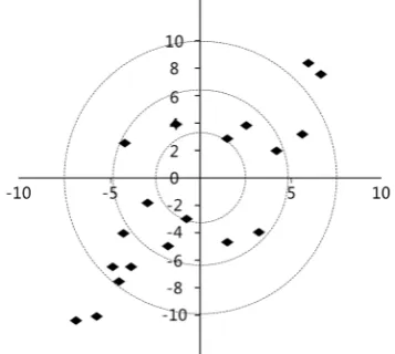
The Euclidean distance as shown in Figure 1, which is often used as a distance measure of the space concept, is applied under the assumption that the properties
Figure 1. Euclidean distance.
of the attributes that an object is inherent are consistent. The Euclidean distance is defined as the shortest distance connecting two points. For example, the distance of two points A (x1, y1) and B (x2, y2) in two dimensions is expressed as
(
) (
2)
21 2 1 2
AB
ED = x x− + y y− . Simply, this is a basic distance measurement in which the correlation between attributes is not considered.
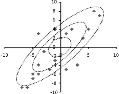
On the other hand, the Mahalanobis distance is already known as an effective way to simply compare between groups with well-known characteristics and those who are not familiar with the characteristics [5]. Characteristically, the Mahalanobis distance is calculated by taking into account the correlation of va-riables as a measure of the degree of dispersion of vava-riables. Since the Mahala-nobis distance is very sensitive to standardized variables, it leads to a large in-creasement, even though the standardized variable is slightly different for the reference group [3]. Applying this to all attributes on the entity, the Mahalanobis distance can be readjusted by considering the correlation between attributes. The description of the Mahalanobis distance is shown in Figure 2.
As seen in Figure 1, the Euclidian distance has the form of a circle, since it does not take into account the correlation between attributes. On the other hand, the Mahalanobis distance takes the form of an ellipse in consideration of the correlation, and is expressed as follows.
(
) (
1)
t 1/2rs r s r s
MD = x −x S− x −x
(1)
In (1), MDrs denotes the Mahalanobis distance between entity r and entity s. And also S−1 denotes the inverse matrix of the covariance, and
(
)
tr s
x −x is
expressed as the transpose matrix of
(
xr−xs)
.The difference between the Euclidean distance and the Mahalanobis distance is that the Euclidean distance is used when all attributes are measured in the same unit and are independent. On the other hand the Mahalanobis distance is applied the covariance matrix as a multivariate measure based on the correlation between attributes. The Mahalanobis distance is effective when the units of attributes are different and there exist the correlation between attributes.
Figure 2. Mahalanobis distance.
2.3. Orthogonal Array Table
The orthogonal array table is designed to be able to model experimental designs that can reduce the number of experiments. In experimental design, many fac-tors need to be considered in order to reduce product defects or to minimize the dispersion of quality, so that the orthogonal array table can be usefully accessed in this environment. The orthogonal array table detects the main effects and the two-factor interactions, which seem to be technically feasible in case of large number of factors, and reduce the number of experiments at the expense of high-order interactions, which seem technically absent. The orthogonal array ta-ble has some advantages of ease deployment such as fractional factorial design, split-plot design, compounding method etc., while reducing the number of ex-periments. And it helps easy to calculate the factorial variation and can includes many factors without scaling-up the experimental design itself.
In general, 2-level orthogonal array table and 3-level orthogonal array table are used the most, even though the orthogonal array table has 2, 3, 4, 5 level sys-tem and mixed level syssys-tem. The orthogonal array table of the two-level syssys-tem is represented by
( )
2 12 2
n n
L − , and the three-level system is represented by
(
(3 1)/2)
3 3
n n
L − . Here, the orthogonal array table is expressed using the Latin square, where n is an integer with greater than or equal to 2. And 2 ,3n n mean
the volume of the experiments, and finally 2 1n− , (3 1)
2
n−
represent the num-ber of columns.
2.4. Signal to Noise Ratio
The SNR is the measurement used to describe how much desired sound is present in an audio recording, as opposed to unwanted sound (noise). This nonessential input could be anything like electronic static from your recording equipment, or external sounds from the noisy world around us, such as the rumble of traffic, or the murmur of voices in the background. In quality engi-neering, the SNR is used with the loss function of the Taguchi method. This loss function formulation is influenced by the type of quality characteristic under
consideration, that is, the smaller-the better, the larger the better, or the nominal the better. Furthermore, based on the selected type of quality characteristic, a performance measure is defined. Such performance measures like the SNR are used to determine optimal settings of the controllable factors.
In the Taguchi method [5] [6], the characteristics of the loss function are clas-sified into three categories, such as the nominal the better, the higher the better, and the lower the better. The loss function is defined as F y
( )
=k y m(
−)
, where m is the target value of the product characteristic and y is the actual value. The product has a good quality when the value of this loss function is made small. As a factor that causes variation in performance, the noise factor can be extracted from factors that can control the cause, and those that are difficult to find the cause and not easy to control. The loss function of the nominal the bet-ter is denoted by F y( )
=k y m(
−)
2, since the loss function is determined by thegiven specified target value, such as length, weight, and so on. And the loss func-tion of the higher the better is improved more in case of longer or larger, regard-less of target value, such as lifetime or strength. The loss function is denoted by
( )
12F y k
y
= ,
since the larger the value of attribute like quality, the better the product is. Fi-nally, the loss function of the smaller the better is opposite to that of the higher the better. This means that the smaller the characteristic value such as the defec-tive rate and vibration, the better. Generally, the loss function is given by
( )
2F y =ky . The SNR for the smaller the better is sometimes used by attaching a negative number to convert into good value such as that of the nominal the bet-ter or the higher the betbet-ter in case of having very small value.
In this section, the differences between the clustering methodology and the balanced assignment are explained with respects of mathematical objective. The Orthogonal array tables and SNR are needed in the process of applying the MTS method to the balanced assignment problem.
3. Balanced Assignment
3.1. Basic Approach
To classify a large group with single attribute into several subgroups in terms of holding the similarity, it is possible to apply simple idea by distributing them sequentially after sorting the value in ascending or descending order. Even though many characteristic indicators to prove the equivalence of subgroups, the assigning criterion is to consider the average of subgroup and the variance representing quality index. A better result can be obtained by removing outlier before assigning.
In the case of having entity with two attributes, the method of solving the problem of balanced assignment is somewhat similar as the previous concept, but it is a bit more complex to approach in 2 dimensions. It is also effective to eliminate outlier in order to achieve the better balanced assignment. The quartile
is used to remove the outlier in the same way in entity with a single attribute. The only difference is that since an entity with two attributes is expressed as a point that meets in the X axis and Y axis on the coordinate, the point deviated from the quartile in each axes is regarded as outlier or anomalies. It is difficult to devise a method of balanced assignment that effectively distributes the outlier because the oddity cannot be assimilated with any group.
After removing outlier, data conversion is performed to each group of attribute. Data conversion is a statistical process to provide a kind of reference point for comparing two or more different groups. Various data conversion ap-proaches are applicable depending on the subject of comparison. For example, it is possible to analyze the inherent attributes through data conversion when there is way to compare, even if the attributes of different groups are considered the same. The simplest data conversion is the mean conversion which harmonizes each other’s mean. The mean conversion is to equalize the attributes simply by making the mean of the group same. The more progressive data conversion is to use the mean and the variance together. The standard normal conversion is also applicable if and only if the attributes of groups’ data follows standard normal distribution. For a random variable of a data group, suppose that X
(
µ σ, 2)
has normal random variate with mean,
µ
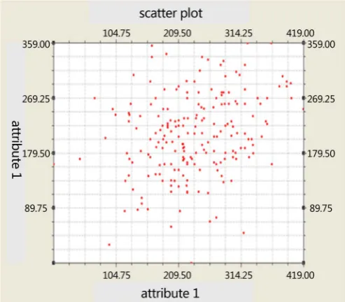
and variance, σ2 respectively. The data in X can be transformed into a new set of data using the simple statistical approach such as the data conversion. The data conversion is applied to the data comparison among attributes, since the parameters and units that represent data group are different, so that they can be compared with each other. That is, xijis converted to yij indicating the degree of distance from the average in (2).
(
.)
.
ij i
ij i
x x
y = σ− (2)
As seen in (2), xi. denote the average of the entity group i. The data of two groups seem to be different before converting data, but it can be proven that those are visually not exact but similar shape after the conversion. And also the minimum value of each attribute is subtracted from all attributes, so that it be-comes a starting point on the X axis and the Y axis respectively after data con-version. As seen in Figure 3, the scatter plot for 2 attributes can be described in two dimensions: attribute 1 on the x-axis and attribute 2 on the y-axis.
In order to classify a lot of points in the scatter plot into many small bundles, the line is drawn with regular intervals as seen in Figure 3. And all entities within a grid are regarded as homogeneous entities. The balanced assignment can be achieved by distributing each entity to subgroups one by one. In this way, the effective balanced assignment can be performed by adjusting the grid spacing.
3.2. MTS Basics
One of the methods on solving a complicate balanced assignment such as an entity having more than 2 attributes is to apply the concepts of the MTS method.
Figure 3. 2 dimensions Scatter plot.
The MTS method is not a new concept but rather a way of combining Dr. Ta-guchi’s concept of quality engineering with the concept of the Mahalanobis dis-tance, a pattern recognition method created by Dr. Mahalanobis. The MTS me-thod should define the Mahalanobis space first. The process of defining the Ma-halanobis space begins with the selection of reference entities and other entities to calculate the Mahalanobis distance. This selection is generally effective in clustering by selecting entities with more or less extreme attribute values rather than selecting entities that are close to the average. This is because, when the da-ta of the attribute has a general and normal distribution, if the entity closer to the average is defined as a Mahalanobis space, the neighboring entities to the average are increased and the clustering effect is halved. Therefore, in this study, the Mahalanobis space is set up as the reference entity with the data having the extreme value among the attributes of the whole entity.
Secondly, in order to obtain the Mahalanobis distance, it requires some ma-thematical processes such as attribute standardization, correlation matrix, and inverse correlation matrix applying (1) and (2). The Mahalanobis distance must be preceded by getting an inverse matrix of covariance using correlation analysis prior to data conversion. However, the correlation matrix can be easily obtained, since the data conversion has already been completed in order to obtain the Mahalanobis distance. The correlation coefficient between attribute i and attribute j is already known as
ij ij
i j
r =σ σσ
× ,
and it becomes σi=1,σj=1 in the standard normal data conversion. As a re-sult, rij =σij and the correlation matrix and the covariance matrix become the
same. Using this inverse correlation matrix, the Mahalanobis distance between
the Mahalanobis space i and entity j is calculated using (1).
3.3. Mahalanobis Space Clustering
The Mahalanobis space is defined as a reference space to measure the Mahala-nobis distance for the purpose of clustering and classification. In general, the Mahalanobis space is a multidimensional space made up of entities of the Ma-halanobis distance smaller than a certain number. Simply the MaMa-halanobis dis-tance is interpreted as a disdis-tance calculation which converts multivariate data into a single numerical value. Since the correlation between attributes is consi-dered, the Mahalanobis distance can be more accurately assessed for the quality of the multi-variate measures compared to the Euclidean distance. If the attributes to be compared are not correlated with each other that means inde-pendent each other, the Mahalanobis distance and the Euclidean distance are almost identical. However, in the analysis of multivariate data with correlation, the accurate distance estimation cannot be done with ignoring this correlation.
For designing purpose of the balanced assignment problem, the definite crite-rion to determine the Mahalanobis space is not specified, and it is determined by the subjective judgment of the designer himself. However, a systematic proce-dure for determining the Mahalanobis space is needed considering the impor-tance of the design depth determined by the designer’s intention, since the op-timal designing conditions determined through the MTS are greatly affected by the Mahalanobis space. Therefore, in this study, we have selected the Mahalano-bis space as the entities with extreme values of each attribute, and applied it to the balanced assignment. In the MTS method, the SNR is used to determine the degree of affecting each attribute by the Mahalanobis space. This is a basic pro-cedure to apply as an evaluation criterion by reducing the low impact characte-ristics and by selecting the high impact charactecharacte-ristics among the various cha-racteristics affecting the Mahalanobis distance.
In this study, the assignment should be made to ensure that the characteristics of the subgroups are similar, and that the attributes included in the characteris-tics are also similar after assignment, assuming that the balanced assignments should be made taking into account all attributes specified in the entity. And all entities in the big group must be distributed and formed the specified number of subgroups. The SNR is obtained to determine the influence between each expe-rimental entity and the Mahalanobis space. The Mahalanobis distance between the Mahalanobis space and the remaining entities is applied as a scale in this study. And the quadratic loss function for the smaller the better is used as seen in (3), since the smaller distance between the Mahalanobis space and the entity means the closer it is.
2 1
1 SNR 10log n ni= yi
= −
∑
(3) The orthogonal array tables are also used to determine which objects are clos-er to the designated Mahalanobis space, before computing the SNR. The size ofthe orthogonal array table is related with the number of entity given. On the or-thogonal array table, 1 means that data is clustered and 0 means that the entity is not used. The fact that the lowest SNR value is selected to the cluster means that the closest entity is clustered. The smaller the SNR, the better it is. And by mul-tiplying negative number, −1 to (3), it can be used as a feature of the higher the better.
4. Experimental Setup
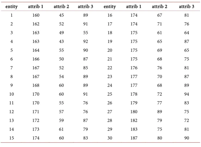
In this section, an example to allocate multiple entities into several subgroups is presented for the validation purpose of the balanced assignment. The example is given by 30 entities and 3 attributes for each entity as shown in Table 1. And the characteristic of subgroup is tried to be similar when all entities are assigned to 3 subgroups.
The result of the MTS method is checked by comparing it against the simula-tion result, and followed by the appropriate analysis.
4.1. MTS Clustering
In order to apply the MTS method, it is necessary to define the Mahalanobis space that can be used as a reference entity. In this study, the entities having the most extreme value of each attribute are set as the reference entities, and those are the Mahalanobis space.
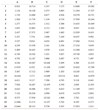
[image:10.595.208.540.488.730.2]Table 2 is shown that 6 entities of A, B, C, D, E, and F are defined as the Ma-halanobis space. In order to compute the MaMa-halanobis distance, the entity by each attribute must be converted using (2), and followed by correlation inverse matrix. The Mahalanobis distance between the Mahalanobis space and each data using (1) is shown in Table 3.
Table 1. 30 entities with 3 attributes.
entity attrib 1 attrib 2 attrib 3 entity attrib 1 attrib 2 attrib 3
1 160 45 89 16 174 67 81
2 162 52 91 17 174 71 76
3 163 49 55 18 175 61 64
4 163 43 92 19 175 65 87
5 164 55 90 20 175 69 65
6 166 50 87 21 175 68 75
7 167 52 85 22 176 76 81
8 167 54 89 23 177 70 87
9 168 60 89 24 177 68 89
10 170 60 91 25 178 72 94
11 170 55 76 26 179 77 83
12 171 57 76 27 180 89 75
13 172 59 87 28 182 79 72
14 173 61 79 29 183 75 81
15 174 60 83 30 187 80 90
Table 2. Mahalanobis space designation.
entity attrib 1 attrib 2 attrib 3 entity attrib 1 attrib 2 attrib 3
A 160 45 89 10 172 59 87
B 163 49 55 11 173 61 79
C 163 43 92 12 174 60 83
D 178 72 94 13 174 67 81
E 180 89 75 14 174 71 76
F 187 80 90 15 175 61 64
1 162 52 91 16 175 65 87
2 164 55 90 17 175 69 65
3 166 50 87 18 175 68 75
4 167 52 85 19 176 76 81
5 167 54 89 20 177 70 87
6 168 60 89 21 177 68 89
7 170 60 91 22 179 77 83
8 170 55 76 23 182 79 72
9 171 57 76 24 183 75 81
Table 3. Mahalanobis distance for given example.
A B C D E F
1 0.923 16.714 5.357 7.175 13.000 19.582
2 1.124 16.120 5.273 5.865 11.364 17.337
3 1.710 13.008 0.677 4.936 19.578 10.751
4 1.926 11.718 1.159 4.710 17.950 10.244
5 1.277 14.575 1.512 3.388 15.655 10.369
6 1.825 15.863 4.712 3.304 9.833 12.452
7 2.437 17.571 2.967 1.682 12.929 8.419
8 5.357 7.754 3.696 7.249 18.937 9.992
9 5.537 8.016 4.016 6.601 17.684 9.214
10 4.239 15.538 2.161 2.356 17.216 5.659
11 5.409 10.435 3.978 4.241 15.308 6.815
12 6.749 14.542 3.321 3.837 19.740 4.855
13 4.792 12.147 5.886 2.607 8.731 7.497
14 6.526 10.567 10.448 5.499 4.500 12.315
15 13.935 6.552 11.220 13.807 22.822 12.700
16 5.567 17.112 3.909 1.203 14.245 4.112
17 10.444 5.171 12.690 10.514 9.661 14.078
18 6.611 9.117 7.596 4.705 9.118 8.441
19 7.926 16.267 12.439 4.330 2.826 11.831
20 6.622 18.496 5.873 0.653 11.189 3.875
21 7.122 20.256 4.990 0.670 14.579 2.892
22 8.575 17.936 10.242 1.868 5.762 6.252
23 12.966 13.172 13.237 5.702 8.530 6.573
24 13.664 20.115 9.738 3.547 17.053 1.511
[image:11.595.206.537.354.727.2]In this study, the SNR is used to compare the influence between each entity and the Mahalanobis space, under the basic condition that all entities corres-ponding to each attribute should be considered and allocated. And finally, the SNR is applied as an indicator to ensure the similarity among subgroups. The quadratic loss function, the smaller the better, is applied as a comparative meas-ure, since the smaller value in the Mahalanobis distance means that the distance between the Mahalanobis space and other entities is close. The orthogonal array table is developed before the SNR is obtained, and L32 orthogonal table is used for the given example.
In the orthogonal array table, each column representing the entities to be as-signed, is used to determine which cluster is closest to the Mahalanobis space. The L32 orthogonal array table is not introduced in this study, since it is given as a basis of the experimental design. By applying (3), the SNR for the designated Mahalanobis space, is presented in Table 4.
The shaded areas in Table 4 represent the most suitable clusters for each Ma-halanobis space. And based on this, the clustered entities is found in the Maha-lanobis space corresponding to the orthogonal array table. The method of as-signing the clustered entities by the Mahalanobis space can be another problem. Here, simply the similarity among subgroups can be guaranteed by distributing the entities belong to the Mahalanobis space in sequential manner. The clustered result by the Mahalanobis space shows that there exists much duplication of ent-ities. The duplicate entities can be regarded as a similar to each other even if they are assigned to any community corresponding to the Mahalanobis spaces. A ba-lanced assignment should be done by assigning the non-duplicated entities first, and then the duplicated entities sequentially.
4.2. Simulation and Comparisons
In this section, the result of simulation is shown by changing the assignment criterion, and comparing it against the result of the MTS method. And the re-sults of other simulations with corresponding to the assigning criteria are shown in Table 5.
As can be seen in Table 5, the results of allocating into 3 subgroups with dif-ferent assigning criteria are examined for the mean and the variance. The as-signment criteria referred in Table 5 arranges the MTS method, random simula-tion, and sequential assignment based on each attribute. The rightmost column in Table 5, the difference means the distance between the maximum value and minimum value after the corresponding assignment. Comparing the result of the MTS method and the simulation results, the results of the MTS method are comparatively satisfactory. And also the correlation between each attribute is examined through simple statistical analysis. The correlation between attribute 1 and attribute 2 is examined to be 0.91, indicating a strong positive correlation. This means that the attributes 1 and attribute 2 can be simplified by combining them into single attribute. The correlations between the other attributes are in-vestigated a negative correlation.
Table 4. Signal to Noise Ratio for given example.
EN SNR (A) SNR (B) SNR (C) SNR (D) SNR (E) SNR (F)
1 −16.993 −23.123 −17.152 −14.784 −23.049 −20.049
2 −14.589 −22.400 −14.499 −15.397 −23.946 −21.010
3 −14.123 −23.404 −16.325 −14.135 −22.273 −21.457
4 −16.564 −24.252 −16.501 −12.740 −22.853 −20.824
5 −15.437 −22.858 −15.939 −14.867 −23.202 −20.656
6 −17.168 −23.332 −17.118 −14.272 −23.352 −20.598
7 −18.497 −22.638 −18.460 −16.466 −23.066 −21.036
8 −16.920 −23.669 −17.760 −15.335 −22.740 −21.028
9 −17.294 −23.752 −17.064 −12.892 −23.040 −19.047
10 −15.034 −21.329 −15.597 −15.714 −23.575 −20.984
11 −16.313 −23.082 −16.923 −15.443 −23.313 −20.638
12 −18.508 −22.932 −18.434 −15.947 −23.000 −20.160
13 −14.672 −23.706 −14.476 −12.748 −23.051 −19.719
14 −17.624 −23.040 −17.962 −14.656 −22.370 −20.141
15 −18.324 −23.455 −17.786 −15.517 −23.162 −20.262
16 −17.172 −23.321 −18.170 −15.539 −22.001 −20.539
17 −16.727 −23.084 −17.788 −14.449 −22.637 −20.261
18 −16.496 −23.433 −16.415 −12.792 −22.901 −19.565
19 −17.950 −22.868 −18.099 −15.960 −22.864 −20.367
20 −17.307 −22.643 −16.879 −15.407 −22.982 −19.786
21 −17.622 −23.601 −16.598 −15.540 −23.551 −19.498
22 −17.516 −22.840 −18.100 −15.397 −22.576 −20.085
23 −16.861 −23.071 −17.546 −14.032 −22.274 −19.614
24 −16.583 −23.460 −16.773 −12.791 −22.793 −19.618
25 −17.447 −22.755 −17.025 −15.235 −23.914 −18.761
26 −18.180 −22.877 −17.162 −16.141 −24.238 −19.017
27 −16.406 −23.268 −17.009 −12.086 −22.625 −18.681
28 −16.563 −22.875 −17.151 −14.050 −22.771 −19.036
29 −17.414 −23.340 −15.426 −14.768 −24.182 −18.363
30 −18.154 −22.241 −18.547 −16.470 −23.452 −20.116
31 −16.041 −23.030 −16.821 −12.063 −22.104 −18.694
32 −16.840 −23.212 −17.545 −13.984 −22.672 −19.805
Table 5. Simulation summary vs. MTS results.
subgroup
criterion attribute
subgroup 1 subgroup 2 subgroup 3 difference
mean variance mean variance mean variance mean variance
MTS
Att1 172.5 49.9 172.7 27.8 172.5 39.1 0.2 22.1
Att2 64.3 34.8 62.2 57.9 63.4 60.4 1.9 25.6
Att3 81.3 44.2 83.4 40.3 81.2 61.9 2.1 21.6
simulation
Att1 172.8 40.3 171.9 50 172.9 47.1 1.0 9.7
Att2 64.5 151.5 61.6 123.4 63.8 112.3 2.9 39.2
Att3 81.6 68.5 83 99.5 81.3 92.2 1.7 31.0
[image:13.595.211.539.590.730.2]Continued
Attribute 1
Att1 172.8 56 172.4 44.5 172.5 41.8 0.4 47.4
Att2 60.9 113.9 63.9 90.5 65.1 191.2 4.2 100.7
Att3 84.8 74.6 81.7 65.6 79.4 121.4 5.4 55.8
Attribute 2
Att1 172.5 42.5 172.1 65.7 173.1 33.7 1.0 32
Att2 64 172.4 63.1 120.5 62.8 112.2 1.2 60.2
Att3 85.2 47.7 86.3 23.3 74.4 110.7 11.9 87.4
Attribute 3
Att1 173.8 43.1 173 44.4 170.9 49.9 2.9 6.8
Att2 66.3 147.8 61.6 109.6 62 133.6 4.7 38.2
Att3 81.5 124.5 82.4 74.7 82 78.2 0.9 49.8
5. Conclusions
In this paper, a balanced assignment methodology is proposed in case of entity with more than 2 attributes. The balanced assignment is a grouping method by matching the mean or variance of the attributes to make each subgroup similar. The Mahalanobis distance is applied to ensure the balanced assignment, and the SNR (Signal to Noise Ratio) is utilized as a measure of classifying large groups with many entities into subgroups. The Mahalanobis distance is a basic idea of the MTS method as a distance indicator considering the correlation of entities in quality control techniques.
Through the simulation, the statistical analyzing process is performed on the balanced assignment by the case study. The results of the MTS method are comparatively satisfied by comparing the result of the MTS method with the si-mulation results. Validations against sisi-mulation data establish the tightness of this approach. By considering that the characteristics of the group before allo-cating are different from those of subgroup after assignment, the basic approach is to try to equalize the mean of each subgroup, and also to try to evaluate the variance representing the quality index of the subgroup.
Finally, for designing purpose of the balanced assignment problem, the stan-dard criterion to determine the Mahalanobis space is not specified, and it is de-termined by the subjective judgment of the designer himself. Therefore, a syste-matic procedure for determining the Mahalanobis space is needed considering the importance of the design depth, since the designation of this space is crucial for finding a better solution.
References
[1] Barron, H. and Schmidt, C. (1988) Sensitivity Analysis of Additive Multi-Attributes Value Models. Operations Research, 36, 122-127.
https://doi.org/10.1287/opre.36.1.122
[2] Dyer, J. and Sarin, R. (1979) Measurable Multi-Attribute Value Functions. Opera-tions Research, 27, 810-820. https://doi.org/10.1287/opre.27.4.810
[3] French, S. (1988) Decision Theory: An Introduction to the Mathematics Rationality.
Ellis Harwood, London.
[4] Taguchi, G., Chowdhury, S. and Wu, Y. (2000) The Mahalanobis-Taguchi System. John Wiley and Sons, Inc.
[5] Taguchi, G. and Jugulum, R. (2002) The Mahalanobis-Taguchi Strategy: A Pattern Technology System. John Wiley and Sons, Inc.
https://doi.org/10.1002/9780470172247
[6] Kim, H. (2010) A Study of Clustering Analysis to Guarantee the Equality of Attributes among Small Group. Master Thesis, Keimyung University, Daegu.