Robird wind tunnel test setup design

(1)

(2)

i

Acknowledgements

After taking courses throughout the first year, the second year of the master program in Systems and Control at the University of Twente (UTwente) is continued with a three month internship and completed with a seven month graduation project. The graduation project I chose is titled “Robird wind tunnel test setup design”. Robird is a robotic bird which establishes flight through flapping. These robotic birds are manufactured by Clear Flight Solutions (CFS). The designed test setup is intended to provide insight in the (aero) dynamics of (Ro) birds, especially in the yet far from fully understood flapping flight, beneficial to both UTwente and CFS. The graduation project is intended for the student to demonstrate his/her ability to independently and creatively integrate the gained knowledge and experience during coursework and the internship while still expanding his/her own knowledge. This has been a process which would not have been possible without the help of others to whom I wish to express my thanks. According to the saying “well begun is half done” I owe Dr. Aarts and Dr. van Dijk my thanks for half the work. Our fruitful discussions on model development in Spacar and controller design enabled me a good kick-off. I thank prof. Hoeijmakers for providing me with insight on the aerodynamic requirements the setup needed to meet. I would like to thank the technicians of the faculty of Engineering Technology (CTW), Norbert Spikker, Theo Pünt, Peter Bolscher, Joop Tiehuis and Martin Spenkeler for their valuable advice on the construction of the test setup and for helping me with manufacturing some of the parts. I would like to thank Freek Tonis of Hankamp Gears for helping me customize the gears I used in the setup. I thank Rob Beltman for helping with the assembly of the setup. I say thanks to Gerben teRietogScholten for the technical advice on the construction of the setup, advice on manufacturers, ordering the parts and for the installation of the controllers and connecting the motors. Again I thank Dr. Aarts. This time for allowing me to work with the force sensor of Mechanical Automation and providing me with the necessary space (in their lab), hardware and software and helping me with the installation and initialization together with Gerald Ebberink and Bert van de Ridder. A thank you goes to Nico Nijenhuis of CFS and his personnel for their advice and enthusiasm. I say thanks to my daily supervisor Ir. Geert Folkertsma for assessing my work critically and not settling for little, allowing me to deliver good quality work. I thank my head supervisor, prof. Stramigioli, for his inspiration and giving me the opportunity and having confidence in me for doing this project. Last but not least, I thank my friends and family for their love and support especially during difficult times.

Thank you! Cyrano Vaseur,

(3)

ii

(4)

iii

Abstract

Robird is a robot bird which mimics flapping motion by two con rod mechanisms per wing which transform motor rotational motion into flapping, i.e. plunging and pitching. The latter caused by introducing a phase shift 𝑝ℎ𝑠 between the motion of the two con rod mechanisms.

To gain understanding in the (aero) dynamics of (Ro) birds, a wind tunnel test setup is designed to among others measure aerodynamic loads. In the design, the desired phase shift 𝑝ℎ𝑠, typically between 6° and 7°, is fixed actively with a desired accuracy of 𝑒𝑚𝑎𝑥= ±0.1°. This is done through the use of two motors (2-DOF). This task is interpreted as a set-point error problem for position control with flapping frequencies 𝑓 up to 7 [Hz].

A nonlinear model of the 2-DOF setup mechanism is developed in Spacar using a finite element formulation. Wing stiffness is modeled as a torsional spring. The model is validated through state space system identification and parameter estimation of the actual setup. Based on an identified simplified linearized model, capturing only low frequency behavior, an optimal PID controller is designed by locating its maximum phase-lead at the desired cross-over frequency dependent on the performance specifications.

However, due to limitations of the applied ELMO controllers cascaded position-velocity (PIP) control is applied instead. The results show that for frequencies up to 𝑓 = 4 [Hz] the desired phase shift (up to 7°) is obtained with the desired accuracy of ±0.1°.

(5)

(6)

v

Summary

Robird is a flying robot bird, currently manufactured in both a peregrine falcon version and a bald eagle version (both birds of prey), which accomplishes flight through a specific flapping wing mechanism. Due to good imitation of its real life counterpart, it can be used in both espionage applications and to scare away birds from places they are undesired at, such as airports and farms.

For a single 2D wing section, bird flapping flight can be described through combined plunging and pitching motion. In Robird, this motion is mimicked by two con rod mechanisms per wing that transform the motor rotational motion into wing flapping, i.e. plunging and pitching. The pitching is caused by introducing a phase shift 𝑝ℎ𝑠 between the motions of the two con rod mechanisms. Although Robird has already achieved flight through flapping, its underlying aerodynamics are far from fully understood. To gain understanding in the (aero) dynamics of (Ro) birds, a wind tunnel test setup must be built. This has been the focus of this graduation project.

The setup to be designed should meet a number of requirements: (i) for freedom in experiments it must allow for an adjustable phase shift 𝑝ℎ𝑠, typically between 6° and 7° with an accuracy of 𝑒𝑚𝑎𝑥= 0.1° for flapping frequencies up to 𝑓 = 7 [Hz], (ii) with it, it must be possible to measure reaction forces and torques in all directions, (iii) for interpretable measurements it must represent a symmetric half of the actual mechanism, (iv) due to wind tunnel dimensions it must be mounted under a quarter turn and (v) to reduce flow disturbances it must be provided with an aerodynamic shield.

For the first requirement, a control and mechanical solution have been combined. In the mechanical solution, the desired phase shift is fixed passively/mechanically through a frictional disc connection. In the control solution on the other hand, the desired phase shift 𝑝ℎ𝑠 is fixed actively through the use of two motors, each predominantly driving a single con rod mechanism. In this way the plant is extended from SISO to TITO. This task is interpreted as a set-point error problem for position control. The position references for both motors are ramp signals with gradients corresponding to 𝑓 = 7 [Hz]. However there is a delay between them, corresponding to the required phase shift 𝑝ℎ𝑠 typically between 6° and 7°. Because both references are controlled individually, the allowed set-point error is set to1₂∙ 𝑒𝑚𝑎𝑥= 0.05°. The chosen control strategy is classic SISO control design combined with decoupling. Regarding the second requirement, a 6-DOF sensor is mounted at the base of the setup and remaining requirements are incorporated into the design straightforwardly. To tackle this position control problem, first a model of the setup mechanism is developed using a finite element formulation using computer software Spacar. The setup mechanism is constructed from elements that are connected through joint nodal and/or deformation coordinates. Hereby the wing stiffness is modeled as a simple torsional spring element. The system coordinates are partitioned in order to describe the system in terms of the degrees of freedom through geometric transfer functions. The system position, velocity and acceleration are described by means of the zeroth, first and first and second order geometric transfer functions respectively. Unlike the velocity and acceleration, the system position cannot be solved analytically due to the highly nonlinear first order geometric transfer function. The position is solved numerically using the Newton-Raphson method and taking into account only the first and second order terms. System dynamics are described by equations of motion which are derived by means of the principle of virtual work and d’Alembert’s principle.

(9)

viii at which this maximum phase-lead appears at the desired cross-over frequency. In such a way, the control parameters are expressed in terms of the desired cross-over frequency. The cross-over frequency on its turn is determined from the maximum allowed set-point error and the chosen reference through the sensitivity function. Also considered is the possible application of plant decoupling prior to SISO control application. The designed controller is tested on the nonlinear model. Hereby rough first estimations (order of magnitude) of the aerodynamic loads are introduced as plant input disturbances. Simulation results showed that the designed controller has been able to deal with these disturbances while still also achieving its target performance. I.e. for a flapping frequency of 𝑓 = 7 [Hz] a phase shift of 𝑝ℎ𝑠 = 7[°] is obtained with an accuracy of 𝑒𝑚𝑎𝑥= ±0.1°

After controller design, mechanical design of the setup is conducted. In addition, a mechanical (passive) solution of the desired phase shift is introduced as an alternative. This is done by means of an optional disc frictional connection established by preload provided through a bolt. Further, the setup is supplied with the needed gears and bearings which have been chosen based on their mechanical sufficiency, i.e. durability against gear tooth side damage and acceptable bearing lifetime respectively. The setup represents a symmetric half of the Robird mechanism, as this was necessary to obtain interpretable aerodynamic loads to be measured. This symmetric half is rotated a quarter turn in order to utilize the wind tunnel dimension optimally with regard to flow disturbances near the walls. Finally, the setup mechanism is provided with an aerodynamic shield to eliminate its flow disturbances as far as possible. This shield is fabricated out of plastic through a vacuum forming process with a designed mold.

Next, setup equipment is selected based on them meeting specific requirements. Maxon motors are chosen based on meeting power, torque, current and electric requirements. Maxon gearboxes are chosen based on meeting transmission and torque requirements. Maxon position encoders are chosen based on meeting resolution requirements. ELMO controllers are chosen based on meeting voltage and current requirements. And a 6-DOF force sensor is chosen based on range and resolution requirements.

After ordering and assembling the parts and equipment, first system identification and parameter estimation is conducted on the plant to gain confidence on the developed model and the controller designed based on it. The stable open-loop (upside-down) plant is sufficiently excited by an appropriate input signal (motor input current). There is chosen for a chirp signal (a sinusoidal signal with increasing frequency) in order to utilize a range of frequencies in one signal. The frequency range is chosen to cover all significant resonances. The signal amplitude is chosen such that the system is excited sufficiently. The sample frequency is restricted by the Nyquist frequency and the highest relevant resonance frequency. System output is measured, and together with the input, first the model order is estimated and next the state space is estimated. The results proved that the developed model fits the experiment. The estimated order (four) was as expected and is in agreement with the theory (model) and the frequency responses showed that the resonances existent in the model are also reflected by the experiment. From the cross-correlation it was found that the model estimation was correct, as this was within the confidence bounds. One obvious difference between the identified plant and the model has been the existence of damping in the actual system and the absence thereof in the model. Hence, damping estimation is conducted and the model is improved with the estimated damping.

(10)

ix caused by e.g. backlash, frictional losses, wrongfully estimated aerodynamic loads or incompleteness of the developed model.

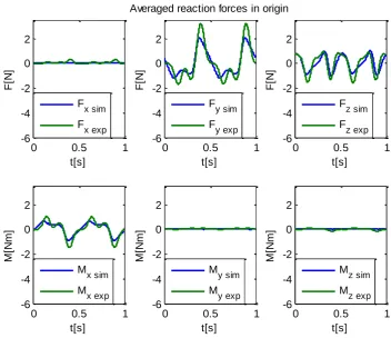
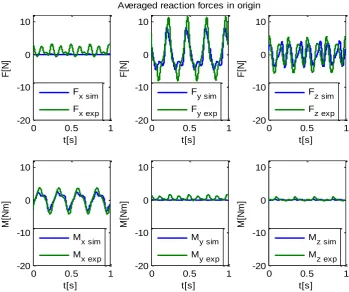
Finally, aerodynamic loads are determined through the measurement of reaction forces with a 6-DOF force sensor. The sensor platform is connected to six 16-DOF load cells through six wire flexures (each rigid in only the longitudinal direction) in an exactly constraint fashion, enabling it to measure forces and torques in all directions. The six load cell voltage measurements are converted to six forces through the load cell sensitivity matrix. Subsequently these forces are, through a conversion matrix, transposed to the reaction forces in the sensor origin. Through a second conversion matrix these forces are transposed to an arbitrary point on the setup. Measurements are compared to simulation results followed by the distinction of aerodynamic loads. The loads are then transposed to the center of the body and alternatively to the center of the wing. Initial reaction force measurements have indicated good agreement with reaction force simulations for low frequencies, i.e. frequencies up to 1[Hz]. For higher frequencies, i.e. above 1[Hz], the measured forces exceed the simulated ones. This is as expected, because the developed model only captures inertia forces and stress resultants whereas the measurements in addition also capture aerodynamic loads. In this way, for wind tunnel experiments to follow, aerodynamic loads can be distinguished by subtracting the measurements from the developed setup with the simulations from the developed model.

(11)

1

1 Introduction

Robird and its application

Robird is a flying robot bird, manufactured by Clear Flight Solutions (CFS) currently in both a peregrine falcon version and a bald eagle version (both birds of prey), which accomplishes flight through a specific flapping wing mechanism.

This robot bird is indistinguishable from its real life counterpart in both looks and motion to both humans and animals. This is exactly why Robird is such an appealing robot. Due to good imitation of its real life counterpart, Robird can be used in both espionage applications and to scare away birds from places they are undesired at, such as airports and farms.

Bird flapping flight

Taking a single two dimensional (2D) wing section, the flapping wing kinematics of a bird are described by two motions occurring simultaneously, namely plunging and pitching, see Appendix 3.1 and for more detail see [1]. This combined motion is determinative for the wing angle of attack which is crucial for achieving flight.

Due to the complex physics behind flapping wing flight in comparison to fixed wing flight, it is far from fully understood and thus leaves room enough for investigation.

Robird’s flapping flight

The Robird flapping wing mechanism is provided with two con rod mechanisms per wing which transform the motor rotational motion into the wing flapping, i.e. plunging and pitching, motion. The latter is obtained by mechanically introducing a phase shift 𝑝ℎ𝑠 into the motion of these two con rod mechanisms.

In such, the flapping wing mechanism on which the flight of Robird is based, requires wing flexibility and causes deformation of the wings, apart from deformation caused by inertial and aerodynamic forces during flapping, and presumably has influences on its flight performance.

Goal

This project is concerned with designing a wind tunnel test setup for the peregrine falcon Robird.

Purpose of the test setup

The designed test setup is intended to provide insight in and understanding of the (aero) dynamics of Robird:

 Body dynamics: Data retrieved from system identification and parameter estimation, using the designed test setup, should serve to improve and validate developed models, e.g. for control design purposes and energy efficiency studies.

(12)

2

Setup requirements

With regard to the purpose of the test setup the following requirements should be met:

1. Adjustable phase shift phs: For freedom in experiments, the test setup should allow for an adjustable phase shift 𝑝ℎ𝑠, typically between 6° and 7°, with an accuracy of 𝑒𝑚𝑎𝑥= 0.1° for flapping frequencies up to 𝑓 = 7 [Hz].

2. Measurement: With the test setup it should be possible to measure reaction forces and torques in all directions.

3. Symmetric half: The setup should represent a symmetric half of the actual mechanism in order to obtain interpretable aerodynamic force measurements.

4. Vertical Orientation: Due to the dimensions of the wind tunnel the setup should be mounted vertically, i.e. under a quarter turn w.r.t. actual mechanism.

5. Aerodynamic Shield: The setup should be provided with an aerodynamic shield to reduce flow disturbances.

Early design choices

 For the first requirement two solutions are considered and combined:

o Control solution: Hereby, in contrast to the actual Robird mechanism, there is aimed at establishing the desired phase shift 𝑝ℎ𝑠 actively through the use of two (servo) motors, each predominantly driving a single con rod mechanism. In this way the plant is extended from SISO to TITO.

This task is interpreted as a set-point error problem for position control. The position references for both motors are ramp signals with gradients corresponding to 𝑓 = 7 [Hz]. However there is a delay in-between them, corresponding to the required phase shift 𝑝ℎ𝑠 typically between 6° and 7°. Because both references are controlled individually, the allowed set-point error is set to1₂∙ 𝑒𝑚𝑎𝑥= 0.05°. The chosen control strategy is classic SISO control design combined with decoupling.

o Mechanical solution: Hereby, optionally the desired phase shift 𝑝ℎ𝑠 is fixed passively/mechanically through a frictional disc connection and consequently both con rods are driven by a single motor.

 With regard to requirement two, a straightforward solution is followed, i.e. a 6-DOF (degrees of freedom) force sensor is mounted at the base of the setup, enabling measurement of reaction forces and torques in all directions.

 The remaining requirements are incorporated in the mechanical design quite straightforwardly.

Approach

(13)

3

2 Model development

First, a model of the proposed TITO setup has been developed in Spacar using a finite element formulation. With the aim at applying position control design, using classic SISO control techniques combined with plant decoupling, the model is linearized and simplified. Referring to the latter, aiming at performance, only the low frequency region is captured for control design.

2.1 Elaborate model development

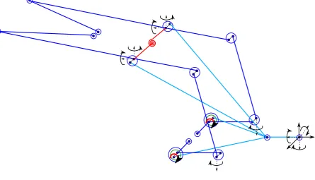
In this section an elaborate non-linear model, also accounting for the coupling of the (servo) motors through the wing stiffness, is developed in Spacar. The developed model contains 2 DOFs accounting for the rotation applied by the motors (see Figure 1).

2.1.1 Kinematic analysis

First all nodal and deformation coordinates of the system are identified. The nodal coordinates 𝑥 are partitioned into support coordinates 𝑥(o), independent nodal coordinates 𝑥(𝑚) and calculable nodal coordinates 𝑥(𝑐), i.e.:

1 𝑥 = [ [𝑥(o)_] [𝑥(𝑐)_] [𝑥(𝑚)_]

]

The deformation coordinates are in turn partitioned into zero deformation coordinates𝜀(o) = 𝐷(𝑥)(o), independent deformation coordinates 𝜀(𝑚)= 𝐷(𝑥)(𝑚) and redundant deformation coordinates 𝜀(𝑐) = 𝐷(𝑥)(𝑐), i.e.:

2 𝜀 = [ [𝜀(o)_] [𝜀(𝑚)_] [𝜀(𝑐)_]

] = [

[𝐷(𝑥)(o)_] [𝐷(𝑥)(𝑚)_] [𝐷(𝑥)(𝑐)_]

]

Then there is checked whether the system is kinematically determinate, simply by evaluating if the number of unknown variables (number of 𝑥(𝑐)) equals the number of useful equations (number of 𝐷(𝑥)(o) and 𝐷(𝑥)(𝑚)).

The number of degrees of freedom within the system equals the number of 𝑥 minus the number of 𝑥(o) minus the number 𝜀(o). For exact restriction, this should be equal to the number of 𝑥(𝑚) and 𝜀(𝑚).

Next, the configuration and deformation state and their derivatives of the mechanism are described in terms of the degrees of freedom which are grouped as follows:

3 𝑞 = [[𝑥(𝑚)] [𝜀(𝑚)_]]

The nodal and deformation coordinates are then described in terms of 𝑞 as follows: 4 𝑥 = 𝐹(𝑞)

(14)

4 These equations, i.e. the zeroth order geometric transfer functions 𝐹(𝑞) and 𝐸(𝑞), are highly nonlinear and the position of the mechanism is solved numerically by use of a Newton-Raphson iteration method. Although the position may not be solved analytically, the velocity and acceleration may be:

After time derivation of Eq.4 and Eq.5, the following applies for the velocities: 6 𝑥̇ = 𝐹_,𝑞𝑞̇

𝜀̇ = 𝐸,𝑞𝑞̇

After time derivation of Eq.6, the following applies for the accelerations: 7 𝑥̈ = 𝐹,𝑞𝑞̈ + (𝐹,𝑞𝑞𝑞̇)𝑞̇

𝜀̇ = 𝐸_,𝑞𝑞̈ + (𝐸_,𝑞𝑞𝑞̇)𝑞̇

Hereby 𝐹,𝑞 and 𝐸,𝑞 are the first order geometric transfer functions and 𝐹,𝑞𝑞 and 𝐸,𝑞𝑞 are de second order geometric transfer functions. In contrast to the zeroth order geometric transfer functions 𝐹(𝑞) and 𝐸(𝑞), these can be solved analytically as will be illustrated in the following. Differentiating Eq. 5 with respect to 𝑞 yields:

8 𝐸_,𝑞= 𝐷_,𝑥𝐹_,𝑞

Rewriting this equation by using the partitioning as introduced in equations1,2 and 3 yields:

9

[ 𝐸,𝑞(𝑜)

𝐸_,𝑞(𝑚) 𝐸_,𝑞(𝑐)]

=

[ 𝐷,𝑥(𝑜)

(𝑜) _𝐷 ,𝑥(𝑐)

(𝑜) _𝐷 ,𝑥(𝑚) (𝑜)

𝐷_,𝑥(𝑚)(𝑜) 𝐷_,𝑥(𝑚)(𝑐) 𝐷_,𝑥(𝑚)(𝑚) 𝐷_,𝑥(𝑐)(𝑜) 𝐷_,𝑥(𝑐)(𝑐) 𝐷_,𝑥(𝑐)(𝑚)][

𝐹,𝑞(𝑜) 𝐹_,𝑞(𝑐) 𝐹_,𝑞(𝑚)]

Then for the first order geometric transfer function applies: 10 𝐹_,𝑞(𝑜) = [𝛿𝑥(𝑜)

𝛿𝑥(𝑚)

𝛿𝑥(𝑜)

𝛿𝜀(𝑚)] 𝐹_,𝑞(𝑚) = [𝛿𝑥(𝑚)

𝛿𝑥(𝑚)

𝛿𝜀(𝑚)] 𝐸_,𝑞(𝑜) = [𝛿𝜀(𝑜)

𝛿𝑥(𝑚)

𝛿𝜀(𝑜) 𝛿𝜀(𝑚)] 𝐸_,𝑞(𝑚) = [𝛿𝜀(𝑚)

𝛿𝑥(𝑚)

𝛿𝜀(𝑚) 𝛿𝜀(𝑚)] 𝐹_,𝑞(𝑐) = (D(𝑐))−1([𝐸,𝑞

(𝑜)

𝐸_,𝑞(𝑚)] − [ 𝐷_,𝑥(𝑜)(𝑚) 𝐷_,𝑥(𝑚)_(𝑚)] 𝐹,𝑞

(𝑚)₎ 𝐸_,𝑞(𝑐) = 𝐷

,𝑥(𝑐) (𝑐) _𝐹

,𝑞(𝑐)+ 𝐷_,𝑥(𝑐)(𝑚)𝐹,𝑞(𝑚) With:

D(𝑐) = [𝐷,𝑥(𝑐) (𝑜)

(15)

5 Differentiating Eq. 8 with respect to 𝑞 yields:

11 𝐸_,𝑞𝑞= (𝐷_,𝑥𝑥𝐹_,𝑞)𝐹_,𝑞+ 𝐷_,𝑥𝐹,𝑞𝑞

Rewriting this equation by using the partitioning as introduced in equations1,2 and 3 yields:

12

[ 𝐸,𝑞𝑞(𝑜)

𝐸_,𝑞𝑞(𝑚) 𝐸_,𝑞𝑞(𝑐)_]

=

[

(𝐷,𝑥𝑥(𝑜)𝐹,𝑞) 𝐹,𝑞 (𝐷_,𝑥𝑥(𝑚)𝐹,𝑞) 𝐹,𝑞

(𝐷,𝑥𝑥(𝑐)𝐹,𝑞) 𝐹,𝑞] +

[ 𝐷,𝑥(𝑜)

(𝑜) _𝐷 ,𝑥(𝑐)

(𝑜) _𝐷 ,𝑥(𝑚) (𝑜)

𝐷_,𝑥(𝑚)_(𝑜) 𝐷_,𝑥(𝑚)_(𝑐) 𝐷_,𝑥(𝑚)_(𝑚) 𝐷_,𝑥(𝑐)_(𝑜) 𝐷_,𝑥(𝑐)_(𝑐) 𝐷_,𝑥(𝑐)_(𝑚)_][

𝐹,𝑞𝑞(𝑜) 𝐹_,𝑞𝑞(𝑐) 𝐹_,𝑞𝑞(𝑚)_]

Then for the second order geometric transfer function applies: 13 𝐹_,𝑞𝑞(𝑜) = [𝛿𝐹,𝑞(𝑜)

𝛿𝑥(𝑚)

𝛿𝐹_,𝑞(𝑜) 𝛿𝜀(𝑚)] 𝐹_,𝑞𝑞(𝑚) = [𝛿𝐹,𝑞(𝑚)

𝛿𝑥(𝑚)

𝛿𝐹_,𝑞(𝑚) 𝛿𝜀(𝑚)] 𝐸_,𝑞𝑞(𝑜) = [𝛿𝐸,𝑞(𝑜)

𝛿𝑥(𝑚)

𝛿𝐸_,𝑞(𝑜) 𝛿𝜀(𝑚)] 𝐸_,𝑞𝑞(𝑚) = [𝛿𝐸,𝑞(𝑚)

𝛿𝑥(𝑚)

𝛿𝐸_,𝑞(𝑚) 𝛿𝜀(𝑚)] 𝐹_,𝑞𝑞(𝑐) = −(D(𝑐)₎−1_[(𝐷,𝑥𝑥

(𝑜)_𝐹 ,𝑞)𝐹,𝑞 (𝐷,𝑥𝑥(𝑚)𝐹,𝑞) 𝐹,𝑞

] 𝐸_,𝑞𝑞(𝑐) = (𝐷_,𝑥𝑥(𝑐)𝐹_,𝑞)𝐹_,𝑞+ 𝐷_,𝑥(𝑐)_(𝑚)𝐹_,𝑞𝑞(𝑐)

Now that the first and second order transfer functions are known, the position can be solved numerically by means of the Newton-Raphson method, hereby taking into account the first and second order terms of the Taylor series expansion of equation 4 and 5:

14 𝑥₍₁₎= 𝑥₀+ (𝐹_,𝑞)₀Δ𝑞 +1

2((𝐹,𝑞𝑞)0Δ𝑞) Δ𝑞 𝜀₍₁₎= 𝜀₀+ (𝐸_,𝑞)

0Δ𝑞 + 1

2((𝐸,𝑞𝑞)0Δ𝑞) Δ𝑞 For more detail on this see [2] and [3].

2.1.2 Dynamic analysis

The dynamics of the system is described by a relatively elaborate equation of motion, which can be derived by means of the principle of virtual work and d’Alembert’s principle (again, for more detail see [2] and [3]):

15 𝑀̅𝑞̈ = 𝐹_,𝑞𝑇_{[𝑓 − ℎ − 𝑀(𝐹}

,𝑞𝑞𝑞̇)𝑞̇] − 𝐸,𝑞𝑇𝜎

Where: 𝑀̅ = 𝐹,𝑞𝑇𝑀𝐹,𝑞 = Reduced mass matrix 𝑀 = Mass matrix

𝑓 = Nodal forces

ℎ = Convective term of the inertia property which is a function of the position coordinates and quadratic in the velocities

𝜎 = Stress resultants calculated from the linear constitutive Kelvin-Voigt equations: 𝜎 = 𝑆𝜀 + 𝑆𝑑𝜀̇ 𝑆 = Stiffness matrix

(16)

6

2.1.3 External forces and reaction forces

Prior to calculating the stress resultants and reaction forces, the motion of the multi-body system must be known already. The external forces (including the reaction forces) can be determined as follows (this is explained very well in [2] and [3]):

16 𝑓 = 𝐷_,𝑥𝑇_{𝜎 + ℎ + 𝑀𝑥̈}

In Appendix 1.1 an example of the kinematic and dynamic analysis as conducted by Spacar is illustrated for a simplified 2D version of the setup mechanism.

2.1.4 Kinematic determinability and exact restriction for the model of the setup mechanism

In the following, kinematic determinability and exact restriction of the developed model for the setup mechanism (see Figure 1) are illustrated.

As discussed in section 2.1.1, the nodal coordinates 𝑥 are partitioned into support/ absolute constraint coordinates 𝑥(o), independent nodal coordinates 𝑥(𝑚) and calculable nodal coordinates 𝑥(𝑐). With their respective numbers 𝑁_𝑥(𝑜), 𝑁_𝑥(𝑚) and 𝑁_𝑥(𝑐) and their sum 𝑁𝑥. The deformation coordinates are

partitioned into zero deformation/ relative constraint coordinates 𝜀(o) = 𝐷(𝑥)(o), independent deformation coordinates 𝜀(𝑚) = 𝐷(𝑥)(𝑚) and redundant deformation coordinates 𝜀(𝑐) = 𝐷(𝑥)(𝑐). With their respective numbers 𝑁_𝜀(𝑜), 𝑁_𝑥(𝑚) and 𝑁_𝜀(𝑐), and their sum 𝑁𝜀.

Kinematic determinability applies if the number of unknown variables matches the number of useful equations, i.e.:

17 𝑁_𝑥(𝑐) = 𝑁_𝜀(𝑜)+ 𝑁_𝜀(𝑚)

Exact restriction applies when the number of user defined DOFs, 𝑁𝑢𝑑𝐷𝑂𝐹, equals the number of resulting DOFs, 𝑁𝐷𝑂𝐹, i.e.:

18 𝑁_𝑥(𝑚)+ 𝑁_𝜀(𝑚)= 𝑁_𝑥− 𝑁_𝑥(𝑜)− 𝑁_𝜀(𝑜)

With:

𝑁_𝑥(𝑚)+ 𝑁_𝜀(𝑚) = 𝑁𝑢𝑑𝐷𝑂𝐹 𝑁𝑥− 𝑁𝑥(𝑜)− 𝑁_𝜀(𝑜)= 𝑁𝐷𝑂𝐹

The following values apply for the numbers of the partitioned coordinates of this system: 𝑁_𝑥 = 120, determined from the sum of:

 (16 × 3) translational coordinates, represented by the (16) blue circles in Figure 1, each representing 3 translational coordinates, 𝑥, 𝑦 and 𝑧 describing a node position

 (24 × 3) rotational coordinates, represented by the (24) blue dots in Figure 1, each representing 3 Euler parameters, 𝜆1, 𝜆2 and 𝜆3 describing a node orientation

(17)

7

 (17 × 6), i.e. 17 fully rigid beams, represented by the (17) blue lines in Figure 1, each restricted in elongation (1 DOF), torsion(1 DOF) and bending (4 DOFs)

 (2 × 2), i.e. 2 partially rigid hinges (restricted in orthogonal bending, 2 DOFs; but free in relative rotation 1 DOF), represented by the (2) green circles in Figure 1

𝑁_𝜀(𝑚)= 2 , i.e. two relative rotations have been chosen as DOFs, see the red arrows in Figure 1. 𝑁_𝑥(𝑚) = 0 , i.e. zero nodal coordinates are chosen as DOFs.

𝑁_𝑥(𝑐) = 108 , i.e. 𝑁_𝑥(𝑐) = 𝑁𝑥− 𝑁𝑥(𝑜)− 𝑁_𝑥(𝑚)

Applying the above determined values to equations 17 and 18 proves the system to be kinematically determinable as well as exactly constraint. I.e., 108 unknown variables (calculable coordinates 𝑁_𝑥(𝑐))

are solved by 108 useful equations (𝑁_𝜀(𝑜) and 𝑁_𝜀(𝑚)) and the 2 user defined DOFs (𝑁𝑢𝑑𝐷𝑂𝐹)

[image:17.595.78.524.268.523.2]

correspond to the 2 resulting degrees of freedom (𝑁𝐷𝑂𝐹).

Figure 1 More elaborate model development in Spacar: Wing stiffness is modeled through a torsional spring (see the red colored element)

2.2 Simplified model illustrating coupling

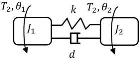
In the following, the elaborate model is somewhat simplified in order to explain the coupling present in the system. The system is reduced to two inertias 𝐽1 and 𝐽2 (each representing half the mechanism) connected to each other by a (rotational) spring 𝑘 and a (rotational) damper 𝑑 (representing the wing) (see Figure 2).

Hence the momentum equation reduces to: 19

𝐽₁𝜃₁̈ = 𝑇₁− 𝑑(𝜃₁̇ − 𝜃₂̇ ) − 𝑘(𝜃₁− 𝜃₂) 𝐽2𝜃2̈ = 𝑇2+ 𝑑(𝜃1̇ − 𝜃2̇ ) + 𝑘(𝜃1− 𝜃2)

(18)

8 20

(𝐽1𝑠2+ 𝑑𝑠 + 𝑘)𝜃1− (𝑑𝑠 − 𝑘)𝜃2 = 𝑇1 −(𝑑𝑠 − 𝑘)𝜃₂ + (𝐽₂𝑠2_{+ 𝑑𝑠 + 𝑘)𝜃}

1 = 𝑇2

In matrix form, this yields: 21 𝐴 [𝜃_𝜃1

2] = [ 𝑇₁ 𝑇2] With:

22 𝐴 = [_𝑎𝑎11 𝑎12 21 𝑎22]

Whereby the following applies for the entries of A: 23

𝑎₁₁= (𝐽₁𝑠2_{+ 𝑑𝑠 + 𝑘)} 𝑎₁₂= −(𝑑𝑠 − 𝑘) 𝑎₂₁= −(𝑑𝑠 − 𝑘) 𝑎₂₂= (𝐽₂𝑠2_{+ 𝑑𝑠 + 𝑘)}

For the transfer function 𝐺 then applies: 24 [𝜃_𝜃1

2] = 𝐺 [ 𝑇1 𝑇₂]

From eqs. 21, 22 and 23 follows for 𝐺:

25 𝐺 = [𝐺_𝐺11 𝐺12 21 𝐺22] = 𝐴

−1_{= [}𝑎11 𝑎12 𝑎₂₁ 𝑎₂₂]

−1

= 1

det(𝐴)[

𝑎22 −𝑎12 −𝑎₂₁ 𝑎₁₁ ]

=_(𝑎 1

11𝑎22−𝑎12𝑎21)[

𝑎22 −𝑎12 −𝑎₂₁ 𝑎₁₁ ]

Substituting eq. 23 into eq.25 and using a preferred notation as described in [4], yields the following for the transfer functions and allows for obtaining physical interpretations of the occurring resonances:

26 𝐺₁₁=𝜃1

𝑇1 =

𝐾( 𝑠2

𝜔𝐴𝑅,12 + 2𝜁𝐴𝑅,1𝑠

𝜔𝐴𝑅,1+1)

𝑠2₍𝑠2 𝜔𝑅2+

2𝜁𝑅𝑠 𝜔𝑅+1)

27 𝐺12=𝜃_𝑇1

2 =

𝐾(𝜏𝑠+1) 𝑠2₍𝑠2

𝜔𝑅2+ 2𝜁𝑅𝑠

𝜔𝑅+1)

28 𝐺₂₁=𝜃2

𝑇1 =

𝐾(𝜏𝑠+1) 𝑠2₍𝑠2

𝜔𝑅2+ 2𝜁𝑅𝑠

𝜔𝑅+1)

(19)

9 29 𝐺₂₂=𝜃2

𝑇2 =

𝐾( 𝑠2

𝜔𝐴𝑅,22 + 2𝜁𝐴𝑅,2𝑠

𝜔𝐴𝑅,2+1)

𝑠2₍𝑠2 𝜔𝑅2+

2𝜁𝑅𝑠 𝜔𝑅+1)

With:

30 𝐾 =_𝐽 1 1+𝐽2

31 𝜏 =𝑑

𝑘

32 𝜔_𝑅 = √𝑘(𝐽1+𝐽2)

𝐽1𝐽2

33 𝜁_𝑅 = 𝑑

2√𝑘𝐽1𝐽2

𝐽1+𝐽2

34 𝜔_𝐴𝑅,1= √_𝐽𝑘 2 35 𝜁𝐴𝑅,1=_2√𝑘𝐽𝑑

2 36 𝜔_𝐴𝑅,2= √_𝐽𝑘

1 37 𝜁𝐴𝑅,2=_2√𝑘𝐽𝑑

1

Hereby 𝜔𝑅 and 𝜁𝑅 represent the resonance/natural frequency and damping of the complete system. 𝜔𝐴𝑅,1 and 𝜁𝐴𝑅,1 represent the anti-resonance and damping equivalent to the natural frequency of inertia 𝐽2 connected to the fixed world through the compliance 𝑘 and damping 𝑑. The equivalent applies for 𝜔𝐴𝑅,2 and 𝜁𝐴𝑅,2.

In this case, due to symmetry of the mechanism, 𝐽1= 𝐽2. Applying this to eqs.32, 34 and 36 yields: 38 𝜔_𝐴𝑅,1= 𝜔_𝐴𝑅,2=1

2√2𝜔𝑅 , for: 𝐽1= 𝐽2, see Figure 4 and Figure 5

Decoupling

Provided there is enough knowledge of the system 𝐺 (through either model development or system identification), one way of decoupling is illustrated in the following. As the goal of decoupling is to obtain a diagonal matrix, the decoupling matrix should bring about the following effect:

39 𝐺𝐷 = [𝐺₀11 _𝐺0 22]

Hence, this would result in a decoupling matrix defined as follows (also see [5]):

(20)

[image:20.595.231.370.93.154.2]

10

Figure 2 Simplified model illustrating mechanical compliant coupling

2.3 Simplified model for controller design

Previous to controller design a sufficient model should be developed. Because performance analysis is a low frequency subject it is acceptable to only model low frequent behavior when analyzing performance (and when designing a controller for performance improvement). The following assumptions are made for obtaining a sufficient model [6]:

 First only 1 DOF is considered (see Figure 3)

 (Half) The wing mechanism is assumed to be a simple rigid equivalent mass (𝑚) to be moved by the actuator force

 The stiffness in the actuated direction is considered to correspond to the low frequency resonance 𝑘 = 𝑚 ∙ (𝜔_{𝑅𝑙𝑜𝑤}2 ) =𝑚∙𝑔_𝐿 ; also see Appendix 6

 The back-emf in the actuator (motor and gearbox) is modeled as damping 𝑑:

41 𝑑 =(𝑘𝑚∙𝑖∙𝜂_𝑅 𝐺)2 With:

𝑘𝑚 = motor torque constant 𝑅 = coil resistance

𝑖 = gear reduction 𝜂_𝐺 = gear efficiency

𝑔 = gravitational acceleration 𝐿 = half length of the wing

 The actuator (motor and gearbox) force is modeled as an applied force:

42 𝐹 =𝑈_𝑅∙ 𝑘𝑚∙ 𝑖 ∙ 𝜂𝐺 = 𝐼 ∙ 𝑘𝑚∙ 𝑖 ∙ 𝜂𝐺 With:

𝑈 = supplied voltage 𝐼 = supplied current

To this end, the following is obtained for the equation of motion: 43 𝑚𝑥̈ = 𝐼 ∙ (𝑘𝑚∙ 𝑖 ∙ 𝜂𝐺) − 𝑘𝑥 − 𝑑𝑥̇

Plant transfer function

Hence with current control (𝑑 = 0; see [6]) the plant model becomes:

𝐽₁ 𝐽2

𝑇₂, 𝜃1 _𝑘 𝑇₂, 𝜃₂

(21)

11 44 𝐺 =𝑥(𝑠)_𝐼(𝑠) = (𝑘𝑚∙𝑖∙𝜂𝐺)𝑚

𝑠2₊𝑑 𝑚𝑠+

𝑘 𝑚

= 1 𝑚𝑒𝑞

𝑘 𝑚

With:

45 𝑚_𝑒𝑞 = 𝑚

𝑘𝑚∙𝑖∙𝜂𝐺

In principle the two actuation directions of the wing mechanism are coupled through the wing stiffness. However at first it is assumed that the system is decoupled, hence it could be easily extended to a 2 DOF i.e. two input two output system as follows:

46 [_𝑥𝑥1 2] =

1 𝑚𝑒𝑞

𝑘 𝑚

[1 0 0 1] [

𝐼1 𝐼₂]

Model parameters

It is worth mentioning that in coming to the values of some of the parameters usage has been made of the more elaborate model developed in which is subject of section 2.1. The values applying to the parameters are given in Table 1.

Bode plot

Supplying all parameters to equation 44 yields the bode plot for 1 DOF of the system as depicted in Figure 5.

Parameter Symbol Value Dimension Reference

Mass (for 1 DOF) 𝑚 0.0441 [kg]

Appendix 1.2 Equivalent mass 𝑚𝑒𝑞 0.0026 [s2⁄_rad2]

Wing stiffness Torsional stiffness 𝑘𝑡 3.35 [Nm rad⁄ ] Appendix 1.3 Longitudinal stiffness 𝑘 1.6 [N m⁄ ]

Motor parameters Torque constant 𝑘𝑚 0.0205 [Nm A ⁄ ]

Chapter 3.4 Coil resistance 𝑅 1.39 [Ω]

Gearbox parameters Gear reduction 𝑖 18 [ ]

Gear efficiency 𝜂𝐺 0.75 [ ]

Table 1 Model parameters

(22)

12

Figure 4 Bode plot for coupled model of Robird

Figure 5 Green: Bode plot for 1 DOF of the simplified model of Robird; Blue: Bode plot for 1 DOF of the coupled model of Robird

-200 0 200 From: Robird/1(1) T o : R o b ir d /1 (1 ) -720 -360 0 T o : R o b ir d /1 (1 ) -200 0 200 T o : R o b ir d /1 (2 )

100 101 102 103

-720 -360 0 T o : R o b ir d /1 (2 ) From: Robird/1(2)

100 101 102 103

Bode Diagram

Frequency (rad/s)

M a g n it u d e ( d B ) ; P h a s e ( d e g ) -100 0 100 200

From: Robird/1(1) To: Robird/1(1)

M a g n it u d e ( d B )

100 101 102 103

-360 -270 -180 -90 0 P h a s e ( d e g ) Bode Diagram

Frequency (rad/s)

with coupling without coupling

𝜔𝑅𝑙𝑜𝑤 𝜔𝐴𝑅 𝜔𝑅

(23)

13

3 Controller and mechanical design

3.1 Control Solution

In this section the control solution is considered whereby the aim is establishing the desired phase shift 𝑝ℎ𝑠 through the use of two (servo) motors. This will require sufficient controller design. The strategy that is followed here is decoupling combined with the application of classic SISO design techniques. The controller is designed based on a simplified model of the system and then tested on the more elaborate model after decoupling. Tests are done first on a linearized model and finally on the non-linear model.

3.1.1 (PID) Controller design

Now, a conceptual PID controller is designed based on the following [6]:

 Proportional control: to set the required cross-over frequency (or bandwidth)

 Integral control: to obtain a small steady state error; i.e. to keep the mass in position when positioning (compensating for the spring force)

 Derivative control: to provide enough phase-margin at cross-over frequency

PID controller

To this end the following conceptual PID controller is obtained [6]: 47 𝐾 =𝑘𝑝(𝑠𝜏_𝑠𝜏𝑧+1)(𝑠𝜏𝑖+1)

𝑖(𝑠𝜏𝑝+1)

Its corresponding frequency plot is shown in Figure 6. As the plot also illustrates the following is indicated by the parameters [6]:

 𝑘𝑝 = Proportional gain

 1

𝜏𝑧 = Corner frequency where derivative action is started

 1

𝜏𝑝= Corner frequency where derivative action stops  _𝜏1

𝑖= Corner frequency where integral action stops Requirements [6]

 The Phase-lag of the integral action should not interfere with phase-lead of the derivative action; i.e. 𝜏𝑖−1 should be lower than 𝜏𝑧−1

 The phase lead of the PID should be used as efficient as possible; i.e. the PID controller parameters are chosen in such a way that the desired cross-over frequency equals the frequency where maximum phase-lead occurs.

PID controller parameters

To this end the PID controller parameters could be expressed in the cross-over frequency [6]: 48

𝜏_𝑧 =√ 1 𝛼

(24)

14 𝜏_𝑝 = 1

𝜔𝑐√1_𝛼

𝑘_𝑝 =𝑚𝑒𝑞𝜔𝑐2

√_𝛼1

𝛼 (the amount of phase-lead) is between 0.1 and 0.3 and 𝛽 > 1. In this case the following is chosen: 49

𝛼 = 0.2 𝛽 = 2

Performance specifications (desired cross-over frequency)

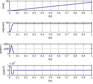
In the previous section the PID controller parameters have been expressed in terms of 𝜔𝑐. It is the focus of the following to determine 𝜔𝑐. The value of 𝜔𝑐 is chosen in such a way that the set-point error (for the constant-velocity part of the reference; this will be explained later) is below 𝑒 = 1₂∙ 𝑒𝑚𝑎𝑥= 0.05° = 8.7 ∙ 10−4_[rad]_{. As}_{𝑒 = 𝑆 ∙ 𝑟}_{, the sensitivity function}_𝑆_{of the system will play an important} role. Also the nature of the reference signal 𝑟 is of great importance.

Bode plot of the PID controller and Block diagram

Figure 6 - Bode plot of the conceptual PID controller [6]

(25)

15

Figure 7 Block diagram of system [6]

Sensitivity function

From the block diagram the following is obtained for the sensitivity function:

50 𝑆 =𝑒

𝑟= (𝐼 + 𝐺𝐾)−1

Low frequent sensitivity function

Applying Eqs. 44, 47 and 48 to Eq. 50 and only considering relevant low frequent behavior (i.e. admissibly disregarding some high order terms; see [6]), the following sensitivity function is obtained [6]:

51 𝑆 =𝑠3+ ( 𝑑

𝑚)𝑠2+ (𝜔𝑛2)𝑠

(𝛼_𝛽)(𝜔𝑐3)

Desired cross-over and servo-error function

From 𝑆 (see eq.50 and eq.51) it follows that the desired 𝜔𝑐 is dependent on the reference velocity, acceleration and jerk; as is the servo error:

52 𝜔_𝑐 = ( 𝑅𝛽𝑘𝑟̇ + 𝑏(𝑘𝑚∙𝑖∙𝜂𝐺)2𝑟̈+𝑅𝛽𝑚𝑟⃛

𝑅𝛼𝑒𝑚 )

1 3

53 𝑒 =𝛽(

𝑘𝑟̇

𝑚 +(𝑘𝑚∙𝑖∙𝜂𝐺) 2_𝑟̈

𝑅𝑚 +𝑟 ⃛ )

𝛼𝜔𝑐3

Equation for reference

The following combination of a 3rd_{order polynomial and linear function, shaping a ramp signal, is taken}

as the reference signal: Eq. 54:

𝑟 =16ℎ𝑚𝑡3

3𝑡𝑚3 , 0 ≤ 𝑡 ≤ (

𝑡𝑚

4)

𝑟 = −32ℎ𝑚( 𝑡3

6−𝑡2𝑡𝑚4 +𝑡𝑡𝑚 2 16−𝑡𝑚

3 192)

𝑡𝑚3 , (

𝑡𝑚

4) < 𝑡 ≤ ( 𝑡𝑚

2) 𝑟 = (2ℎ𝑚

𝑡𝑚) 𝑡 + (−

ℎ𝑚

2) , ( 𝑡𝑚

2) < 𝑡 ≤ ( 𝑡𝑚

2 + ∆𝑡)

Reference signal parameters 𝑡_𝑚 = 0.1[s]

ℎ_𝑚=ω0𝑡𝑚

2 With 𝜔0= 44 [rad_s ]

Plots

Reference signal

(26)

[image:26.595.139.442.99.371.2]

16

Figure 8 Reference signal

Servo-error

Servo error:

Figure 9: Servo error

0 0.1 0.2 0.3 0.4 0.5 0.6 0.7 0.8 0.9 1 0

50

t[s]

r[

ra

d

]

0 0.1 0.2 0.3 0.4 0.5 0.6 0.7 0.8 0.9 1 0

50

t[s]

v

(t

)[

ra

d

/s

]

0 0.1 0.2 0.3 0.4 0.5 0.6 0.7 0.8 0.9 1 0

1000 2000

t[s]

a

[r

a

d

/s

2]

0 0.1 0.2 0.3 0.4 0.5 0.6 0.7 0.8 0.9 1 -1

0 1x 10

5

t[s]

j[

ra

d

/s

3]

0 0.1 0.2 0.3 0.4 0.5 0.6 0.7 0.8 0.9 1 -1

-0.8 -0.6 -0.4 -0.2 0 0.2 0.4 0.6 0.8

1x 10

-3

t[s]

e

[r

a

d

]

(27)

17 The goal set here, is to obtain the performance target as soon as the reference signal reaches the constant velocity part. Hence, the region of interest is the section before the signal changes into the constant velocity part: (𝑡₄𝑚) < 𝑡 ≤ (𝑡₂𝑚), i.e.: 0.025[s] < 𝑡 ≤ 0.050 [s]. Hence, the second line of equation Eq. 54 is substituted into eqs. 52 to obtain the desired cross-over frequency:

𝜔_𝑐 = 126[Hz] = 793[rad/s]

3.1.2 Controller application

In determining the required cross-over frequency, the PID controller has in fact been designed as all its parameters were expressed in 𝜔𝑐 (see equations 47 and 48). In the design of the PID controller, usage has been made of the series form:

47 𝐾 =𝑘𝑝(𝑠𝜏_𝑠𝜏𝑧+1)(𝑠𝜏𝑖+1)

𝑖(𝑠𝜏𝑝+1)

This can be rewritten as follows: 55 𝐾 =𝐾1𝑠2+𝐾2𝑠+𝐾3

𝑠(𝜏𝑠+1)

With: 𝐾1= 𝑘𝑝𝜏𝑧 𝐾₂ =𝑘𝑝(𝜏𝑧+𝜏𝑖)

𝜏𝑖 𝐾3 =𝑘_𝜏𝑝

𝑖 𝜏 = 𝜏_𝑝

Then the series form can be converted to the more usual parallel form of an industrial PID controller (as discusses in [7]) as follows:

56 𝐾 = 𝐾_𝑝+𝐾𝑖

𝑠 + 𝐾𝑑𝑠

𝑠𝜏+1

With:

𝐾𝑝 = 𝐾2− 𝐾3𝜏 𝐾_𝑖 = 𝐾₃

𝐾𝑑 = 𝐾1− 𝐾2𝜏 + 𝐾3𝜏2

With the chosen motor and gearbox the following is obtained for the PID controller parameters: 𝐾𝑝 = 1461

𝐾𝑖 = 2.1559 ∙ 105 𝐾𝑑 = 1.8192

Prior to applying the PID controller to the system, the system is first linearized, decoupled and decoupling matrices are formulated. The PID controller is adjusted with these matrices and thereafter it is applied to the system.

(28)

18 The system is linearized around the working point where both motors have an angular velocity 𝜔0 = 7 [Hz] = 44 [rad

s ] with a desired phase shift 𝑝ℎ𝑠 = 7° = 0.1222[rad] in-between. In Figure 10, the linearized and simplified plant are exhibited.

Decoupling

Due to the wing stiffness, there is quite some coupling in the system. Because applying a PID controller is a SISO control approach, the system first needs to be decoupled (diagonalized). The diagonal PID controller is assisted with input and output matrices such that it experiences the plant as a decoupled one. This is done by the Owens method (see [8]). In applying the Owens method interaction between the modes is removed for a specified frequency regime. Here the chosen regime has been: 0 ≤ 𝜔 ≥ 2𝜔_𝑐. This has been done using the wadyadicd.m script and the decoupling has been successful (see Figure 11).The PID controller is adjusted with the decoupling matrices and has a bode plot as illustrated in Figure 12.

Figure 10 Comparison elaborate and simplified model -200 0 200 From: Robird/1(1) T o : R o b ir d /1 (1 ) -720 -360 0 T o : R o b ir d /1 (1 ) -200 0 200 T o : R o b ir d /1 (2 )

100 101 102 103

-720 -360 0 T o : R o b ir d /1 (2 ) From: Robird/1(2)

100 101 102 103

Comparison elaborate and simplified model

Frequency (rad/s)

(29)

19

Figure 11 Decoupling by means of the Owens method

Figure 12 Adjusted PID controller

100 -600 -400 -200 0 200

M a g n it u d e ( d B ) Bode Diagram

Frequency (rad/s)

100 -600 -400 -200 0 200

Frequency (rad/s)

100 -200 -100 0 100

Frequency (rad/s)

100 -200 -100 0 100

Frequency (rad/s) coupled decoupled -200 -100 0 100 From: In(1) T o : O u t( 1 ) -180 0 180 360 T o : O u t( 1 ) -300 -200 -100 0 100 T o : O u t( 2 ) 105 -90 0 90 180 270 T o : O u t( 2 ) From: In(2) 105 Bode Diagram

Frequency (rad/s)

(30)

20

Control on non-linear plant

(31)

[image:31.842.160.695.87.456.2]

21

(32)

22 The controlled non-linear system gives the following results:

System output:

Figure 14 System output of controlled non-linear system

Servo error:

Figure 15 Servo error of controlled non-linear system

0 0.2 0.4 0.6 0.8 1

-10 0 10 20 30 40 50

t[s]

r[

ra

d

]

Reference1 Reference2 Output1 Output2

0.37 0.371 0.372 15.156

15.158 15.16 15.162 15.164 15.166 15.168

t[s]

r[

ra

d

]

Reference1 Reference2 Output1 Output2

0 0.1 0.2 0.3 0.4 0.5 0.6 0.7 0.8 0.9 1 -2

-1.5 -1 -0.5 0 0.5 1 1.5x 10

-3

t[s]

e

[r

a

d

]

(33)

[image:33.595.106.473.107.389.2]

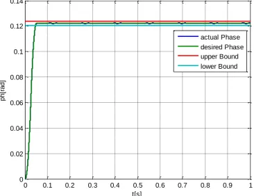
23 Phase shift:

Figure 16 Phase shift of controlled non-linear system

3.2 Mechanical Solution

The main idea here is to mechanically fix the phase shift 𝑝ℎ𝑠 through friction, in particular by using a disc frictional connection. The frictional connection between the discs is established by preload provided by a connection through a bolt. The frictional disc connection ensures that the phase shift is adjustable with an accuracy as high as the measuring equipment allows (see Figure 18)

From the calculations (see Appendix 4) it followed that with a frictional (aluminum) disc connection with a disc radius 𝑟 = 0.015 [m], whereby sufficient preload can be applied by means of a 𝑟𝑏 = 4[mm] radius aluminum bolt (i.e. a M8 – 1.25 bolt), the phase shift can be fixed well to an accuracy as high as the measuring equipment allows. Appendix 4 also illustrates that a spur gear with modulus 1, 36 teeth and a width of 10 [mm] and a radial ball bearing of type 6705 2RS are mechanically sufficient.

Remaining requirements

As Figure 17 illustrates, the setup is oriented vertically, which was required due to the restriction imposed by the wind-tunnel dimensions. The wind tunnel cross-section has a width of 0.9 [m] and a height of 0.7 [m]. Considering the wing with length 0.5 [m] and a flapping angle between 0.6 [rad] and -0.65 [rad] a vertical orientation is more desirable in order to reduce flow disturbance near the walls. As figure 18 illustrates, the setup represents a symmetric half of the actual mechanism in order to obtain interpretable measurements. As is evident in Figure 17 the setup is provided with an aerodynamic shield to reduce flow disturbances. This shield abides by the symmetric requirement. For details on the fabrication of the shield see Appendix 4.4.

0 0.1 0.2 0.3 0.4 0.5 0.6 0.7 0.8 0.9 1

0 0.02 0.04 0.06 0.08 0.1 0.12 0.14

t[s]

p

h

[r

a

d

]

(34)

24

3.3 Comparison and choice

Control Solution

From Figure 16 it followed that for the control solution the phase shift of 𝑝ℎ𝑠 = 7° = 0.1222[rad] is reached with the desired accuracy of𝑒𝑚𝑎𝑥= ±0.1° = ±0.0017[rad]. The drawback of the control solution is that it is less reliable than the mechanical solution.

Mechanical Solution

From the calculations (Appendix 4) it followed that with a frictional (aluminum) disc connection with a disc radius 𝑟 = 0.015 [m], whereby sufficient preload can be applied by means of aM8 – 1.25 bolt aluminum bolt, the phase shift can be fixed well to an accuracy as high as the measuring equipment allows. Although the mechanical solution is more reliable than the control solution, it restricts freedom for experiments significantly. Viz. during operation the phase shift cannot be changed.

Choice

Taking the pros and cons of both solutions in consideration, there is concluded that the most desirable solution is a combination of them both (see Figure 17 and Figure 18). In this way the control solution may be used when more flexibility in doing experiments is required and the mechanical solution may be applied when only a constant phase shift is required or when the control solution fails.

3.4 Equipment selection

The test setup is equipped with two (servo) motors and a 6-DOF force sensor. The placement of this equipment in the Spacar model is indicated in Figure 19 by means of arrows. The two motors are connected in the nodes as indicated by the green arrows and the placement of the force sensor is indicated by the red arrow.

In Figure 20, a complete schematic overview is given for the chosen gearbox, motor, encoder and control unit and the achieved requirements. The selection of these equipment is discussed in Appendix 5 in more detail. In Appendix 5.2.1 and 5.2.2 the selection of an appropriate 6-DOF force sensor and the selection of an appropriate power tool are discussed respectively. In Appendix 8 a brief discussion is given on the working principles of the chosen 6-DOF sensor.

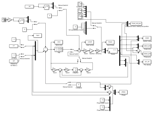
In Figure 22 a schematic overview is given of the applied hardware and software of the complete setup (see Figure 21). Motor Control: Using Elmo controllers with the Composer software, position control is applied on the Maxon motors which are provided with encoders to measure the position. Communication between the Elmo controllers and the Composer software is established through a dual RS232 serial connection using a USB-COM232-PLUS2. Both motors are controlled simultaneously through programs written in the Elmo Studio (see Appendix 7.2). Force measurement: Voltages supplied by the load cells during measurements are first amplified and then, through an NI DAQ platform, are sent and saved to an NI PCI-6221 card on an xPC target computer. With a host computer a DAQ application is developed in Matlab/Simulink and build/downloaded to the target computer via Ethernet connection enabling saving measured data. The measured data is processed and compared to results from the non-linear model developed in Spacar and run in Simulink.

(35)

25

(36)

26

Figure 18 Exploded front view of the setup (without force sensor, wing and aerodynamic shield)

(37)

27

Figure 20 Complete overview of the chosen equipment and the achieved requirement for the control solution

Maxon Planetary Gearhead GP 32 C ∅ 32 𝑚𝑚 (ceramic version):

(𝑖 = 18) → 23 𝜂𝐺 = 0.75

𝑀𝑁,𝐺 = 3 [Nm] >1₂∙ 𝑀𝑚𝑎𝑥 𝑀_𝐻,𝐺 = 3.75 [Nm] > 𝑀_𝑚𝑎𝑥

Maxon EC 32 ∅32, brushless, 80 Watt, CE approved:

𝑀𝑁 = 43.6[mNm] →1₂∙ 𝑀𝑚𝑜𝑡,𝑚𝑎𝑥 𝑀_𝐻 = 355[mNm] > 𝑀𝑚𝑜𝑡,𝑚𝑎𝑥 𝐼𝐻 = 17.3[A] > 𝐼𝑚𝑜𝑡,𝑚𝑎𝑥

∆𝑛

∆𝑀= 6.59 [ rpm mNm] k_n= 465 [rpm

V ] U_max = 24 [V] 𝐼_𝑁 = 2.37[A] →1

2∙ 𝐼𝑚𝑜𝑡,𝑚𝑎𝑥 𝑘_𝑀 = 20.5 [mNm/A] 𝑅 = 1.39 [Ω]

ELMO Whistle 5/60 control unit:

𝑉_𝑐𝑐 = 7.5 – 60 [VDC]

𝑉𝑜𝑢𝑡,𝑚𝑎𝑥 = 0.95 ∙ 𝑉𝑐𝑐 > 0.8 ∙ 𝑉𝑐𝑐 𝐼_max(<1𝑠)= 10 [A] > 𝐼𝑚𝑜𝑡,𝑚𝑎𝑥 𝐼_{𝑐𝑜𝑛𝑡} = 5 [A] >1

2𝐼𝑚𝑜𝑡,𝑚𝑎𝑥

Encoder HED_5540 with 500 CPT:

Transformation: 1

𝑖

Reference signal: 𝑛_{𝑚𝑜𝑡,𝑚𝑎𝑥} = 420[rpm]

𝑒𝑟𝑟𝑜𝑟

(38)

28

Figure 21 Robird wind tunnel test setup

(39)

29

4 System identification and parameter estimation

4.1 Identification plan

Actual open loop (upside down configuration) identification

In this section open loop identification is conducted on the stable upside down configuration (see Appendix 6). The system is excited with an input current and the output angle is measured. Subsequently, state space identification is conducted in Matlab ident. The following current input signal is chosen for system excitation (see the plot of u1 in Figure 23; also see Appendix 6):

 Signal type: In order to capture a number of frequencies in one signal a chirp signal is used for current input.

 Frequency range: Considering the developed model as sufficient guidance (relevant resonances at 𝜔𝑅low = 0.95 [Hz], 𝜔𝐴𝑅,1= 𝜔𝐴𝑅,2= 6.8 [Hz] and 𝜔𝑅 = 9.6 [Hz]) (see Figure

5), a frequency range of 0 [Hz] to 10 [Hz] is chosen.

 Signal amplitude: In order to excite the system sufficient enough while keeping the flapping angle small to neglect aerodynamic forces, an amplitude of 0.2 [A] is chosen.

 Sample frequency: The sample time is restricted by the Nyquist frequency (𝜔𝑁 =𝜔₂𝑠 =_2𝑡1

𝑠) and

the highest relevant frequency (𝜔𝑅), also see Appendix 6: 57 𝜔_𝑁 > 5 ∙ 𝜔_𝑅

For the sample frequency then applies: 58 𝑡_𝑠 < 1

10∙𝜔𝑅

Hence, with 𝜔𝑅= 9.6 [Hz] a chosen sample time of 𝑡𝑠= 0.0072 [s] is sufficient.

Figure 23 system output (position before gearbox; y1 in [counts]) and input u1 (motor current in [A]). Left: Working data and right: Validation data

4.2

Identification results

Order estimation: In ident (Matlab identification tool) a state space model is estimated. From the singular values, first the system order is estimated to be four as expected (see the left side of Figure 24). Frequency response: Next the state space of the system is estimated and the frequency response is plotted. Model residuals: In order to discuss the accuracy of the estimated model the residuals are plotted (see the left plot in Figure 25).

0 5 10 15

-2 0 2x 10

4

y1

Input and output signals

0 5 10 15

-0.5 0 0.5

Time

u1

2 4 6 8 10 12 14

-1 0 1x 10

4

y1

2 4 6 8 10 12 14

-0.5 0 0.5

Time

(40)

30 The fourth order (see Figure 24) estimated system exhibits all three resonances, 𝜔𝑅low, 𝜔𝐴𝑅,1= 𝜔𝐴𝑅,2 and 𝜔𝑅. This is evident in the frequency plot (see Figure 24) and

can also be seen when closely observing the zoomed in working data (see the right part of Figure 25). As the left part of Figure 25 illustrates, i.e. the cross correlation of the input and output data is within the confidence bounds, the estimated model is accurate.

Figure 24 Left: State space order estimation in ident; Right: state space estimated system

Figure 25 Left: model residuals; Right: zoomed in working data

10-2 100 102 104

10-5 100 105

A

m

p

lit

u

d

e

Frequency response

10-2 100 102 104

-200 -100 0

Frequency (rad/s)

P

h

a

s

e

(

d

e

g

)

-20 -10 0 10 20

-1 0 1

Autocorrelation of residuals for output y1

-20 -10 0 10 20

-0.1 0 0.1

Samples

Cross corr for input u1 and output y1 resids

5 10 15

-2000 0 2000

y1

5 10 15

-0.5 0 0.5

Time

(41)

31

5 Model validation and controller redesign

Model validation: Comparison frequency response

Previous to comparing the frequency responses, system damping is measured and added to the Spacar model (see Appendix 6.2). Comparing the frequency response of the estimated system and the modeled system shows that the model fits the measured plant relatively well (see Figure 26). To a great extent, the various resonances agree with each other.

Figure 26 Frequency response of the modeled and estimated system

Controller redesign

Considering the model matches the identified plant well, the controller redesign is considered redundant. I.e. the simplified model based on which the controller has been designed (see equation44) matches the low frequency behavior of the model well.

However, due to limitations of the applied ELMO controllers, application of PID controller did not seem straightforward, instead cascaded position (P) velocity (PI) control is applied. This PIP controller is tweaked using tuning rules as described in Appendix 7.

-100 0 100 200

M

a

g

n

it

u

d

e

(

d

B

)

10-1 100 101 102 103 104

-360 -270 -180 -90 0

P

h

a

s

e

(

d

e

g

)

Bode Diagram

Frequency (rad/s)

(42)

32

6 Controller implementation and tweaking

Due to mechanical limitations of the wing, the controlled system is tested for a flapping frequency up to 4 [Hz], rather than 7 [Hz] that is achieved in-flight. As mentioned previously, due to limitations of the ELMO controllers a tuned PIP controller is implemented instead of the designed PID controller.

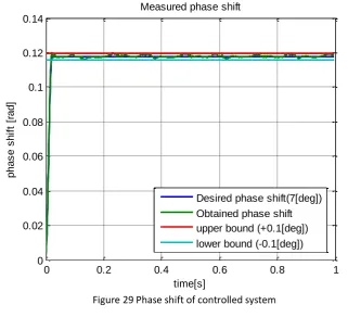
From the results (especially Figure 29) it is clear that for the controlled non-linear system, at a flapping frequency of 4 [Hz], the phase shift of 𝑝ℎ𝑠 = 7° = 0.1222[rad] is reached with an accuracy of 𝑒𝑚𝑎𝑥 = ±0.1° = ±0.0017[rad]. I.e. the target performance of 𝑒𝑚𝑎𝑥= ±0.1° = ±0.0017[rad] is reached.

System output:

Figure 27 System output of controlled system (Right: Zoomed in)

[image:42.595.172.411.500.708.2]

Servo error:

Figure 28 Servo error of controlled system

0 0.5 1 1.5

-5 0 5 10 15 20 25

Reference and measured output

time[s]  [r a d ] _ref1 ₁ _ref2 ₂

0.886 0.888 0.89 0.892 0.894 21.97 21.98 21.99 22 22.01 22.02

Reference and measured output

time[s]  [r a d ] _ref1 ₁ _ref2 ₂

0 0.2 0.4 0.6 0.8 1

-2 -1 0 1 2 3 4 5x 10

-3_{Measured error and allowed bounds}

time[s] p h a s e e rr o r [r a d ] Error

(43)

33 Phase shift:

[image:43.595.127.449.101.393.2]

Figure 29 Phase shift of controlled system

Figure 30 Required motor current

Comparison to simulation

In the following a comparison is conducted between the simulations and experiments of the PIP controlled system. From the error plot of Figure 31 it is clear that, given the same control parameters, even though the measured and simulated current agree rather well in shape (see Figure 32), the measured error is significantly larger than the simulated one. This may be caused by possible occurring loads that are not accounted for in the model.

0 0.2 0.4 0.6 0.8 1

0 0.02 0.04 0.06 0.08 0.1 0.12 0.14

Measured phase shift

time[s]

p

h

a

s

e

s

h

if

t

[r

a

d

]

Desired phase shift(7[deg]) Obtained phase shift upper bound (+0.1[deg]) lower bound (-0.1[deg])

0 0.2 0.4 0.6 0.8 1 1.2 1.4

-10 -5 0 5

Measured motor current

time[s]

I[

A

]

(44)

[image:44.595.110.486.256.555.2]

34

Figure 31 Comparing servo error of the PIP controlled system between simulation and measurements

Figure 32 Comparing required motor current (after detrending) between simulation and measurements

Variable phase shift online

The following figures illustrate that online modification of the desired phase shift is possible very well. However these results do not illustrate complete settling of the response due to limited measurement points provided by the used Composer software, i.e. run time is taken small. In Figure 33 to Figure 36 a varying phase shift 𝑝ℎ𝑠 from 0 [°] to 10 [°] in steps of 2.5 [°] is given for references corresponding to 1 to 4 [Hz] respectively.

0.1 0.2 0.3 0.4 0.5 0.6 0.7 0.8 0.9 1

-5 0 5 10

x 10-3 Comparison simulated and measured error

t[s]

e

[r

a

d

]

error_sim error_meas

0.1 0.2 0.3 0.4 0.5 0.6 0.7 0.8 0.9 1

-4 -3 -2 -1 0 1 2 3 4 5

Comparision simulated and measured current after detrending

t[s]

i[

A

]

Current

motor1,sim

Current_motor2,_sim

Current

motor1,meas

(45)

35

Figure 33 Online phase shift modification: Left: Reference (1 [Hz]); Right: Phase shift

0 0.5 1

0 1 2 3 4 t[s] r[ ra d ] Ref1 Ref2 Out1 Out2

0 0.5 1

-2 0 2 4 6 8 10 t[s] p h [d e g ] phs des phs_act

0 0.5 1

0 2 4 6 8 t[s] r[ ra d ] Ref1 Ref2 Out1 Out2

0 0.5 1

-5 0 5 10 15 t[s] p h [d e g ] phs_des phs_act

0 0.5 1

-2 0 2 4 6 8 10 t[s] r[ ra d ] Ref1 Ref2 Out1 Out2

0 0.5 1

-5 0 5 10 15 t[s] p h [d e g ] phs_des phs_act

0 0.5 1

0 5 10 15 t[s] r[ ra d ] Ref1 Ref2 Out1 Out2

0 0.5 1

Robird wind tunnel test setup design

Acknowledgements

Abstract

Contents

Summary

1

Introduction

2

Model development

2.1

Elaborate model development

2.1.1

Kinematic analysis

2.1.2

Dynamic analysis

2.1.3

External forces and reaction forces

2.1.4

Kinematic determinability and exact restriction for the model of the setup mechanism

2.2

Simplified model illustrating coupling

2.3

Simplified model for controller design

3

Controller and mechanical design

3.1

Control Solution

3.1.1

(PID) Controller design

3.1.2

Controller application

3.2

Mechanical Solution

3.3

Comparison and choice

3.4

Equipment selection

4

System identification and parameter estimation

4.1

Identification plan

4.2

Identification results

5

Model validation and controller redesign

6

Controller implementation and tweaking