Compression rolling of timber: A theoretical model and experimental verification

COMPRESSION ROLLING OF TIMBER A THEORETICAL MODEL

AND EXPERIMENTAL VERIFICATION

A thesis

submitted in fulfilment

of the requirements for the Degree of

Master of Engineering in Mechanical Engineering in the university of Canterbury

By Xixian Deng

CONTENT

ABSTRACT

CHAPTER ONE: INTRODUCTION

1.1 IMPROVEMENT IN THE PROPERTIES OF TIMBER

1.2 THE DEFINITION AND ORIGIN OF COMPRESSION ROLLING 1.3 AIMS AND TASKS OF THE RESEARCH

CHAPTER TWO: LITERATURE REVIEW

2.1 LITERATURE ON COMPRESSION ROLLING PROCESS

2.2 LITERATURE CONCERNED WITH EFFECTS OF COMPRESSION ROLLING OF THE TIMBER BOARDS

CHAPTER THREE: ANALYSIS OF COMPRESSION ROLLING PROCESS

3.1 BASIC ASSUMPTIONS AND INFLUENCE FACTORS OF COMPRESSION ROLLING

3.2 SYMBOLS AND DEFINITIONS

3.3 MATHEMATICAL RELATIONS ON COMPRESSION ROLLING 3.4 THE DYNAMIC PROPERTIES OF COMPRESSION ROLLING OF

TIMBER BOARD

3.4.1 MECHANISM OF BITE AND FRICTION OF COMPRESSION ROLLING PROCESS

3.4.2 THE SPEED OF COMPRESSION ROLLING

CHAPTER FOUR: COMPRESSION ROLLING MACHINE

4.1 GENERAL FUNCTIONS AND FEATURES OF THE COMPRESSION ROLLING DEVICE

4.2 THE FUNCTIONS AND FEATURES OF THE HYDRAULIC POWER SYSTEM

4.3 SPECIFICATION

CHAPTER FIVE: THE APPLICATION OF INSTRUMENTATION AND MICROCOMPUTER FOR MEASUREMENTS AND DATA

ACQUISITION

5.1 THE AIMS AND RANGE OF THE APPLICATION 5.2 MEASUREMENT OF TORQUE AND LOAD

5.2.1 BASIC PRINCIPLE OF THE MEASUREMENT

5.2.2 SIGNAL CONDITIONING CIRCUIT--THE WHEATSTONE BRIDGE FOR STRAIN GAUGES SIGNAL CONDITIONING

5.2.3 RELATED MEASURING DEVICES 5.2.4 CALIBRATION

5.3 MEASUREMENT OF SPEED

5.4 COMPUTER-AIDED EXPERIMENT

5.4.1 THE PRINCIPLE OF ANALOG TO DIGITAL CONVERSION 5.4.2 THE METHODS AND DEVICES INTERFACING TO THE

COMPUTER

5.4.3 COMPUTER PROGRAMME DESIGN FOR THE EXPERIMENT

CHAPTER SIX: EXPERIMENT PROCEDURE 6.1 MATERIAL

6.2 METHODS

6.2.1 DIGITAL IDENTIFICATION SYSTEM 6.2.2 COMPRESSION ROLLING TREATMENTS

6.2.4 MEASUREMENT OF HARDNESS OF TIMBER BOARDS 6.3 METHODS AND PROCEDURE OF DATA PROCESSING

CHAPTER SEVEN: THE RESULTS OF THE EXPERIMENTS

7.1 THE MEASURING RESULTS OF COMPRESSION ROLLING OF TIMBER BOARD

7.2 HARDNESS CHANGE DURING COMPRESSION ROLLING 7.3 RELATIONSHIP BETWEEN MECHANICAL PROPERTIES AND

TREATMENT CONDITIONS

CHAPTER EIGHT: DISCUSSION AND CONCLUSION

8.1 THE EVALUATION AND COMPARISON OF THE RESULTS 8.2 CONCLUSION

8.3 THE PROSPECTIVE RESEARCH FIELDS ON COMPRESSION ROLLING

8.3.1 FROM CLEAR WOOD TO COMMERCIAL GRADE TIMBER BOARD 8.3.2 KNOT EFFECT AND STRENGTH BEHAVIOUR DURING

COMPRESSION

8.3.3 STUDIES ON THE POSSIBILITY OF IMPREGNATING TIMBER USING THE VACUUM OCCURRING DURING THE

DECOMPRESSION PHASE

ACKNOWLEDGEMENT

APPENDIX

APPENDIX 1: PRINCIPLE OF THE RESISTANCE-TYPE STRAIN GAUGE APPENDIX 2: THE SELECTION AND INSTALLATION OF THE STRAIN

GAUGES

A.2.2 SPECIFICATION A.2.3 INSTALLATION

APPENDIX 3: REFERENCE ON HYDRAULIC SYSTEM APPENDIX 4: THE RESULTS OF THE DATA ANALYSIS

ABSTRACT

This research on compression rolling of timber boards concentrates on the following aspects:

1. Analysing the compression rolling process.

2. Developing the instrumentation and the computerized data acquisition to acquire the parameters of

compression rolling.

3. Studying the effects of compression rolling on timber boards

A theoretical model approaches the results of the experiment on compression rolling of timber boards. The surface and properties of timber boards are not obviously changed if the compression level is less than 10%, but are changed to a small degree when the compression level is increased from 10% to 17%%. There are splits and

resin expellation on the surface of timber board when the compression level is more than 17%. The hardness on the surface of the timber boards is increased 4% at 15%

compression level and 6.6% at 17% compression level. This thesis includes eight chapters. Its main contents are Chapter 3 -- theoretical analysis, Chapter 5

application of instruments and the computer, Chapter 6 experiment procedure, Chapter 7

8 -- discussions and conclusions.

CHAPTER ONE:

INTRODUCTION

1.1 IMPROVEMENT IN THE PROPERTIES OF TIMBER

Throughout recorded history, wood has been of enormous economic significance to the development and industrialization of nations. Gradually we have come to recognize that it is very important to improve the

properties of wood and to use it more economically. Many scientists and workers are doing research in this field. This research is concentrated on improving the mechanical properties of wood, such as specific density, hardness, by compression rolling. There are opportunities for using the same technique to aid preservative treatments.

with regard to preservative treatments, numerous methods, biological, chemical and mechanical, have been evaluated. Although many of these processes have had positive results, few have found commercial application. They include solvent seasoning (Ellwood and Ecklund,1963) and other chemical infusions to decrease sap-surface tension (Lantican, Cote, and Skaar,1965), biological pre-treatments (Baueh, Liese, and Berndt, 1970), steaming

Cech,1967).

compression rolling, which has been the subject of a series of investigations over 20 years, is one

mechanical process which offers the prospect of improving wood characteristics.

1.2 THE DEFINITION AND ORIGIN OF COMPRESSION ROLLING The compression rolling of wood is a mechanical and physical process. According to published literature, the process, known as dynamic transverse compression

rolling, originated and was developed in Canada (Goulet 1968). This technique involves feeding sawn timber boards through a pair of contra-rotating rollers. The control parameters of the compression rolling machine are the diameter of the rollers, feed speed and compression level, which depends on the gap between the rollers.

The initial research results using hardwood species (yellow birch) seemed to indicate that a

hydraulic and mechanic combination during rolling induced pit membranes to rupture without causing damage to the cell wall itself. The timber appeared to be opened up for fluid flow, without a significant concomitant loss in mechanical strength (Goulet, Cech and Huffman, 1968; Cech and Huffman, 1970; Cech, 1971). Goulet (1968) claimed savings in the order of 60% in drying of yellow birth after compression rolling. Since Goulet (1968), most research conclusions have been less optimistic.

in drying behaviour. Thus the original claims of Goulet (1968) have yet to be broadly verified.

The research on compression rolling can follow one of two general themes.

1.3 The application of compression rolling to improve of the properties of wood and increase of treatability of timber.

1.4 The study on the theory of compression rolling

The first approach is interested in the effects of compression rolling on physical and mechanical properties and on the treatability of wood, such as drying time and quality, the variance of preservative uptake and

penetration etc •• The second one concentrates on the compression rolling process itself. It seeks to explain the basic changes of wood structure during compression rolling and to explore the reasons for the change in the properties of wood. The latter approach will be used in the project.

1.5 AIMS AND TASKS OF THE RESEARCH

This research is based on a previous project (H. Helge Gunzerodt 1985). The present study is concerned with computerized data acquisition during the

compression rolling process, in an attempt to understand the deformation of wood and the change of physical

The aims and tasks of the research were developed as follows:

1.6 Installation and application of the instrumentation

The dynamometer elements was designed and

installed on the compression rolling machine in order to measure load, torque and speed during compression

rOlling.

1.7 The application of the computer in the experimental process.

A microcomputer and analog-to digital converter were used to guarantee accurate data acquisition and processing.

1.8 The study of the mathematical and mechanical model during compression rolling.

A understanding of the mechanism required a knowledge of the following parameters during rolling:

1.9 Compression level 1.10 Feed speed

1.11 Roller diameter

1.12 Timber characteristics and their interactions with one another.

1.13 Experiments and results

The aim was to establish the factors which

CHAPTER TWO;

LITERATURE REVIEW

2.1 LITERATURE ON COMPRESSION ROLLING PROCESS

There is only a limited literature on the process of rolling of timber and very little attention has been given to the analysis of the compression and

decompression cycle. Previous researches have simply stated that timber boards subjected to such a dynamic loading process behave in a different manner to other materials, such 'as metals or plastics. Although theories concerning the behaviour of these materials during

rolling cannot be directly applied to timber, the

principles developed for other materials are still worth examine.

Wusatowski has described systematically the

principles of compression rolling of metals (Wusatowski 1969, Chapter 3.3).

It assumes that the process of rolling induces strain across the entire cross-section under compression rolling. The stresses in the various cross sections in the area of plastic deformation are different due in part to non uniform speed conditions in the compressed

passing between the rollers. The following simplifying assumptions are made in order to derive slip theories for metal during rolling.

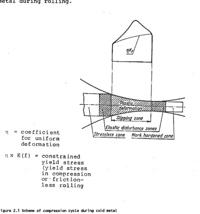
11. = C oe f f i c i en t

for uniform def orma tion

11 x K(f) = constrained yield stress

(yield stress in compression or' friction-less rolling

Elastic disturbance zones

Stressless lone Work hardened zonej

Figure 2.1 Scheme of compression cycle during cold metal rolling (According to Wusatowski, 1969, Pg.208)

1. Plane and perpendicular cross-sections of the initial stock remain also plane and perpendicular after rolling.

[image:12.595.100.509.128.566.2]

3. The coefficient of friction between roll and surface of rolled stock is constant at every point along the

V(r)

=

Peripheral speed of rolls (m/s)

Vip)

=

VCr) x cos 0

veAl

= V-(r) K cos ¢A

V(B)

=

Vir) x cos ¢B

V(Am)= Mean speed of stock in cross section AA V(Bm)= Mean speed of stock in cross section BB

AA,BB= Arbitrarily chosen planes one on each side of the neu tra 1 plane

b = Unit width

2Y (A)

=

Height of rolled stock before 2Y(B)= Height of rolled stock after

ViS) = Volume per second of rolled stock

=

2 x Yep) x cos 0

V(Am) < ViA)

V(Bm) > V(B)

[image:13.595.84.527.137.675.2]

arc of contact.

4. The constrained yield stress is constant along the arc of contact.

5. The rolled material is homogeneous.

6. Rollers are rigid and are not deformed during rolling.

7. stress is acting on each cubic element of any cross section between the rollers.

When analysing the process of compression rolling of timber board, some of these assumptions

above-mentioned may be applied with some modification. In discussing the compression rolling process, Gunzerodt came to the following conclusions:

II The deformation of wood during rolling is very

different to that observed with metals, because of wood's elastic and visco-elastic properties described

previously. Also there is a volume change of the body when rolling wood, which does not occur with metals."

1. Constant volume may not be assumed.

2. Wood does not accelerate through the rollers as it is inextensible to a first approximation in the longitudinal direction and fibres are orientated parallel to the feed direction.

3. The rolled material is inhomogeneous and anisotropic in its three main directions.

4. Elastic deformation is substantially larger than plastic deformation.

5. The constrained yield stress across the thickness of the sample and along the arc of contact varies,

because of the phenomenon of short term surface densification.

6. There are localized density variations in the wood with corresponding fluctuation in MOE, hence the

strain is not uniformly distributed.

Furthermore, one of the main differences in the behaviour of a plastic or ductile material lies in the recovery phase of elasto-plastic materials. Timber must be regarded as a material displaying plastic and elastic characteristics. The proportion of visco-elastic

recovery in the total recovery is a function of the

loading rate. An increase in speed of loading leads not only to higher overall strength values (Kollmann, 1967), but also an increase in the proportion of elastic to visco-elastic recovery (Kollmann, 1961). The effects of

Shain

[ % )

represented in Figure 2.3.

The graph is derived from compression tests perpendicular to the grain of Picea spp. (Kollmann,

Instantaneous

R

e co v e r

y

(i%)

100

, "

" " "

,

.

..

" , , ,

" ·"a.

,

.

,

'

.

,

..

I

f

I

...

-~ _, I

- "f'" I

.. -.,.

..

'"

,

. . . 4o ""

...

".-,

,,'-,

I, ... .

"" "* ... .,..

I

' " , I

;'.,', , , ,

-I ". ,

....

'

.

...

.

... . _... , ~

... .

, ... ~ . "

i

.~

... -...

.

.,.)o---4"'-'-'-''''"''7'-'''''''-t''...,:-:-:---7~'--_'_I_ .... H-+__+_",f60

L

0 ()

d

duration

Figure 2.3 Effects of loading time and compression level on instantaneous recovery of timber compressed perpendicular to the grain (According to Gunzerodt, 1985)

Data for Nothofagus (Gunzerodt): Data for Picea (Kollmann):

Data for Populus (Koch): ..!... • • Extrapolated Data:

1961), Populus tremuloides (Koch, 1964) and Nothofagus fusca (Gunzerodt, 1985).

[image:16.595.48.543.189.545.2]

Figure 2.3 illustrates the relationship between load duration and instantaneous recovery as a function of the compression level. In the course of compression

rolling experiments, the complete loading cycle never exceeds 3 seconds, depending on the feed speed and the roller diameter and would typically be of the order of 0.2 to 0.02 seconds. Typically, after dynamic

compression to 85% of its original thickness the wood will recover to 98.5%. In other words only 10% of the dynamic compression is not recoverable (Cech, 1971). Thus, in the analysis of rolling of wood, Gunzerodt

assumed that creep deformation can be neglected and that the cellwall matrix behaves as a perfect elastic

material.

Previous studies (Gunzerodt, 1985 and Gunzerodt eta at., 1988) on the process of compression rolling of timber indicate that the particular distribution of the total deformation is restricted to the regions in

immediate contact with the surface of the rollers. The concentrated deformation in the upper and lower surface of the timber board can be described as a surface

phenomenon. This has been observed during wood deforming processes under static loading conditions (Kollmann,

1959; Doyle, 1980) and under dynamic loading processes (Johnston and st Laurent, 1978; Peters and Zenk, 1968; Grosditz,1979i Cech, 1972 and Gunzerodt, 1985).

High saturation level reduces the compressibility of the cell voids and fracture occurs in areas of stress concentration (Haslett and Kininmonth, 1975; Gunzerodt, 1985).

On the other hand, when the moisture content of the timber board is below fibre saturation, the cell voids are more compressible and same levels of compression as applied to the highly saturated

samples do not increase the intra-cellular pressure during rolling to the same extent.

2.2 LITERATURE CONCERNED WITH EFFECT OF COMPRESSION ROLLING OF THE TIMBER BOARDS

Compression rolling as a mechanical approach to overcome the resistance of impermeable timbers to

moisture movement, either during drying or during

preservative treatments, was developed in Canada (Goulet, 1968). The process, known as dynamic transverse

compression rolling, had significant influence on the drying characteristics and permeability of species, which had been subjected to the rolling process.

Goulet (1968) supposed that during the compression cycle, damage is induced in the tissue at the microscopic level which has a positive influence on the subsequent drying characteristics and on the treatability of the timber. It was postulated that a combination of

apertures were deformed due to the compression treatment, but no actual evidence of wall failure could be found. Thus, it was believed that opening up the wood structure to fluids during compression rolling does not produce significant concomitant losses in mechanical strength

(Goulet, eech and Huffman, 1968; eech and Huffman, 1970 and eech, 1971).

The previous researches on compression rolling of the timber mainly concentrated on the following two

aspects:

(1). Effect on the drying of timber.

(2). Effect on the treatability of timber.

These studies have been undertaken by a number of workers, but the results vary. In summarizing the

research, the following observations indicate why there are still doubts about the effectiveness and use of compression rolling, despite claims of very sUbstantial improvements in both drying rate and timber quality after drying (Gunzerodt 1985).

1. These studies have been primarily concerned with the drying of hardwood.

2. only hardwoods have been investigated for the

influence of compression rolling on drying in most cases.

4. There are contradictions in the published literature regarding the degree of acceleration in drying even for a single species, such as yellow birch (Goulet 1968, Goulet and Cech 1968, Cech 1971).

5. Disagreement exists regarding the effect of

compression rolling on drying when differing drying schedules are applied (especially concerning the effects of high-temperature schedules).

6. The process proved to be unsuitable for more impermeable timber species such as New Zealand native beeches, Nothofagus fusca and Nothofagus truncata (Haslett and Kininmonth, 1975) partly contradicting an earlier study on drying (eech, 1871), which had indicated that compression rolling could have a more pronounced effect on less

permeable wood.

7. In most of the investigations only limited emphasis was placed on specific asp'ects of machine design and on the various process related parameters, such as feed speed, roller diameter and temperature.

Even though all of the studies on compression rolling of timber are basically concentrated on the effects of compression rolling on both drying rate and treatability, there is some literature dealing with prospect development and profits on compression.

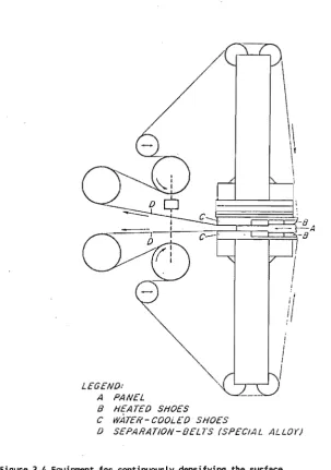
Implication on surface densification of wood: Tarkow and Seborg (1968) undertook research on surface

/1

LEGEND: A PANEL

8 HEATED SHOES

C WATEFr-COOLED SHOES

D SEP.4RATlON-DELl'S (SPECt,.1L ALLOY)

[image:21.595.97.401.258.690.2]

densification of wood in 1968. They used a pair of endless special alloy belts driven by the rollers to press the solid wood panel. Movinq at lineal speeds up to 25 feet per minute, the panel was subjected to a short period of intense heat and pressure and followed by a quick cooling while still under pressure (Figure 2.4).

:...

h.. ~

~ \!J

~ ~

Gj

~ 1.20

1.0.0.

0..80

0..60.

0..40.

REDWo.o.D - SAPWo.o.D.---"" "- _o

0.20.

0..0.0.--o

j_LL--·'---L - - - . l - - - - . J

0.0.4 0.0.8 0..12 0.15

DEPTH FRDM SURFACE (INCHES)

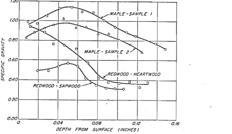
Figure 2.5 Specific gravity gradient of' surface-densified wood

(According to Tarkow and Seborg, 1968)

The experiment results indicated:

[image:22.595.98.496.252.483.2]

from the surface (Figure 2.5)

The abrasion resistance of wood increased at least 15 'times with doubling of the density. The abrasion

resistance of the surface-densified redwood is probably greater than that of normal hard maple.

There are differences between the research on surface densification of wood (Tarkow and Seborg, 1968) and studies on compression rolling of timber (Goulet and eech, 1967; Goulet, 1968; eech and Goulet, 1968; eech, 1971; eech and Pfaff, 1975, etc.), such as, different feed speed (compression rolling with higher speed), different processing temperature (compression rolling with normal temperature, surface densification with high temperature) and different type of compression. Even though there are some differences between the treatments of surface densification of wood and compression rolling, there are surface compression deformation in both case

(Tarkow and Seborg, 1968 and Gu~zerodt, 1985). They might be the cause to produce a certain surface

Tabil.e 2.1 (1) Effects 0f compre's5ion rolling on sawn tilr.ber of' softwood ---~--- ---Botanical Name Common Name Density 3 (kg/m ) Wood maturity Grain or-i en ta tor-ion Moi sture cont. (%)

Abies aiiiaG'Tlis Silver fir Picea graliCa Eastern w.spruce

430 430

lieart-

Heart-wood wood

Not

Flat-consid. sawn

28 - 50 28 - 50

EFFECTS OF COMPRESS ION ROLLING ON Sl>.I'lN TIMBER

Picea CjT"aUCa Eastern w.spruce. 430 Ileart-wood Flat-sawn 38.6

GYNNOSPERHEAE - SOFTWOODS

Picea 9 lauca Eastern w.spruce. 430 Iieart-wood Flat-Sawn 20 pi nus C'Oil'to r t a Lodgepole pine 400 Heart-wood Not consid.

28 - 50

P lnus raffita Rad ia ta pine 400 Sap-wood Flat-sawn Pinus :stro6us Eastern w.pine 380 Heart-wood Flat-sawn

Dry,Redr.1 50 -70

Pseudots. menziesii Douglas fir 500 Heart-wood Not . consid.

28 - 50

Pseudots.

.

.

" menZieSll Douglas fir SOO lieart-wood Flat-quarter

Asuga eteroph. Western Hemlock

---460 --- Heart-Sapwood ---Not consid .

28 - 50 Permea- I Resist.

bility

Resist. I Resist. I Resist. I Resist. I permeablel Mod:rate

I

Resist.

I

Resist. Hod:rate

resist. resist.

Process Creosote (Dr.,Tr.) CCl>. Roller I 152.4 She (mm)

Feed Speed I 253.) (mm/s) Opt. Compr. (

..

) Resul ts and Observa-tions Authors and Da te country

Remarks

10 CCA

up tak e s1 gn if . on faces.

(no edge- penetra-tion) • EW :> LW Satis fac-tory treatment Cooper 1973 Cana da Deta Bed Reference Apparent cor rela-tion: per-meability and den-sity. Influence of intra-specific

Creosote

I

Creosote

I

CCA Creosote

CCA CCA

IS 2.4 I 114.3 I 114. 3 I lS 2 .4

2S).3 I 253.3 I 253.3 I 253.3

10

Creosote up take improved. Face pe-netra tion improved. LN:>EW Inadequat tre atmen t with CCA

Cooper 1973

Canada

Deta iled Rf, poin ts out

problems

i f CL>15% I nd i ca tes role of axial permeabi-lity

15

Increase Pen.58 % Ret,62 % upt. only surfacial

(no edge) sign i f l-cant re ten tion

Cech et

all 1972

Canada

Deta i l ed Reference notes ro-le of un-aspira ted LW pi ts respons i-ble for good LW- permeabi-li ty.

12.5 - I 10

17.5 3.5x

i ncrea se in radial penetra-tion,4.5x in tang. direction Uptake is a sur face phenomena

Cech et

all 1974

Canada

Detailed Reference Indicates

dispro-par tion of CCA.

Increased re ten t ion at lower MC. Problems

Improved creosote face pe-ne tra tion CCA upta-uptake not improved LW > EW

Cooper 1973

Cana da

Deta iled Rf, (see col. 2) Low treatment due to narrow LW layers No expla-na tions of

mechanism

Dry i ng II'l'-Dry ing

?

140.0

10 - 20 Slight reduction in check s when roll ed green.Not eff ec ti ve when dry rolled

Berni et

all 1979

Australia Checking when redry ing trea ted P. radiata cannot be preven tt!d No expla-na tions of mecha-nisms.

?

114.3

2S3.3

8 - 12

Compres-sion surface phenomena leads to stretch-of pit membranes

Grozdits e.a. 1981 Canada

No Data about experim. methods.

Cone 1u-slons based on unpubl. da ta Creosote CCI\. IS 2.4 253.3 10 Improved creosote retention Face pe-netra t ion increased coll apse at CL:>lS% Uptake of

CCl>. not improved Cooper 1973

Canada

Very low uptake only on surface ind ica tes tha t LI>l pr ov ides pa thways. this cau" ses low permcbi-CCA ? ? 15 uptake improved 400 % in fla tsawn boa rds due to damaged pit membranes Nicholas 1973 USA. Conc lu-sion based on unpubli-shed data Very in-comple te

and short

Cr eosote CCA IS 2.4

---,-253.3 --,,---10 CreosO te uptake impro-...ed, subs tan t. on faces. Bigh com-pression

leads to coll apse

Cooper 197 )

Canada

LH:>EW,uni form pe-. netration pattern. De ta i led

~

Tabae 2.1 (2) Effects of c~presaion rolling on sawn timber of hardwood

,,-- ~--

---EFFEc'rs or~ COMP RESS ION ROLL ING ON SAliN TI MBER

---ANGIOSPE~EAE - HARDWOODS

Botanical Name Cammon Name Acer SaCChar. Hard maple Betula all eghan. Yellow birch sp.

Betula papyrif. White bi rch

Euca1yE!.:

obli qU!!

Messmate s tr ingyb.

~£ali:pt.

~gnans

[<Iou n ta in ash

Density 610 640 540 490 700

3 (kg/m )

Wood Heart- Heart- Heart- Heart-

Ifeart-matur i ty ... ·ood wood wood wood wood

Grain or- Flat- Flat- Flat- ? Not

ientation sawn sawn sawn consid.

Nathof a9. lusca Red Beech 530 Heart-wood Flat-sawn Notho! a9. trilncata Hard Beech 600 lieart-wood Not consid. Populus t remuloi. Trembli n9 aspen 450 ? Flat-sawn ~uerclls

r lib r a South. red oak

650

Heart-wood Flat-sawn

~ I---~---;---~---+---_.~

__________ . __________ . __________

+ _ _ _ _ _ _ _ _ _ _ ~ ______

-Moisture con t. (% l

G r e en I G r e en I G r e en G r e en G r e en G r e en G r e en

I

G r e en G c: e en

113.2 110 87.9 85.3 80

Permea-bility

Permeable' M.oder. ~Ioder. Very Very Very ' R e s i s t . ' Resistant' Resist. Resist. Resist. resist. resist. resist.

Process I Drying I Drying I Drying I Drying I Drying I Drying I Drying I Drying I Drying (Dr. I 'I'r. )

Roller I 114.3 I 114.3 I 114.3 '50

? ,

50 150 I 114.3 I 114.3

Size (mm)

Feed Speed' 253.3 (mm/s)

Opt.Campr.1 B - 12

( \ ) Resul ts and Observa-tions Hoderate improve-ment of depth of deforma-tion during rolling

253.3

8.5 -12.5 Possible

to dry at high tempera t. slight reduction . dry i ng

time

253.3

B - 12

Deep dis-tribution of defor-mation in board. Pits da-maged due

to sma 11 size

16.4

10

No improv on drying time nor influence on

shrinkage

? 16.4

? 10

\ -No

impro-vement on drying

S ever e check s in

25\ of boards,no decrease in drying time

16.4

10

Severe checks in 75\ of bds I no de

crease in drying time

253. 3 253.3

8 - 12 7.5

.

_.---.

-No drying

improve-ment.Pit membrane stretched no· spll ts

S light de crease in drying

time I no t

of

economic signific.

---.---4---+---.---~

__________ .. __________ . __________

~

_______

---Grozdits

1

Cech et Author (s)

and Date country

Grozdits

e. a. 1981 USA

Cech 1971 Canada

Grosditz Haslett

1981 e.a. 1975

USA

I

N. Z.

Campbell 1978

Haslett e.a. 1975 Australia' N.Z.

Haslett e.a. 1975 N.Z.

1981 all 1975

---USA Canada

--~-+-.I~-.-+-+-~-

---Remarks Lacks de-tail ed da ta.

I nd i ca tes damage to pits improves drying

through d iftusion

21 % in-crease in

diffusion Evidence

of shear and hy-draulic pressure may

rupture pit mem-branes

Lack s de-ta i led data.pit rupture accounts for high vapor diffusion Conc1us. do not convince

Process not

eft ec tive Machine

not up to s tanda rd

Lacks de-tailed da ta.

~Iain

emphasis on other issues Highly saturated boa rds may explain damage. Machine not adequate Limited emp has is on

rolling due to restrict. machine capacity

SUe tched

p i t mem-branes not con-vincingly interpre-ted.Very

I i mi ted da ta.

Lacks de ta i led da ta. Main emphasis on other

issues

*---_._---CHAPTBR THREB:

ANALYSIS OF COMPRBSSION BOLLING PROCBSS

3.1 BASIC ASSUMPTIONS AND INfLUBNCB FACTORS OF COMPRBSSION ROLLING

Because of its natural origin, the physical properties of timber exhibit a wide degree of

variability. These variations are in part the result of the growth conditions of timber brought about by

environmental factors such as climate, soils, water supply, available nutriments, etc •• In addition, many properties of timber are in part heritable; consequently, a sUbstantial portion of the natural variability of

timber can be attributed to differences in genetic stock. The physical properties of timber are further

complicated by its complex internal structure, which gives rise to anisotropic behaviour. In addition to

natural variability and anisotropy, timber is also porous and inhomogeneous. Because of the inhomogeneity of

timber, there is a wide range of variability in density, strength properties, moisture content, hardness and

In order to simplify the analysis of a compression rolling process, the following basic assumptions have been made:

1. The width of timber boards remains constant during compression rolling.

2. The timber boards are homogeneous and of uniform density and strength properties.

3. Only a small plastic deformation occurs in the timber boards during rolling.

4. The rate of elastic recovery of the timber boards is invariant.

5. The elastic deformation of the timber boards is far greater than plastic deformation during compression rolling.

6. The coefficient of friction between the rollers and the timber boards is constant during compression rolling.

7. Both compression rollers are active rollers and have equal diameter and peripheral speed.

8. The compression rollers are rigid and are not deformed during compression rolling.

3.2 SYMBOLS AND DEFINITIONS

h height of the timber board in any point during rolling.

b width of the timber board

D diameter of the compression roller

hI height of the timber board before compression rolling

h2 minimum height of the timber board during rolling dh absolute compression dimension (dh=h1-h2)

C compression level ( % )

a normal stress L load

E elastic modulus

a bite angle: the angle between the initial contact point and the minimum height point of the timber board

V peripheral speed of the rollers

K a constant which is a factor concerned with modulus of elasticity

H hardness of timber R radius of the roller

t the projection length of AC contact arc on the horizontal plane (refer Figure 3.1)

r the rolling angle

~ shear force P normal force

f1 coefficient of slip friction

e

angle of friction

Pi force on a small area of the contact arc m the feed speed factor

n the hardness factor

f2 coefficient of friction during rolling

z the distance between the centre of the normal force and geometric symmetric centre of the contact arc

3.3 MATHEMATICAL RELATIONS ON COMPRESSION ROLLING Figure 3.1 represents schematically the dynamic

[image:30.595.52.514.192.694.2]

transverse compression rolling process of timber.

According to Figure 3.1, the absolute compression value of timber board is:

where h1 is height of the timber board before compression rolling

h2 is minimum height of the timber board during rolling

thus, relative compression value of timber boards is defined as:

(3.2)

where C is also called compression level

From Figure 3.1, the basic formulae can be derived: (D/2)xcosa

=

D/2-(h1 - h2)/2

and transposing

1-cosa = (h1 - h2)/D

Hence the formula for calculating the angle of bite is found

where

COSa = 1-dh/D (3.3)

a is the angle of bite which is one of the most important factors on compression rolling

D is the diameter of the rollers Furthermore, from Figure 3.1 t 2 = OA2 - OD2

that is, t 2 = R2 - (R-dh/2)2

and neglecting higher-order term

t ~ (dh x R)1/2 (3.5)

From the simplified equation (3.5), the following formula can be deduced,

SINa = t/R ~ (dh x R)1/2/R=(dh/R)1/2 (3.6)

since the maximum bite angle is quite small, in order to simplify the calculation, the sinusoidal value of the bite angle could be replaced by the bite angle itself in radians. For example, in this study, the maximum compression level is 20%, the maximum thickness of the timber board is 33 mm and the diameter of the

rollers is 206.8 mm' thus the maximum bite angle is 14.51 degrees. Obviously, the maximum error caused by the

difference between the sinusoidal value and the radian value of the bite angle is less than 0.03.

Finally, the calculation formula of the bite angle a is deduced as follows:

a

=

(dh/R) 1/2 (rad) (3.7)

From Figure 3.1, the formulae of the rolling angle r and the thickness of the timber board h at any point of contact arc can also be deduced:

COSr = 1-(h-h2)/D (3.8)

3.4 THE DYNAMIC PROPERTIES OF COMPRESSION ROLLING OF TIMBER BOARDS

3.4.1 MECHANISM QF lIT. AND FRICTION IN THE COMPRESSION BOLLING PROCESS

~-+---+--I

I~

I I

~

\1

Figure 3.2 The timber board can not be fed by the rollers (P x SINa > ~ x COSa)

Obviously, at the beginning of compression rolling (that is, when the timber board just contacts the

rollers), the condition of bite is:

P x SINa

=

T x COSa (3.10) The equation 3.10 represents the critical

Figure 3.3 The timber board can be fed by the rollers (P x SINa < ~ x COSa) condition during the feed of the timber boards. where, P is normal force

is shear force

[image:34.595.112.511.241.524.2]

In Figure 3.2, P x SINa is greater than ~ x COSa, thus it is impossible to feed the timber board through the compression rollers; but in Figure 3.3, the timber boards can be fed by the rollers since P x SINa is less than ~ x COSa. According to equation (3.10), we know that the value of P x SINa decreases and the value of~ x COSa increases when the bite angle decreases, that is the possibility of bite increases when the bite angle

decreases, thus we need to find out the maximum bite angle, which can set up the equation (3.10).

It is likely that the maximum angle of bite

depends on the surface condition of the rollers and the timber boards, such as the moisture content of timber boards, the smoothness of the timber boards and rollers, the resin content etc ••

Furthermore, the shear force can be represented:

-r:

= f1 x P (3.11)

where f1 is coefficient of friction

The coefficient of friction can be represented as follows:

f1 = tans (3.12 )

where S is angle of friction

substituting equation (3.11) into equation (3.10) gives: P x SINa

=

f1 x P COSa

hence,

It is known that the coefficient of friction fl is equal to the tangent of the angle of friction, thus,

fl

=

_tanamax

=

tans and then,

(3.I3)

amax =

e

(3.14)

From equation (3.14), the following conclusions can be drawn:

1. The timber boards can be fed by the rollers when the bite angle is less than or equal to the friction angle.

2. The range of the bite angle must be: 0 < a <

e

3. Since the direction change of the resultant normal force, the feed condition is improved when the gap of the rollers is filled by timber boards.

The dynamic friction is caused by slipping between the timber board and the steel rollers at the initial period of feeding. The friction coefficient can be specified within 0.2-0.3 according to previous research results (McMillin etc. 1970, Mckenzie and Karpovich 1968)

3.4.2 THE SPEED OF COMPRESSION ROLLING

The peripheral speed of the compression rollers can be calculated as follows:

where,

D is the diameter of the compression rollers in meters

n is the revolutions per minute of the rollers

Generally, the peripheral speed of the compression rollers represents the feed speed of the timber board. But we must recognize that the horizontal component of the peripheral speed of the compression rollers varies

(Figure 3.4) during compression rolling. For instance, in Figure 3.4, the horizontal component of the peripheral speed of the point A is a minimum VAhl but in the point B, the horizontal component of the peripheral speed is a maximum VBh' Thus, in the arc of the rolling of any point C between A and B, the relationship will be:

(3.16 )

The change of the horizontal component of the

VA

=

V'

COSy

( 0

~

)'"

~

a)

r

Figure 3.5 Sketch of change of the horizontal component on peripheral speed

peripheral speed can be represented schematically in Figure 3.5

From Figure 3.5, we can observe that there is a difference between VAh and VBh " It is the maximum difference of the feed speed, so the maximum relative difference of the feed speed is:

In Figure 3.5, at a certain point, the horizontal component of the peripheral speed can be represented as follows:

where thus,

Vh

=

V x COSr (3.18)

r is the rolling angle (0 ~ r ~ a) (3.19)

VAh

=

V x COSa (3.20)

substituting equations (3.19) and (3.20) into equation (3.17) and simplifying yields,

Vd = (1 - COSa) x 100% (3.21)

To sum up, it is likely that there is a slight slip between the timber boards and compression rollers during rolling.

3.4.3 LOAD AND TORQUE DURING COMPRESSION ROLLING

According to the basic assumptions, we suppose the elastic deformation is far greater than plastic

deformation of the timber boards during compression rolling, thus the timber boards are elastic bodies and Hooke's law can be used.

To simplify the calculations, the following hypothesis is made.

2. The projection length between any two points of the timber board on the horizontal plane is not changed during rolling.

3. The width of the timber board is supposed to be of a unit width.

4. During compression rolling, the relationship of load and normal force, speed and hardness is represented as follows:

(3.22) where,

L is the working load of compression rolling

p _{is the normal force caused by deformation of wood}

V is the feed speed m is feed speed factor

H is the value of wood hardness n is the hardness factor

In equation (3.22), P is the principal parameter which basically determines the range of the load. Item

vm indicates the following fact: The compression rolling

the rollers.

Figure 3.6 describes schematically this phenomenon during the compression rolling process.

In Figure 3.6, all of the compression rolling

Figure 3.6 The effect of the feed speed on the

process of deformation recovery (VI < _V2 < V 3 )

conditions are the same except for the feed speed: VI <

V 2 < V3

the timber boards during compression rolling (such as density of wood, moisture content etc.).

In order to simplify the analysis of compression rolling process and to compare easily the result of the experiments, we take the logarithm of both sides of the equation (3.22), that is,

LnL

=

LnP + m x LnV + n x LnH (3.23)

~:~~~~~~~

~ ~

~~~~rrn~~-r

[image:42.595.125.498.269.669.2]

Furthermore,

P = 1": (Pi) (3.24 )

where, Pi is a force on a small area of the contact arc Figure 3.7 represents schematically the

distribution of the force during compression rolling. From Figure 3.7, we observe that at the point of A,

PA

=

(JA x MA where,

(3.25)

(JA is the normal stress of the timber boards at the point A

MA is the area of the small element

According to the basic principle of the theory of elasticity (Bodig and Jayne, 1982), the normal stress of the timber board can be written as follows:

(J

=

K x Rh (3.26)

where,

K is a constant which is a factor concerned with modulus of elasticity

Rh is compression deformation of timber along the radial direction

Substituting equation (3.26) into equation (3.25) yields, (3.27)

In equation (3.27), the area of the small element MA can be represented ~s follows:

and

(3.29 a) COSr

since the maximum bite angle is quite small and 0

~ r ~ a, in order to simplify the calculation, Rh could be replaced by dh, that is, equation (3.29 a) can be rewritten as follows:

RhA ~ dhA = (hI - h2)/2 - R(1 - COSr) (3.29 b) and the relative error can be indicated:

(3.30) In this research, this relative error is less than 0.03 Substituting equations (3.28) and (3.29 b) into equation

(3.27) and simplifying yield,

PA

=

K x R x (dh/2 - R x (1 - COSr»dr (3.31) PA represents a normal force on a small element which includes the point A of contact arc between the timber board and the roller. In fact, the point A represents any point on the contact arc, so summing up all of the force elements on the contact arc and taking into account the symmetry of the contact arc and the width of the timber board, we get the following equation,

P = 2xbxKxR

r

a

(dh/2 - R x (I-COSr»dr (3.32)

Jo

that is,

where,

b is the width of the timber board

We can further analyse the equation (3.33). Since the maximum bite angle is very small, the sinusoidal

value of the bite angle can be replaced by the bite angle itself in radian, that is,

a ~ SINa

Substituting the above equation into equation (3.33) yields:

P

=

b x K x R x dh x a (3.34 )

Furthermore, substituting equation (3.7) into equation (3.34) and simplifying yields:

P = b x K x ./R x ( dh) 3/ 2 (3.35)

Using the same principle, we can deduce:

where

(3.36)

~ is the resultant shear force caused by friction

1ri is shear force of any small element on the contact arc

During compression rolling of timber boards, the output side portion of the contact arc does not provide the full portion of its normal reaction so that the point at which the centre of normal force is applied always deviates from the geometric centre of the roller. If this distance is z, there is a retarding couple L x Z

following equation can be deduced (Bowden and Tabor, 1963):

T =

=

L x z (3.37a)

Furthermore, comparing equation (3.11), we can get the following equation:

where

(3.37b)

R is the radius of the roller

z is the distance between the centre of the normal force and geometric symmetric centre of the contact arc

T is the compression rolling torque

L is the working load

~ is the resultant shear force caused by resistant friction force

Equation (3.37a) is deduced by considering the following factors:

1. The timber is not perfect. elastic material, so the recovery of compression deformation is a function of time.

2. The contact arc is not geometrically symmetrical during compression rolling (Figure 4 Gunzerodt etc. 1988).

3. The influence of the feed speed and hardness is considered-.

1. First method: the torque based on the resultant shear force

The same principle as equation (3.24), we have,

where

where

~i is shear force on a small area of the contact arc

(3.11a)

Pi is a force on a small area of the contact arc

f2 is friction coefficient during compression Because many factors influence the friction (such as smoothness of the contact surface, moisture content and the condition of the compression rolling), it is very difficult to determine the friction coefficient.

Generally, the friction coefficient during rolling is varied: it is greater than the rolling friction

coefficient and smaller than sliding friction coefficient (Knudson and SChniewind 1971). ' It is likely that this friction coefficient is as a modified rolling friction coefficient. It is caused by two different factors:

(1) slip at the contact arc during rolling. (2) deformation of compression rolling

(Johnson and Tabor 1968)

2. Second method: the torque is based on the retarding couple L X,Z

pattern of the contact arc has already been described in Figure 3.6

We believe the following equation is basically correct with limited experiments:

where

t2 = (1/2 ~ 3/4) x t1

t1 is the projection length of the contact arc on the input side

t2 is the projection length of the contact arc on the output side

The pattern and length of the contact arc and the

If we suppose that: the distance between the

geometrical centre line of the rollers and the centre of the resultant normal force at input side contact arc is 1/3 x t1 and the distance between the geometrical centre line of the rollers and the centre of the resultant

normal force at output side contact arc is 1/3 x t2, then we have the following equation:

T

=

(0.08 - 0.566)t1 x L

-<

Referring to equation (3.35), the normal force P is the function of the width of timber boards, elastic property of timber, the diameter of rollers and

compression level. In the experiments, the item b x K x Rl/2 can be thought of as a single factor and be written as:

p = b x K x Rl/2

Thus, the normal force can be represented as follows: P

=

P

x (dh)3/2 (3.38 a)

We generalize the equation (3.38 a), then we deduce the following formula:

P =

P

x (dh)j (3.38 b)

Equation (3.38 b) is the mathematical generalization formula of equation (3.38 a). substituting equation

(3.38 b) into equation (3.22) yields: (3.39)

Thus, the equation (3.23) can be also represented as: LnL

=

Lnp + j x Ln(dh) + m x LnV + n x LnH (3.40) The equations (3.37a), (3.37b), (3.39) and (3.40) are the basic calculation formulae for analysing compression

CHAPTER FOUR;

THE COMPRESSION ROLLING MACHINE

4.1 GENERAL FUNCTION AND FEATURE OF COMPRESSION ROLLING DEVICE

Figure 4.1 represents schematically the

configuration of the compression rolling device used in this research. This compression rolling machine provides the following functions and features for compression

rolling of timber boards.

1. The machine is easy to operate because the structure of the machine is very simple.

2. The adjustment of the feed speed is reliable, simple and flexible. The hydraulic motors are used to

accomplish speed control with infinite and smooth speed change over a wide range and in either

direction.

3. The design of the machine considers fully a

possibility of installation and usage of measurement instrumentation. with this configuration, the

compression rollers are left unenclosed giving good access to the nip area for observation and

Figure 4.1 The compression rolling device

1. Hydraulic motors

2. Compression rollers

3. The main brackets

4. Load screws 5. Load beams

6. Torque arms 7. The main frame

8. Limited 19ad cylinders

9. The infeed rollers

The compression rolling machine consists of a compression rolling device and a hydraulic power system. Their functions and features are explained as follows:

1. Hydraulic motors: Four low speed and high torque hydraulic motors are used on the compression rolling device. The motors are mounted directly on the ends of the shafts of the compression and infeed rollers. These motors are connected to a variable

displacement pump system. The application of the hydraulic motors provides the following advantages and features:

(A). The hydraulic motors can operate at a low speed that remains constant even when the load

varies.

(B). Infinite and smooth speed control is accomplished easily and economically.

(C). The rotation direction of the motors can be changed instantly with a simple and economic control system. They can rotate continuously and provide equal power output in either direction.

2. Compression rollers: Three pairs of compression rollers are provided. Their diameters are 206.8 mm, 156 rom and 51.8 rom. 206.8 rom diameter compression rollers are called the main compression rollers. The others are the auxiliary compression rollers. The design and installation of the compression

As shown in Figure 4.1, the main compression rollers are installed on the main brackets. The duplex chain is fixed on both sides of the main compression rollers in order to drive other

auxiliary compression rollers at the same peripheral speed as the main rollers.

3. The main brackets: They are used to connect and support the compression rollers and the hydraulic motors. The main brackets are connected and

supported by four long screws rather than a heavy frame. This is one of the features of this

compression rolling device. With this structure, the operators have access to the nip area to measure and observe the compression rolling process at close range.

5. Load beams: On both sides of the two main

compression rollers, there are four load beams, which are used for the installation of the strain gauges and for measuring the load values.

6. Torque arms: As shown in Figure 4.1 and Figure 4.2, there are two torque arms connected to the main brackets and the hydraulic motors. Because of the connection method of the torque arms, they bear pure

D

T

O

, ...

-

--

--

.

---

--.

()

_-~

1 3

torque, thus the torque during the compression rolling of timber board is measured accurately. Each torque arm is connected to each of the

hydraulic motors of the main compression rollers at A and B. At same time, it is attached to each of the main brackets on the side of the hydraulic

motors through simple supports at C and D. A and B are fixed connections carry loads in all three

planes, but C and D are suspended supports and bear torque only. Thus the deformation of the torque arms during compression rolling is the IISIt-shape type deflection (Figure 4.2).

7. The main frame: It connects the other parts of the device and supports the compression rollers and the

infeed rollers.

8. Load hydraulic "cut out" cylinders: They are designed and used for the purpose of safety and protection. The working pressure of the cylinders can be pre-adjusted to supply hydraulic overload protection against large, hard knots in the timber. 9. The infeed rollers: There is a pair of grooved

infeed rollers on the device. Each roller is driven by a hydraulic motor.

10. Infeed rollers adjustment screws: the screws are used f.or adjusting the gap of the infeed

4.2 THE FUNCTIONS AND FEATURES OF HYDRAULIC POWER SYSTEM

The hydraulic power system consists of the

electric motor, the flywheel, the clutch, the VPT 3333 hydrostatic transmission primary unit, the adjustment mechanism (control of displacement of double pump), the filter, the safety valve, the oil reservoir and electric control parts. The principle of the hydraulic system is described schematically in Figure 4.3. The hydrostatic transmission primary unit is composed of two variable displacement hydraulic pumps, check valves, low pressure relief valve, four differential piston type high pressure relief valves and charge pump.

4.3 SPECIFICATION

The power of electric motor

Maximum design compression force Diameter of compression rollers

Diameter of infeed rollers Maximum working width

18 kw 50 KN 51.8 mm 156 nun 206.8 rom

206.8 rom

110 nun Maximum gap between the principal rollers

140 nun

Feed speed 0-3500nun/s

Dimension of the device (nun) 1100x760x1400 Dimension of the hydraulic system (nun)

Figure 4.3 The principle of the hydraulic system 1. Variable displacement hydraulic pumps 2. High torque hydraulic motors

3. The charge pump unit 4. Check valves

5. Relief valves 6. oil tank

7. Pressure gauges

8. Limiting load hydraulic cylinders 9. Throttle valves

.~~

CHAPTER lIVlI

THE APPLICATION OF INSTRUMENTATION AND MICROCOMPUTER FOR MEASUREMENTS AND DATA AggUISITION

5.1 THE AIMS AND RANGE OF THE APPLICATION Figure 5.1 is a diagram, which explains

schematically the principle and range of application of the computer and the instruments.

16 digit input 16 digit out:(.'ut

2 torque arms

Torque signal

I

Strain

UUH

4 lOud be"m.3

trdllsducers

amplifier

I

.. 1

10i,,' d t,';,n::o.:iucf·I·S

n"l sic.:

PCL-712 Multi-Lab Card

- -

- - -

-

- - - - - - - -

-i

16

single-I ended analog

I input ,--~~~~---~~

Overload protected 1;;; bit

I I I I I I I

16 channel WX

SamiJl,~

!ind

hold <:1J, pro:x i mu t i un C(,nvArter I I I I I I I I 1

I 0

1 I I I I

I .

10-I I I I I

I

I I I I I I I

'--Control register Status register

Internal d<J. fa

~ntoro

,... _ _ _ _ _ ..!...:..---, 16 bit

Address decode an d buss

- - - I interface

Counter 1

1 b oj t

Counter 2 1b hit Interrupt _{() __ -=-_~--l}

PC XT Bus

.

.

-5.1

The princ e of application of the computer and the instrum s

I I I

I

I I I I I I I I I .Cutput, ate Out~)ut

Gate I

Clockl

I 21.11 z I I I

5.2. MEASUREMENT OF TORQUE AND LOAD

5.2.1 BASIC PRINCIPLE OF THE MEASUREMENT

The measurement elements of the load and torque--torque arms and load beams have been described in Chapter 4 (Figure 4.2). Each torque arm is part of a torque

dynamometer. Each load beam is one of the elements of a load dynamometer. A torque dynamometer consists of a torque arm, 4 resistance-type strain gauges, direct current power device and the signal amplifier.

Similarly, a load dynamometer is composed of a load arm, 4 strain gauges, DC power device and the signal

amplifier. The position of the torque arms and load

beams and the distribution of the strain gauges are shown in Figure 4.1 and Figure 4.2. A group of four

Since the change of electric resistance is

directly proportional to the change of the strain in the strain gauge and the strain gauges are closely glued to the torque arms or the load beams, the change in the resistance in the strain gauges represents the change in the strain in the torque arms or the load beams, which is caused by torque or load during compression rolling.

Thus, the load of compression rolling represented by the

B

D

II

~;

~

Figure 5.2 Wheatstone bridge circuit on the torque arm

....

'.J

Figure 5.3 Wheatstone bridge circuit on the load beam

:::i

D

II

5.2.2 SIGNAL CONDITIONING CIRCOIT -- THE WHEATSTONE BRIDGE

One of the Wheatstone bridges on the load arms is analyzed as follows. The rest of the Wheatstone bridges have the same principle.

Figure 5.3 represent a Wheatstone bridge on a load beam. The output voltage Eo of the bridge can be

determined by treating the top and bottom parts of the bridge as individual voltage dividers. Thus,

(5.1) (5.2) The output voltage Eo of the bridge is

(5.3)

substituting equations (5.1) and (5.2) into equation (5.3) yields:

(5.4)

Equation (5.4) indicates that the initial output voltage will vanish (Eo

=

0) if

(5.5)

CHANGE OF RESISTANCES IN THE STRAIN GAUGES ON THE TORQUE ARMS OR THE

LOAD BEAMS

CHANGE OF VOLTAGE IN WHEATSTONE BRIDGES MADE UP BY 4 STRAIN GAUGES

ON EACH OF TORQUE ARMS OR LOAD BEAMS

CHANGE OF THE STRAINS IN THE STRAIN GAUGES

CHANGE OF THE STRAINS IN EACH OF THE TORQUE ARMS OR LOAD BEAMS

THE LOAD OF EACH LOAD BEAM OR THE TORQUE OF EACH TORQUE ARMS

TORQUE OR LOAD OF COMPRESSION ROLLING

(R1+dR1)x(R3+dR3)-(R2+dR2)x(R4+dR4)

dE o=Eix---(5.6) (Rl+dRl+R2+dR2) x (R3+dR3+R4+dR4)

Expanding, neglectihg higher-order terms and substituting equation (5.5) yields:

Rl dRl dR2 dR3 dR4

dEo=---x(----

-

---- +

----

-

----)xEi

(Rl+R2) 2 Rl R2 R3 R4

Equation (5.7) indicates that the output voltage from the bridge is a linear function of the resistance changes. This apparent linear results from the fact that higher-order terms in equation (5.6) are neglected. If the higher-order terms are retained, the output voltage dEo

is a nonlinear function. since the resistances of each of the strain gauges on the load beam are same, the equation (5.7) can be deduced:

since the distribution of the strain gauges on the load beam is symmetrical, the strains on gauge 1 and gauge 3 are the same and the strains on gauge 2 and gauge 4 are also the same, that is,

where _{dRc is the change of resistance in gauge 1 or} gauge 3 due to uniaxial compression.

dRt is the change of resistance in gauge 2 or gauge 4 caused by uniaxial tension. According to symmetry, from equation (5.8) the

following equation is deduced:

IdEOI={2xldRc l+2x/ dRtl)/4XR (5.9) then,

IdEol = dR/R (5.10)

By neglecting the installation error of the strain gauges and the error caused by the strain gauges

performances, the strain of the load beam can be deduced from Appendix 1, that is:

& = l/GF x dR/R (5.11)

To sum up: the resistance change of the strain gauges of the load beam is converted into the change of voltage by the Wheatstone bridge and this change

calibration, we can set up a relationship between the load and the voltage of the Wheatstone bridge.

For the principle of the resistance-type strain gauges also refer to Appendix 1. For the selection and installation of the strain gauges refer to Appendix 2 in detail.

5.2.3 RELATED MEASURING DEVICE

The following devices are used for the measurement of load and torque.

(1). The strain gauge amplifier. (2). DC power device

(3). Terminal Block

(4). PCL-712 Multi-Lab Card (5). PC XT

(6). PCLD-780 wiring terminal board

The principle and application of these devices will be described separately.

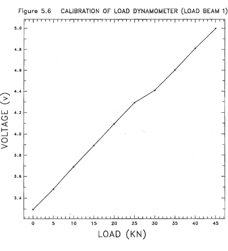
5.2.4 CALIBRATION

voltage can be deduced by data processing.

The calibration procedure of each of the two load dynamometers was described as follows:

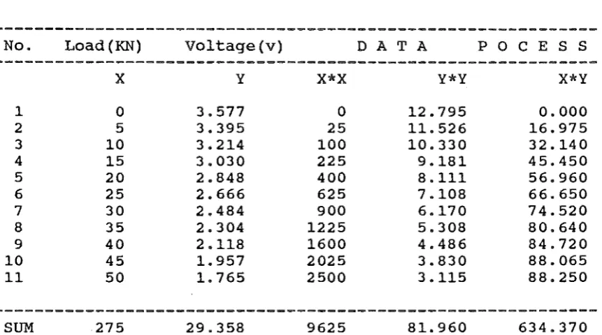
(1). First of all, a load cell must be calibrated. It is connected with the strain gauge indicator in the full Wheatstone bridge and loaded up by means of uniaxial compression on the universal testing

machine from 0 KN to 50 KN at interval of 5 KN. The readings of the strain values from the strain gauge indicator are recorded. These readings correspond to each load.

(2). Secondly, the load cell is placed between the two compression rollers. Both top and bottom

(3). The load cell is placed under load by closing the gap between two compression rollers. A hand pump is connected to the two "limit load" cylinders at the bottom of the two long screws (Figure 4.1) and need to pump the hydraulic oil into the

--- ~

~I

Figure 5.5 Calibration of the load dynamometers Legend: 1, 2

3, 4 5

The compression rollers Aluminium Blocks

Load cell and measurement system

cylinders. The two cylinders push the bottom compression roller upwards and so place the load cell under load. The voltage values of each of load dynamometers are recorded when the load is

(4). The results of data processing and the load-voltage curve are shown in Table 5.1, Table 5.2, Figure 5.6 and Figure 5.7.

1

I