Linear location estimators : the dependence of their quality on the shape of the probability density function, and their robustness

(1)

LINEAR LOCATION ESTIMATORS: THE DEPENDENCE OF THEIR QUALITY ON THE SHAPE OF THE

PROBABILITY DENSITY FUNCTION, AND THEIR ROBUSTNESS.

A thesis

submitted for the degree

of

Doctor of Philosophy in Mathematics

in the

University of Canterbury

by

Peter M. Heffernan

University of Canterbury Christchurch, New Zealand

(2)

for: "Linear Location Estimators: the Dependence of their Quality on the Shape of the Probability Density Function, and their Robustness by Peter M. Heffernan

University of Canterbury, Christchurch, New Zealand: 1980. p16 , line

2-pl7 , line 6

p45 , line 3

''at± K." should be. "at± K (assu.Il}i~g J.t=O) ."

"+

I:

II should be

"+

2

I: "

II ( 5 I 8) 1 ( 8 I 8) and ( 8 1 9) II II ( 4 1 8 ) 1 ( 7 I 8) and ( 7 1 9 ) II

should be

p51 , Table 3.2.2, entry at (1.5,0.16)

"5.496 & 95.071"

should be "95.496 & 95.071"

p59 , Table 3.2.10, entry at

(1.625,0.055)

".499 & 97.584"

should be "97.449 & 97.584"

p67 , line 2

p94 , line 4

p97 , line 9

"good-of-fit11 _{should be} _{"goodness-of-fit"}

"variance c11

II 1 II

n should be

should be "covariance c"

II 1 II n2

pl05, lines 7 and 8 "Except for the first two distributions" should be

"Except for the first two distributions and the last distribution"

plll, line 2· "receiving positive weight" should be "receiving significant positive weight"

pl29, line 2 11 f011

(3)

PHYSICAL SCIENCES LIBRARY

CONTENTS

CHAPTER PAGE

ABSTRACT . . • . . . , . . . • . . . 1

ACKNOWLEDGEMENTS . • . . . • . . . • 2

1 INTRODUCTION I fl "!. 9 6 ~ • • Ito . . . t • 1 • .f • lf • 3

2 THE DEPENDENCE OF THE BEST LINEAR ESTIMATOR ON 'rHE SHAPE OF THE DENSITY FUNCTION FOR NEAR-NORMAL

DISTRIBUTIONS 7

2.1 Introduction . 7

2.2 The Measure of Quality of an Estimator . . 8

2.3 The Organization of the Distributions 12

2.4

2.5

2.6

The Estimators .

The Calculations

Analysis of the Results for N

=

8

21

. . . 21

27

3 THE ROBUSTNESS OF LINEAR ESTIMATORS ON NEAR-NORMAL DENSITIES OF VARIOUS SHAPES

3.1 Introduction .

3.2 Robustness of Efficiency .

. 46

46

47

3.3 Robustness on Distributions with Variance

One • • • 62

3.4 Robustness on Scaled Distributions . . . . 68

(4)

4 FEATURES OF PROBABILITY DENSITY FUNCTIONS WHICH

APPENDIX

INFLUENCE THE FORM OF GOOD ESTIMATORS . 4.1 Introduction . . • . . . 4.2 The Best Linear Estimators for Step

• • • 88

• • • 8 8

Distributions • • • • • 9 0

4.3 The Effect of Features of the Density Function on Estimation for Other

4.4

Distributions . Conclusion REFERENCES

. . 116 . . 123 128

1 THE NEAR-NORMAL DISTRIBUTIONS . . . 130

2 THE COEFFICIENTS AND VARIANCES OF THE BEST LINEAR LOCATION ESTIMATORS FOR THE NEAR-NORMAL

DISTRIBUTIONS FOR SAMPLE SIZES OF 4, 8 and 16 . . 155

3 THE EXPECTED VALUES OF THE ORDER STATISTICS FOR SAMPLES OF SIZE 4, 8 AND 16 FROM THE NEAR-NORMAL DISTRIBUTIONS . • • • • • . • • • • • 17 2

4 THE COVARIANCES OF THE ORDER STATISTICS FOR

(5)

APPENDIX PAGE 5 THE PERFORMANCE OF VARIOUS ESTIMATORS ON THE

6

SET OF NEAR-NORMAL DISTRIBUTIONS,AND THE FAC~ORS

BY WHICH THESE DISTRIBUTIONS ARE SCALED IN ORDER TO STANDARDIZE THEIR 95TH PERCENTILES .

THE STEP DISTRIBUTIONS

• 204

. 220

7 THE COEFFICIENTS AND VARIANCES OF THE BEST LINEAR LOCATION ESTIMATORS FOR THE STEP DISTRIBUTIONS

FOR SAMPLE SIZES OF 4, 8, 16 AND 32 . . . 224

8 THE EXPECTED VALUES OF THE ORDER STATISTICS FOR SAMPLES OF SIZE 4, 8, 16 AND 32 FROM THE STEP DISTRIBUTIONS .

9 THE COVARIANCES OF THE ORDER STATISTICS FOR SAMPLES OF SIZE 4, 8, 16 AND 32 FROM THE STEP DISTRIBUTIONS . . . • •

10 THE COMPUTER PROGRAM FOR CALCULATING THE BEST LINEAR ESTIMATORS FOR THE NEAR-NORMAL

. . 231

. . 236

(6)

ABSTRACT

The dependence of the performance of linear location estimators on the shape of the probability density function is investigated. Density functions are classified by their shape, and i t is .seen how the form and the variance of the best. linear location estimator for a distribution varies as the shape of the density function varies. Further, in an attempt to understand why a particular estimator is best for a given shape of density function, the estimation of certain simple distributions ("step" distributions) is considered.

(7)

2.

ACKNOWLEDGEMENTS

I wish to thank my supervisor, Professor John Deely,

and Dr. Walter Metcalf for their encouragement and advice.

I also wish to thank Mrs. Ann Tindall, Mrs. Mary Boswell

(8)

CHAPTER 1 INTRODUCTION

A robust estimator should perform well for a

variety of error distributions. However i t seems to me that the robustness of estimators may not have been

tested over a comprehensive enough set of distributions. In this thesis probability density functions are classified according to their shape, and the robustness of location estimators is tested over a set of distributions in which the shape of the density function is systematically

varied. Also a general understanding is sought of the effect of the shape of the density function on estimation -what sort of estimator is best for different shapes of

density function and why? Also,in considering robustness, attention is focused on how the quality of an estimator is measured and i t is suggested that some of the measures used

in the past neglect certain relevant factors.

It is hoped that the thesis fills some of the gaps referred to by Bickel in the report on the Princeton

robustness study (Andrews et al. 1972, p259) when he commented: "It seems to me that one thing these results call for is a more extensive inquiry into what i t means for one shape (scale family) to be 'longer tailed' (harder to estimate location for) than another. It might then be easier to see how representative our selection really was". Huber also comments in this report (p254) that "the

(9)

4"

The main thing about this study that is different from comparable studies is the set of distributions

considered. In order to be able to vary the shape of the density more freely the constraint of using probability density functions describable by simple mathematical

formulae was dropped and piecewise-linear density functions of the shapes desired were constructed. The idea was to classify the densities according to their shape and to map the best linear estimators over the whole set of

densities as the shape was varied. The usual approach is to consider the performance of estimators on various

standard.distributions. However this can lead to a series of isolated results which cannot easily be combined to give an overview. It was hoped that classifying the shape of density functions would produce a notion of the nearness of densities which was such that if two densities are near one another estimators perform similarly on them. Thus a good estimator could be found for any distribution by fitting i t into the classification scheme and using an estimator that was robust in that region. Also i t seems that in a practical situation an assumption about the general shape of the error density function could be made more readily than an assumption about the precise mathematical form of the density function. Note that all distributions considered are symmetric.

(10)

of an estimator, sheds light on just why one distribution is harder to estimate location for than another. (In one

sense, beinglonger-tailed actually means a distribution is

easier to estimate location for.) It was found that some

measures do not allow for certain relevant factors. Other measures which are claimed to be bette~ are used. One of

the measures used, allows study of the estimability of distributions.

The study is restricted to point estimation of a location parameter and the estimators considered have been restricted to linear combinations of order statistics.

In Chapter 2 the system for classifying probability density functions (especially near-normal ones) by their shape is described. The best linear combination of order statistics for estimating the location parameter is

calculated for distributions having various values in the classification scheme,and the patterns of variation in these estimators and in their variances are discussed. The merits of various ways of measuring the quality cf an estimator in assessing its robustness, are also discussed.

In Chapter 3 I consider the robustness of linear

combinations of order statistics over a set of distributions whose densities have a variety of shapes. Different

measures of quality are used and further attention is given to the value of the measures themselves.

(11)

The features of the distributions are varied in an attempt to find how the shape of a density influences the form of the best location estimator. Consideration is then given to understanding the estimation of other distributions. The estimability of distributions is also considered.

The work is exploratory in nature and furthe'r testing and development is needed.

(12)

CHAP'rER 2

THE DEPENDENCE OF THE BEST LINEAR ESTIMATOR ON THE SHAPE OF THE DENSITY FUNCTION FOR

NEAR-NORMAL DISTRIBUTIONS

2.1 Introduction

Consider the problem confronting a scientist of finding a single value for a quantity to summarize the information in some observations of the quantity where each of the observa-tions is subject to error. The quality of a method of doing this (i.e. of an estimator) depends on the sort of errors to which the observations are subject.

Thus we must explore the relationship between the quality of an estimator and the probability distribution

describing the errors in the data. The ideal would be to know which estimator is best for each error distribution and, for a particular estimation problem, to know the error distribution exactly.

However, in practice, the error distribution is not known exactly. In the classi approach to estimation the difficulties caused by this were not faced. The best

(13)

8 •

In robust statistics i t is accepted that the error distribution is not known exactly and estimators are sought whose performance is good not only for a single error distri-bution but also for a neighbourhood of nearby distridistri-butions. Such an estimator is described as robust.

Research in robust statistics has concentrated on

distributions which are like the normal distribution but which have slightly higher tails. For such distributions estimators which give little weight to the extreme observations are now believed to be robust.

In robust statistics much emphasis has been put on the tail length of the distribution as the feature which largely determines the estimator to use on i t . However i t now seems that this is not completely satisfactory. In this chapter I attempt to organize the set of distributions more

system-atically and to find a better set of features of a distribution for determining a good estimator to use on i t . Best linear combinations of order statistics and their variances are found. Measures of the quality of an estimator are also discussed.

2.2 The Measure of of an Estimator

The most common measure of the quality of an estimator on a single distribution is its sampling variance. Thus i t seems that one natural measure of the robustness of an estimator is the sampling variance i t can guarantee over the whole set of distributions likely to have generated given data. In this section i t is suggested that some common measures of robustness which involve sampling variance differ from this measure

because of two factors which they do not allow for. It seems that the precise choice of measure can make a considerable

(14)

is not robust.

Over the set of distributions with constant variance,

0 2, and finite first moment, the mean is the minimax estimator

with respect to sampling variance. (This is easily seen. The sampling variance of the mean is 0 2/n for any of the

distributions. Also the mean is the essentially unique uniformly minimum-variance unbiased estimator for the normal distribution. Thus the mean can guarantee a variance of

0 2/n and no other estimator can achieve a variance of 0 2/n for

the normal distribution. Thus the mean is the minimax estimator . )

How can this reconciled with the fact that the mean is not considered a robust estimator? Consider for example a result of Huber (1964). Using sampling variance as his measure of quality, he found the minimax !J!-estimator for the

set of distributions whose cumulatives are everywhere within

£ of the standard normal ~cumulative. It was not the mean. The t that the minimax estimator obtained by Huber is

different from the minimax estimator obtained above is explained by the fact that the distributions considered by Huber do not all have the same variance whereas those above do. Clearly for Huber's set of stributions estimator which minimaxes the sampling variance needs higher effectiveness on the

distributions with gher variance (where effectiveness is defined as {variance of distribution/variance of estimator) , i.e. the inverse of the variance the estimator when the dis ution is s to have variance one.)

(15)

10.

variances of the different possible distributions must be

allowed for. If confronted with data the statistician should not say: this data could have come from distribution family A or distribution family B, so use estimator E which has

effectiveness K on each of these. Rather he should say: this data could have come from a distribution from family A with variance 1 or a distribution from family B with variance 1.5, so use estimator E1 _{which is more effective on family B}

than on family A.

There is a second factor which must be considered if a small sampling variance over a whole set of distributions is required.

In some approaches to robust statistics the quality of an estimator on a distribution is measured relative to the

best estimator available for that distribution. The efficiency of an estimator is defined as (variance of best available

estimator/variance of estimator). The Princeton study

(16)

Measures based on efficiency also fail to allow for the first of the above factors: the variation in the variances of the possible distributions. If ther of two distribut.ions which are equally estimable could be generating given data and if one has smaller variance than the other we don't require an estimator to be as efficient on the rst as on the second in order for i t to ~chieve the same sampling variance.

For high tailed distributions the two factors above work in opposite directions and may partly cancel one another.

Assume we have data which is normal-like in the middle and

which may be normally distributed or may have outliers and come from a higher-tailed distribution. The higher the tail the bigger the variance of the distribution and so the more

effective we require an estimator to be to achieve the same sampling variance. On the other hand the higher the tail the more non-normal the distribution is and so, as we shall see later, the more estimable i t is. Thus the higher-tailed distribution partly compensates for having a bigger variance by being more estimable so that an estimator with the same ef iency for several distributions may have approximately

the same sampling ance for all of them. Nevertheless i t is desirable that attention be given to these factors and that they be consciously considered.

In this study the quality an estimator will be measured by (variance of estimator/variance of distribution) or, equivalently, the variance of the estimator on the

(17)

12.

could be made for different distributions having different variances and different estimabilities. Furthermore i t is of interest in itself because i t measures the estimability of a distribution: if two distributions have the same variance

when is one able to be estimated more accurately than the other?

2.3 The Organization of the Distributions

In robust statistics the behaviour of estimators has commonly been studied on various particular parametric

distributions, usually ones with long tails. The results have been extended to other distributions by assuming that i t is the

tail length of the distribution as measured by, say, kurtosis which determines the estimator to use, i.e. i t is believed that if a good estimator is not known for a distribution one should use a good estimator for some distribution with a similar tail length.

But is this really true? Nobody has shown that if two distributions have the same kurtosis they admit similar good estimators. Are there other factors which play a large part in determining good estimators? {Is i t really true that the ends justify the mean?)

In fact the double exponential distribution and the

s·tudents-t distribution with 6 degrees of edom have the same kurtosis but are best estimated di rently; D'Agostino and Lee (1977) have shown that the asymptotically best linear combinations of order statistics for estimating the location parameters of the two distributions are quite different. Thus the use of the kurtosis seems less than ideal.

(18)

It seems desirable that for a given set of data an estimator can be found that is good for all distributions likely to have produced the data. It would be desirable

to

use an estimator which is good for all distributions the shape of whose density function resembles the shape of the density of the data. The general shape of the density is more likely

to be known than is its precise mathematical form.

Thus i t seems useful to organize the set of distributions with respect to their shape and to map how the good estimators

for distributions change as one moves gradually through this set. For example distributions could be classified according to the probability mass between zero and one standard deviation, between one and two standard deviations and so on. I t could then be seen whether the good estimators for the distributions were roughly determined by their classification, and whether

these estimators changed gradually as the class of the distribution changed gradually.

In this way a certain completeness may be attained in that any distribution could be tted into the classi cation scheme and considered. Further i t may be found that only certain features of a distribution's shape influence the form of its good estimators.

Before considering in more detail the choice of a classification scheme for the distributions an important property of the normal distribution must be established.

Definition 2.3.1

(19)

14.

For sample size n and for an unbiased estimator, E , of _. _n

e

let

VE sup{variance of E } (provided this exists) . The

n 8 n

i

inf estimability of the distribution F is a VE .

En n

For simplicity assume that the location parameter 8

is the population mean for the dis tr ibu tion F ( x - e) • Then we have the following result.

Theorem 2 • 3 • 2

Let n

>

3 and let X. be independent random variables

J

having

JxdF(x)

the distribution function F (x - 8) , j 1, . . . , n, and let

=

0 and 0 < Jx2dF(x) =

a

2 < ro for all j. With

respect to the estimation of the location parameter 8, no

distribution is less estimable than the normal distribution.

Proof

For the normal distribution the mean is a uniformly

minimum-variance unbiased estimator and has variance a'ln.

Thus the estimability of the normal distribution is n.

However for any of the distributions the mean has

Thus their estimability must be n. D

Furthermore the normal distribution is uniquely the

least estimable distribution (for n

>

3) in the sense that the location parameter of any other distribution whose best

estimator can only guarantee a variance of a2/n over all values

of 8, can be estimated more accurately than this for some

e

(whereas for the normal distribution a2/n is uniformly the

smallest variance that can be attained) . This follows from

(20)

Theorem 2. 3. 3

Let n ~ 3 and let X. be independent random variables

J ;

having the distribution function F (x- 8), j = 1, . . . , n, and let JxdF(x) = 0 and 0 < Jx2dF(x) = 0 2 < oo for all j. The

sample mean is admissible under quadratic loss, in the class of all unbiased estimators of 8 if and only if the distribution function F is normal.

Proof

This result follows directly from Theorem 7.4.1 of

Kagan, Linnik and Rao (1973). 0

There is another sense in which the normal distribution is uniquely the least estimable distribution. Let

x

1

,x

2, ... , Xn be the order statistics from a sample of size n from a distribution F(x) depending on a location parameter~

and a scale parameter 0 only. Let 0 2B be the covariance matrix of the order statistics. Lloyd (1952) has considered estimation of the location parameter using best (i.e. having minimum variance) unbiased linear combinations of order

s ta tis tics. He showed that if the row sums of

B

are not all equal (to one) this best estimator has smaller sampling

variance than the mean.

Govindarajulu (1966) and Bennett (1952) proved the following result:

Theorem 2.3.4

If F(x) is symmetric about zero then, fori= 1, . . . , n, n

L: covariance (X. ,X.) = 1, n = 2, . . . , if and only if F(x)

j=l l J

(21)

16.

From these results can be deduced: Theort:m 2. J. S

If F (x) is any nonnormal synunetric distribution depending on a location parameter ~ and a scale parameter a

only, then for some sample size n there exists an estimator of

~ with sampling variance less than a2/n.

Since the normal distribution is the least estimable distribution i t can be regarded as a natural groundtstate. Thus in classifying distributions by their probability in various regions i t seems natural to measure this relative to

the probability which the normal distribution has in that

region. In this way i t could be seen how different deviations from normality can be used to achieve more accurate estimation than is possible for the normal distribution.

Theorem 2.3.6

If f 1 {x) and f 2 (x) are two distinct synunetric cont.inuous

density functions, ea~h with mean~ and variance a2

, they

intersect at least twice on each side of ~.

Proof

Clearly they must intersect at least once on each side of 11·

Assume that they intersect exactly once on each side of p - a t ±K. Assume f 1(x) > f 2 (x) between ±K.

(22)

Then

(00

2

J

x 2 _f

1 ( x) dx 0

=

2(

00

x2_g(x)dx

)0

K

+

2

J

X 2 ( f 1 (X) - g (X) ) dx

0

Also cr2 =

2J

00

x2f 2 (x)dx 0

But

and

=

2L

00

x2g(x}dx

+

J:x2 (f2 (x} - g(x})dx

JKx2 (f1 (x} - g(x))dx

=

J

00

x2 _(f

2 (x) - g(x)}dx

o

K

JK

x 2 ( f 1 (x) 0

J

ooX2(fz(X}

K

- g(x) )dx < K2

J

(f1 (x) - g(x) )dx

0

= K 2

J

_{K ( f}

1 ( x) - g ( x) ) dx

0 Thus

JK

x2 ( f ₁(x)

0

co

- g(x))dx < JKx2 (f2 (x) - g(x))dx.

This contradiction proves the theorem. 0

Thus any symmetric continuous density with mean zero and variance one cuts the standard normal density at least twice on each side of zero. In fact a few comniDn densities which were checked cut the standard normal density exactly twice on eacn side of zero. Furthermore reasonably smooth densities which cut the normal density more than twice will, by and large, be closer to the normal density than those which cut it

exactly twice.

Thus i t seems natural to classify a distribution by

(23)

18.

normal density and also, for each of these regions, the difference between the probability mass of the distribution and that of the normal distribution. Further, i t seems

reasonable to restrict attention, at least initially, to those symmetric distributions whose densities cut the normal density exactly twice on each side of the mean since this is both the most interesting case and the worst case.

This classification can also be regarded as a refinement of kurtosis. A distribution with a high kurtosis can be

obtained by moving some probability mass from the shoulder of the standard normal distribution and putting some of this

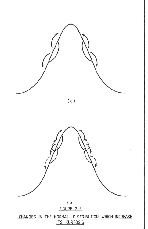
further in and some further out in such a way that the variance is unchanged but the fourth moment is increased. (See Figure 2.3(a)). The same kurtosis could be obtained by moving

different amounts of probability from different shoulder regions. (See Figure 2.3(b)). Thus if we specify the region from which the probabi ty is moved and how much is moved we are measuring nonl!ormality in a more finely

dif rentiated way than kurtosis does. The classification could be made more refined by increasing the number of regions in which the probability difference is specified. This could be increased until the density was quite closely tied down. However by keeping the number of regions as small as possible we are requiring less information to be assumed about the shape of the error distribution.

Hogg (see Hogg 1974) has developed adaptive estimators based on Q statistics such as:

(24)

( a )

( b )

FIGURE 2 · 3

[image:24.595.62.548.54.807.2]

(25)

20.

where

U(S)

is the average of the largest nS order statistics and L(S) is the average of the smallest nS order statistics. Perhaps the approach suggested above could be seen as being more in the spirit of Q statistics than of kurtos inasmuch as consideration is given directly to how the probability mass is spread rather than to a high-order moment based on this.

The aim of this study was to test the usefulness of the above method of classifying distributions. The distributions considered were piecewise linear and were constructed with regard to their general shape, their classification with

respect to the above scheme being varied systematically. "Best11 estimators were to be found and i t was hoped that these would change gradually as the distribution was changed gradually. It was also hoped that where standard distributions fitted into the scheme their 11_{best" estimators would be similar to} the estimators suggested by the classification scheme in the appropriate region. I t was believed that in this way the known results would be generalized and made more systematic.

In particular i t was hoped that the scheme would

differentiate between the double exponential distribution and the students-t distribution with six degrees of freedom.

Kurtosis fails to do this.

An advantage of the approach is that i t allows parts of the density function's shape to be varied rather than requiring the choice of a density function as a whole. This allows more flexibility in finding a distribution to match given data.

(26)

2.4 The Estimators

The estimators considered have been restricted to linear combinations of order statistics, hereafter called linear

estimators. This was largely for computational convenience, the emphasis in the st~dy being on the choice of the distri-butions. However I hope that general patterns which emerge will suggest similar patterns for other types of estimators. An advantage of considering linear estimators is that for a given distribution i t is possible to find linear

estimators of location and scale which have minimum variance in the class of unbiased linear estimators. The method for finding these best linear estimators was developed independently by Lloyd (1952) and Bennett (1952) .

In this study best linear estimators are found for the distributions described in the previous section.

2.5 The Calculations

Lloyd (1952) has shown that for a sample of size n from a symmetric distribution the best linear estimator of the mean is given by

and its variance by

02

var lJ*

=

~

where a is a scale parameter,

Q

=

B-

1, a2

B

being the covariance matrix of the order

statistics,

X is the vector of order statistics,

(27)

22.

The calculation of the best linear estimator for a distribution thus requires the calculation of the covariance matrix of the order statistics for that distribution. To

calculate the covariances for the piecewise linear distributions with finite range considered here, the regionpf integration

was broken into triangles and rectangles and Gaussian quadrature formulae for such regions were used. The calculations are exact apart from roundoff error.

Sample sizes 4, 8 and 16 were considered and details of the distributions and results are given in the appendices. Analysis of the results will concentrate on sample size 8. The distributions considered were non-zero on only a finite range. It was believed that for small sample sizes the results would not be much different from the results for

distributions which are similar except for having infinite tails. To test this, approximations having finite range were made to several standard distributions and the results compared to the known results for these distributions.

For example the standard normal density was approximated by a density which was non-zero between ±4•68. The best

linear estimator was calculated for sample sizes, N, of 8 and 16.

Table 2.5.1 gives the equations of the straight line. segments which make up the distribution. The Rth segment extends' from P [H] to P [R + 1] and has equation Y

=

A [R] X + B [R] .

(28)

TABLE 2.5 .1

Parameters of an Approximation to the Standard Normal Density

R p

IRI

A

IHI

B

[RI

1 -4·68363603266 0·000135639704009 0•00063528700507 2 -3·99939598088 0•00141041327633 0•0056908212723 3 -3•5001785904 0·066886011956 0•0246146369684 4 -2•99954698591 0 ·0256296321'~25 0·080199086531 5 -2·50032959544 0•07887357071 0•211030181828 6 •90070304026 0·213558391022 0·456036224121 7 -0•35001785904 0•072550753768 0·403640943487 8 0

TABLE 2.5.2

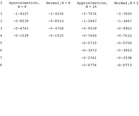
Expected Values of Order Statistics from an Approximation to the Normal Distribution and from the Normal Distribution

I Approxim<:l. tion, · Normal ,N = 8 Approximation, Normal, N

=

16

N=8 N = 16

1 -1·4227 -1·4236 -1·7631 -1·7660

2 -0·8539 -0·8522 -1·2847 -1·2847

3 -0·4742 -0·4728 -0·9928 -0·9902

4 -0·1529 -0·1525 -0·7660 -0·7632

5 -0·5719 -0•5700

6 -0·3972 -0·3962

7 -0•2341 -0·2338

[image:28.595.89.546.427.810.2]

(29)

24.

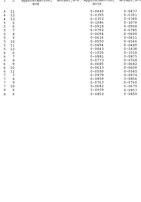
Covariances of Order Statistics from an Approximation to the Normal Distribution and from the Normal Distribution

I J Approximation, Norma1,N=B Approximation, Norma1,N=16

N=8 N=16

1 1 0·3696 0·3729 0·2937 0·2950

1 2 0.1850 0·1863 o. 14 29 0•1449

1 3 0·1257 0·1260, o. 0975 0-.0985

1 4 0.0945 0·0947 0· 0752 0•0754

1 5 0.0746 0·0748 0·0613 0··0613

1 6 0·0601 0·0602 0·0516 0. 051.6

1 7 0-0481 o.0483 0·0444 O<t0446

1 8 0.0365 0·0368 0-0388 o .. o390

1 9 o. 0 344 0·0345

1 10 0·0307 0-.0308

1 11 0·0275 Oo.0275

1 12 0·0246 0·0246

l 13 0·0220 0·0220

1 14 o.0193 0·0195

1 15 0-0166 0·0169

1 16 0·0137 0·0138

2 2 0.2385 0·2394 0.1710 0·1744

2 3 0.1635 0.1632 0·1173 0·1191

2 4 0.1236 0.1233 0·0908 0·0914

2 5 0.0978 0 •. 09 76 0·0742 0·0745

2 6 0.0790 0.0787 o.0625 0 ·0628

2 7 0.0632 0.0632 0-0538 0·0542

2 8 0·0471 0 ·0 4 7 5

2 9 0·0417 0·0421

2 10 0·0372 0 .o 375

2 11 0·0334 0 ·0 336

2 12 0·0299 0 ·0 300

2 13 0·0267 0 ·0268

2 14 0·0235 0·0237

2 15 0•0202 Oq0206

3 3 0·2020 o~2oos 0·1351 0·1363

3 4 0.1533 0.1524 0·1048 0·1049

3 5 0.1217 0·1210 0·0857 0•0855

3 6 o.0984 0·0978 0•0723 0·0722

3 7 0·0623 0 • 0 6 24

3 8 0•0546 0·0547

3 9 0•0484 0•0484

3 10 0•0432 0•0431

3 11 0•0387 0·0387

3 12 0 ·0 34 8 0·0346

3 13 0·0310 0•0309

3 14 0•0272 0·0274

4 4 0·1883 0.1872 0 ·1186 0•1179

4 5 0·1500 0·1492 0 ·09 72 0·0962

4 6 0 •0 8 21 0·0813

4 7 0 ·0708 0•0703

4 8 0 •06 20 0·0617

4 9 0 •054 9 0•0547

(30)

TABLE 2.5.3 (continued)

I J Approximation, Norma1,N=8 ,Approximation, Norma1,N=16

N=B N=16

4 11 0•0440 0·0437

4 12 0·0395 0·0391

4 13 0·0352 0·0349

5 5 0·1086 0·1074

5 6 0·0918 0·0908

5 7 0•0792 0·0785

5 8 0·0694 0•0689

5 9 0·0616 0•0611

.5 10 0·0550 0•0546

5 11 0·0494 0•0489

5 12 0·0443 0 <l438

6 6 0·1020 0 ·1010

6 7 0·0881 0·0875

6 8 0·0773 0·0768

6 9 0·0685 0·0682

6 10 0·0613 0·0609

6 11 0·0550 0·0545

7 7 0·0979 0·0974

7 8 0·0859 0·0856

7 9 0·0763 0·0760

7 10 0·0682 0·0679

8 8 0·0959 0•0957

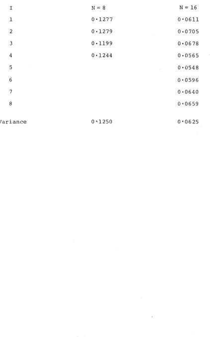
[image:30.598.81.540.107.763.2]

(31)

TABLE 2.5.4

Coefficients and Variances of Best Linear Estimators of Location for an Approximation to the Normal Distribution

I N==8 N == 16

1 0•1277 0·0611

2 0•1279 0·0705

3 0·1199 0•0678

4 0•1244 0·0565

5 0•0548

6 0•0596

7 0·0640

8 0•0659

Variance 0.,1250 0•0625

[image:31.595.93.516.128.806.2]

(32)

Table 2.5.4 gives the coefficients of the best linear estimators.

In each table values omitted may be found from considerations of symmetry.

The percentage difference from the coefficients the sample mean is always less than 4·1% for N

=

8 and 12·8% for N

=

16. Approximations to other distributions yielded

similar results. The agreement seems close enough to support the use of piecewise linear distributions in seeking overall trends in the way the best linear estimator varies as the shape of the distribution varies.

The close agreement of the variance of the es~imator

with that of the mean on the normal distribution is encouraging. This suggests some robustness in the sense that small changes in the coefficients of the estimator and in the distribution do not much affect the variance of the estimator.

2.6 Analysis of the Results for N

=

8

Forty-seven distributions were constructed, almost all having high tails. Each had variance one and was clas fied, firstly, according to where its density was above, and where below, the standard normal density. To this end two

"cutpoints" are ven. For the high-tailed distributions the region between the two cutpoints, and the corresponding region on the other side of the mean, are the regions where the

density is less than the normal density. (For the low-tailed distributions these are the regions where the density is

eater than that of the normal density). Of course, since

(33)

28 .

. the high-tailed distributions have densi es less than the normal density in the extreme tails but this factor was considered negligible for small sample sizes.

Table 2.6.1 shows the cutpoints for the 47 distributions. For given values {in standard deviations) of the left cutpoint on the ght-hand side of the distribution, and the distance apart of the two cutpoints,the number of distributions

considered is given. The positions at which various standard distributions t in are also given. Note that all values given for cutpoints are approximate.

Let us now examine some of the results for N = 8 for long-tailed distributions in the four series in which the cutpoints are distance 2 apart. A summary of these results is given in Tables 2.6.2, 2.6.3, 2.6.4 and 2.6.5. The full results are given in the appendices.

In any one series the distributions have the same cutpoints. Within the es they are classi according to the difference between the prob ility mass of the distri-bution and that of the normal distridistri-bution between the

cutpoints. It was decided to concentrate on these three parameters (the two cutpoints and this probability difference) in classifying distribution shapes as i t was found in practice that these three parameters went a good way towards tying down the approximate shape of the density function. In each series the first distribution has the maximum probability difference possible for a syrnn1etric densi each whose halves is

monotonic and which has the given cutpoints. Within each

(34)

TABLE 2.6.1

The Number of Distributions Considered for Each Pair of Cut-points and the CutCut-points for Various Standard Distributions.

Separation of the cutpoints

Left Cutpoint 1•0 1•25 1·5 1•75 2 2•25

0•25 3 6 2

0·5 9 D.E.

0•75 2 8 S.t. 6 10%CN 3

1•0 4 5% CN

1•25 2

1·5 2

The categories into which various standard distributions most nearly fit {after being scaled to have variance one) are indicated. S.t. refers to the students-t distribution with 6 degrees of freedom, D.E. to the double exponential distri-bution, 10% CN to the standard normal distribution N(O,l) with 10% contamination from N{0,9) and 5% CN to N{O,l) with 5%

[image:34.595.88.538.142.326.2]

(35)

30.

TABLE 2.6.2

The Coefficients W[I] and Variances of the Best Linear Estima-tors for N

=

8 for Some Distributions Having Cutpoints 0•25 and

2•25.

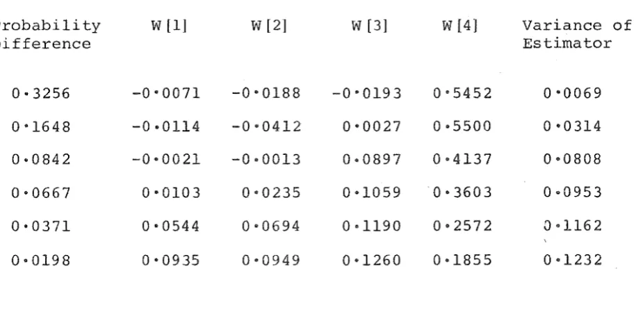
Probability Difference

0·3256 0•1648 0·0842 0•0667 0•0371 0·0198

w

[1]

-0•0071 -0·0114 0•0021 0•0103 0•0544 0•0935

w

[2]

-0•0188 0•0412 -0·0013 0•0235 0•0694 0•0949

TABLE 2.6.3

W[3] W[4]

-0·0193 0·5452 0•0027 0·5500 0·0897 0•4137 0•1059 0•3603 0·1190 0•2572 0•1260 0•1855

Variance of Estimator

0•0069

0•0808 0·0953 0•1162 0•1232

=

2·5.

Probability

w

[1]

w

[2]

w

[3]

w

[4·] Variance of

Difference Estimator

[image:35.595.96.554.150.381.2]

(36)

TABLE 2.6.4

=

2·75.

Propability

w

[1]

w

[21

w

[3]

w

[4] Variance of

0"2055 -0·0163 0•0362 0•3006 0•1796 0•031'9 0•1679 -0•0198 0·0417 0•2910 0·1871 0•0420 0•1091 -0·0210 0•0661 0•2359 0•2190 0•0617 0•0795 -0•0188 0•0908 0•2083 0•2197 0•0785 0•0410 0·0004 0·1290 0-1595 0•2111 0•1039 0·0172 0·0502 0•1509 0•1444 0·1545 0•1206

TABLE 2.6.5

=

8 for Some Distributions Having Cutpoints 1 and 3.

0•1484 0·0861 0•0473 0•0263

w

[1]

-0•0190 -0·0203 -0·0066 0·0194

w

[2]

0•1168 0·1659 0•1854 0·2087

w

[3]

0·2860 0. 2 24 8 0•1853 0·1516

w

[4]

0·1162 0·1296 0•1358 0·1202

(37)

32.

On the whole the best estimators change reasonably

smoothly both within a given series and from series to series.

Within each series the estimator moves gradually towards

mean as the probability difference decreases. In moving from

series to series as the envelope between the cutpoints is

gradually moved outwards, the weight in the best estimator

gradually moves outwards.

Consider the series with cutpoints 0•25 and 2•25. The

best near estimator for the most nonnormal distribution

(i.e. the distribution with maximum probability difference) is

very heavily weighted to the middle1 with all coefficients other

than the middle pair being negative. As the probability

difference is reduced the weight moves out from the centre and,

with one small exception, the coefficients move monotonicly

towards 0•125.

Consider the series with cutpoints 0•5 and 2•5. Here

the best estimator for the most nonnormal distribution is not

quite so heavi weighted towards the middle,with the second

pair from the middle now receiving significant weight.

Aqain, as the probability difference is reduced, the weight

moves out towards the extremes. Some coefficients do not

change monotonicly towards 0•125 but deviations from this

pattern are small. Some such deviations are not surprising.

For example the increase in W [3] away from 0 •,125 could be

considered as being caused by the rapid movement of weight

outward from the very middle pair of order statistics in order

to bring these middle coefficients closer to 0•125.

Consider the series with cutpoints 0•75 and 2•75. By

(38)

for the most nonnormal distribution, the central pair of order statistics no longer receive the maximum weight. Again as the distribution becomes closer to the normal distribution the estimator becomes closer to the mean, the weight moving out to the extremes.

Consider the series with cutpoints 1 and 3. The weight for the most nonnormal distribution has moved a little further out. Again the general trend within the series is for the weight to move out and for the estimator to get closer to the mean as the distribution becomes more like the normal

distribution.

Thus we see that there is an overall trend for weight to move outwards from the centre as the cutpoints move outwards. There is also a trend for the weight to move outwards as the distribution becomes more like the normal distribution, so that the estimators become more like the mean. Despite this trend individual coefficients do not always move monotonicly towards 0·125. Often the very middle coefficient W[4] moves slightly away from 0•125 before moving towards it. Further i t often happens that as the weight moves out to the extremes i t is not evenly distributed at st so that W[2J, for example, increases beyond 0 •125 while W[l] still carries little weight.

However too much significance should not be attached to small changes in the weights because these may be affected somewhat by the particular distribution chosen with the given cutpoints and probability difference. Rather the results should be used to show overall trends in the best estimator as the shape of the d tribution changes.

(39)

34.

other series of distributions considered (as can be seen from an examination of the appendices) .

Two pairs of similar distributions ((4,4) and ~~5),~,3)

and 0,4)) were considered in order to see whether small changes in the distribution made much difference to the best estimator, and thus to further test the continuity or the pattern in the results as the distribution is changed. Examination of the results in the appendices shows that the changes made very little difference. The main difference between the

distributions in each pair is that one is non-zero until

further out than the other. That this made little difference to the results suggests that the use of distributions which are non-zero on only a finite range does not affect the results seriously.

We now consider two distributions for which the best linear estimators for N

=

8 are known and see how closely these estimators agree with the estimators for the categories into which these distributions most nearly fit.

The normal distribution N(O,l) contaminated with 10% N(0,9) and scaled to have variance l

(i.e. 0·9 N(O,

1: 8) + 0•1 N(O, 1: 8)) has cutpoints 0•785 and 2•76 and probability difference 0·056 (approximately). The series into which i t most nearly fits is the one with cutpoints 0•75 and 2·75. Its probability difference falls between the 0·0795 and 0·0410 values considered in that series. Table 2.6.6 shows the best linear estimators and their variahces

for these distributions along with those of the 10% contaminated normal distribution itself (taken from Gastwirth and Cohen

(40)

TABLE 2.6.6

=

8 for the 10% Contaminated Normal Distribution and two Nearby Distributions with Cutpoints 0·~5 and 2•75.

0•041 (10%CN) 0·056 0•079

w

[1]

0•0004 -0.0120 -0•0188

w

[2]

0•1290 0·1275 0•0908

TABLE 2.6.7

w

[3] W[4] Variance of ·Estimator

0•1595 0•2111 0•1039 0·2016 0·1829 0·0957 0·2083 0•2197 0•0785

=

8 for the 5% Contaminated Normal Distribution and two Nearby Distributions with Cutpoints 1 and 3.

0•026 (5%CN) 0·035 0·047

w

[1]

0•0194 0·0050 -0·0066

w

[2]

0•2087 0·1708 0•1854

w

[3]

0•1516 0·1690 0•1853

w

[4]

0•1202 0·1551 0•1358

(41)

36.

The agreement between the 10% CN case and the other two distributions seems reasonably good, three of the four co-efficients and the variance for the 10% CN case being between the corresponding values for the other two distributions.

The normal distribution N(O,l) contaminated with 5% N ( 0, 3) (i.e. 0 • 9 5 N ( 0,

1: 4) + 0 · 0 5 N ( 0, 1: 4) ) has cutpoints

0•845 and 2•96 and probability difference 0·035 (approximately). Of the fuller series the one into which i t most nearly fits

is the one with cutpoints 1 and 3. Its probability difference falls between the 0·0263 and 0•0473 values considered in that series. Table 2.6.7 shows the best linear estimators and

their variances for these distributions along with those of the 5% contaminated normal distribution itself. Again the agree-ment between the 5% CN case and the other two distributions

seems reasonably good.

Thus, from the somewhat limited evidence considered,it seems that results from standard distributions are reasonably similar to those obtained from the classification scheme.

Further, as we saw earlier, the results from the classification scheme vary reasonably smoothly and cover a wide range of

distributions. Thus i t seems that the classification scheme provides a generalization of known results.

The Double Exponential Distribution and the Students-t Distribution with Six Degrees of Freedom.

(42)

this: both distributions have the same kurtosis although the asymptotically best linear estimators for the two distributions are quite differentt with the estimator for the double

exponential distribution being more heavily weighted towards the centre than that for the students-t distribution.

The cutpoints for the double exponential distribution (scaled to have variance one) are 0•485 and 2•34 and the prob-ability difference is 0•071 (approximately). The nearest distribution to this in the system is that with cutpoints 0•5 and 2•5 and probability difference 0•092. The cutpoints for the students-t distribution with 6 degrees of freedom (scaled to have variance one) are 0•705 and 2•51 and the probability difference is 0•035 (approximately}. The nearest distribution to this in the system is that with cutpoints 0•75 and 2·5 and probability difference 0•041. Table 2.6.8 shows the best linear estimators and their variances for these two distributions.

The two estimators are significantly different.

Furthermore the estimator for the distribution near the double exponential distribution has signi cantly more weight in the middle than does the estimator for the distribution like the students-t distribution. Thus i t seems that the classifica-tion system, unlike the kurtosis, is successful in distinguishing hetween the 2 distributions.

It is worth noting that a piecewise linear approximation was made to the double exponential distribution directly.

'I'he coef cients of the best linear estimator for N

=

8 were given by:

(43)

2.6.8 for the distribution near the double exponential distribution in the classification system.

A Simplification of the Classification Scheme

38.

It seems that a reasonable idea of the estimator to use on a distribution can be obtained using the two cutpoints and the probability difference. Is i t possible that a good

approximation to the estimator can be obtained if, instead of using both cutpoints, we use only their midpoint (i.e. of the cutpoints on one side of the distribution) and ignore how far apart they are? i.e. is i t possible that the estimator

depends on what the probability difference is and where i t is centred and not much on how spread out i t is?

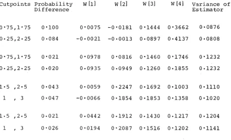
To test this, four pairs of distributions were

considered. For the two distributions in each pair, the mid-points of the two cutmid-points on the right (left) side of the distribution are the same and the probability differences are similar but one of the distributions has its outpoints

distance 1 apart and the other has them distance 2 apart. Table 2.6.9 shows the best linear estimators and their· variances for these distributions.

In each pair the best linear estimators and their

variances are fairly similar. Thus i t seems that a good idea of the best estimator to use can be obtained using only the midpoint of the cutpoints and the probability difference. It would be worthwhile to test this hypothesis over a wider range of distributions.

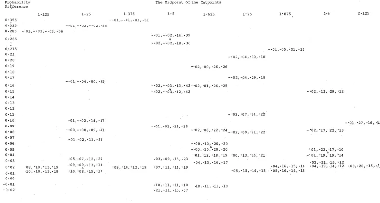
Table 2.6.10 shows the best estimators for the distri-butions organized with respect to these two parameters.

(44)

TABLE 2.6.8

=

8 for a Distribution Near the Double Exponential Distribution and a Distribution Near the Students-t Dis

bution with 6 Degrees of Freedom.

Cutpoints Probability

w

[1]

w

[2]

w

[3]

w

[4] Variance of

0•5 ,2•5 0•092 -0·0135 0·0124 0•1495 0·3516 QoQ77Q 0•75,2·5 0·041 0·0108 0·1203 0·1797 0·1892 0<>1098

Note that the rst distribution is close to the double exponential distribution and the second to the students-t

(45)

40.

TABLE 2.6.9

=

8 for 4 Pairs of Distributions Where in Each Pair the 2 Distributions Have Cutpoints Centred About the Same

Point and Have Similar Probability Differences.

Cutpoints Probability Difference

0•75,1•75 0·25,2·25

1•5 ,2·5 1 , 3

1·5 ,2·5 1 1 3

0•100 0·084

0•021 0·020

0•043 0•047

0·021 0•026

w

[1]

w

[2]

w

[3] W[4] Variance of Estimator

0•0075 -0·0181 0•1444 0•3662 -0·0021 -0·0013 0·0897 0•4137

0•0978 0•0816 0•1460 0•1746 0·0935 0·0949 0·1260 0·1855

0·0059 0•2247 0•1692 0•1003 -0•0066 0·1854 0•1853 0•1358

0·0442 0·1912 0·1430 0·1217 0·0194 0·2087 0•1516 0•1202

0·0876 0·0808

0•1232 0·1232

0•1110 0•1020

[image:45.595.87.563.167.454.2]

(46)

Probability

Di~ference

0·355

_..

0.325

1·125

0·285 -·01,-;03,-·03,·56

1·25

-· 01,-. 02,-· 02, ·55

Forty-ssven Dis tributions

The Midpoint of the Cutpoints

1·375 1·5 1·625 1•75

-·01,-·01, ·01, ·51

-·01,-·02, •14, ·39 &

0·265 -·02,-·02,·18,·36

d·215 0·21 0•20 0·19 0·18 0•17 0·16 0•15 0•14 0·13 0·12 0•11 0•10 0·09 0·08 0·07 0·06 0·05 0•04 0·03 0'02 0·01 0•00 -0·01 -0·02

·o8, ·10, ·13, ·19 ·10. ·10. ·13. ·18

-·01,-·04, •00, ·55

·01,-·02,•14,·37

-·00,-·00,•09,·41

-01, • 0 2 •• 11, • 3 6

·05' ·07' ·12, ·26

·09, ·09, ·13, ·19 &

•10, •OS, •15, •17

•09, •10, •12, •19

-·02, ·00, ·26, ·26

-. 02' -·03. ·13' •42- ·02. •01, •26. •25 . &

-·02,-·03, •12, ·42

-·01, ·01, ·15, •35

-·02, ·04, •30, ·18

-·02,·04,•29,•19

- •02' •07' •24' ·22.

-·02, •06, •22, •24 -·02, '09, •21, •22

·03, ·09, ·15, ·23

•07,•11,•14,•19

·18, ·11, •11, ·10 ·21, ·11, ·10, •07

-·oo, ·1o, ·20, ·2o & -·00, •10, •20, •20

•01, •12, •18, •19

·04, ·13, ·16, ·17

·18' ·11' ·11' •10

·oo, ·13, ·16, ·21

·o5, ·15, ·14, ·15

1•875

-·01, •05, ·31, ·15

·04, ·16, ·15, ·16 ·05, •16, •14, •15

2·0

- •02, •12' •29 1 •12

-"02, "17, •22, •13

• 01, •22, •17. •10 & -· 01, •19' "19. "14

•02, ·21, •15, •12 ·04. ·19' •14. ·12

2•125

-·o1, ·27 I ·161 ·o8

[image:46.844.36.811.107.520.2]

(47)

parameters determine the best linear estimator for a distribution.

42.

The most obvious patterns are that weight moves out from the centre as one moves down the table or to the right of

the

table. At the top left of the table the estimators are very heavily weighted towards the centre. We see that W[4] tends to decrease going down a column and going to the right. Far enough to the righ~weight has moved from W[4] to the extent that i t is no longer the biggest coefficient. Thus going down these columns W[4] may increase at first, as weight from the bigger coefficients further out is distributed more evenly. Going down these columns we find a fairly smooth decrease in whichever coefficient is biggest at the top of the column.

Why does weight move out from the centre as one moves down or to the right of the table? Perhaps the reason is that, as we shall consider further in Chapter 4, the higher the

probability density is in a region,the more weight should go to observations likely to fall there. Thus when the probability difference is large, and consequently the probability density is high in the middle, weight is given to the middle observa-tions. Further the narrower this central region of high density is, the further the weight must go to the middle in order to take advantage of i t .

It is worth noting how useful the "second" variable, the midpoint of the cutpoints, is in determining the best

estimator. The changes in the best estimator going across the table are regular and quite strong. The usefulness of the probability difference is also clear - for example the

(48)

are much closer to the mean than those for distributions with big probability differences.

Overall the best estimator changes reasonably smoothly as one moves through the table so that the position of a

distribution in the table approximately determines its best estimator.

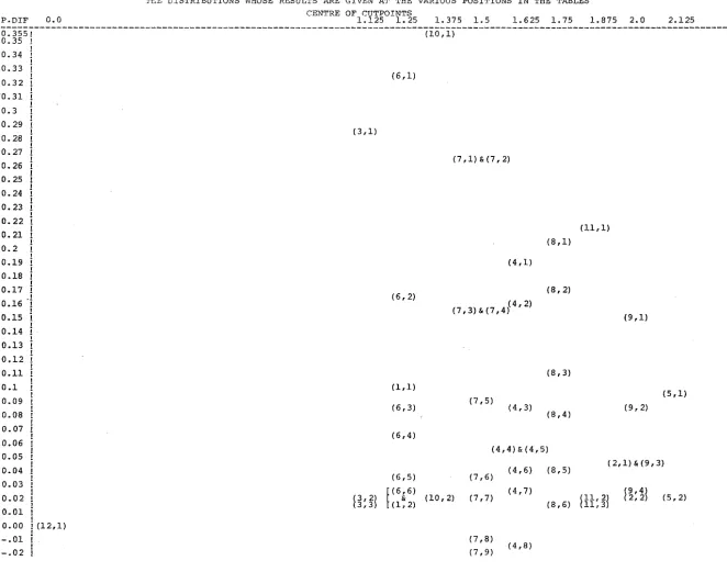
Estimabili

We saw earlier that the normal distribution is the least estimable distribution. Examination of the results in the appendices shows that, further, the more nonnormal a distri-·bution is the more estimable i t is: within any one series of

high-tailed distributions the greater the probability

difference the smaller the variance of the best linear estimator. This pattern is also shown in Table 2.6.11 which shows the variances of the best estimators at different places

within the classification scheme. The variance of the best linear estimator changes reasonably smoothly as the classifica-tion of the distribuclassifica-tion changes. In fact the variance of the best linear estimator is fairly well determined by the probability difference, which serves as a rough measure of non-normality. The main exception is the second of the pair of distributions with probability difference between 0•26 and

0·27. I t should be noted that this is an unusual distribution whose density is made of three horizontal straight lines.

Table 3.1.1 shows which distributions the figures in Table 2.6.11 refer to.

Low-tailed Distributions

(49)

TABLE 2.6.11

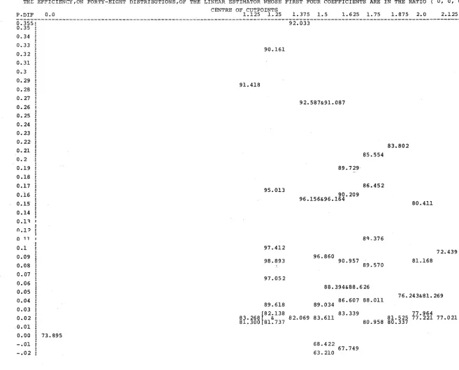
THE VARIANCE OF THE BEST LINEAR ESTIMATOR FOR FORTY-EIGHT DISTRIBUTIONS CENTRE OF CUTPOINTS

P.DIF 0.0 1.125 1.25 1.375 1.5 1.625 1;75 1.875 2.0 2.125

a~355!---a~ao4

________________________________________________ _

0.35 0.34 0.33 0.32 0.31 0.3 0. 29 0.28 0.27 0.26 0.25 o. 24 o. 23 0.22 0.21 0.2 0.19 0.18 0.17 0.16 0.15 0.14 O.l 3 0.1? 011 0.1 0.09 o.na 0.07 0.06 o.os 0.04 0.03 0.02 0.01

I

0.00 i I

-.01 -.02

0.007

0.015

0.031

0.088

0.081

0.095

0.116

r o.123 0.122f & 0.124 0.123

0.125

0.016& 0.028

0.039

0.045 0.043& 0.044

0.077

0.076

0.032

0.042

0.062

0.079

0.101& 0.103

0.123

0.113

0.121

0.124 0.121

0.110 0.104

0.119

0.121

0.123

0.029

0.054

0.075 0.076

0.111& 0.102

0.114

(50)

study of low-tailed distributions. However examination of the results for the three that were studied (Distributions

(5,8),t8,8)and (8,9)) suggests that for low-tailed distributions extra weight should be placed on the extreme observations and less weight on the central observations.

Conclusion

(51)

CHAPTER 3

THE ROBUSTNESS OF LINEAR ESTIMATORS ON NEAR-NORMAL DENSITIES OF VARIOUS SHAPES

46.

3.1 Introduction

An estimator considered robust if its performance is good not only for a given error distribution but also for

distributions which are similar to the given one. In Chapter 2 an attempt was made to organize the set of distributions systematically and to find a set of tures of a distribution which are useful for determining a good estimator to use on i t .

In this chapter consideration is given to the robustness of linear estimators over sets of distributions organized in this way.

Emphasis is placed on the choice of a measure of

quali An estimator's quality is measured firstly by its e ciency relative to the best linear estimator and secondly by its variance when each distribution is scaled to have

variance one. The results obtained using these two measures are compared and a third measure of quality is suggested as being better. Using this measure an assessment of the

robustness of the estimators is made and, in the light of this, the value of efficiency as a measure is reconsidered.

The distributions considered are the same ones as were considered in Chapter 2 including the approximation to the normal distribution given in Section 2.5. Results are

(52)

Section 2.6 for describing the shape of a density (i.e. the probability difference between the cutpoints on one side and the midpoint of the cutpoints on one side). Table 3.1.1

shows which distributions occupy which places in these tables.

3.2 Robustness of Efficiency

'rhe robustness of efficiency of linear estimators will now be considered. Efficiency is defined as (variance of best available estimator/variance of estimator) and in this secti6n the best available estimator for a distribution is taken to be the best linear estimator. The use of efficiency as a measure is common in robustness studies.

Forty-one estimators were considered for sample size eight but the results are given only for some of these

(including the best ones) . In considering the robustness of an estimator emphasis should be placed on distributions in the lower group in the tables (i.e. with probability differences less than about .11) as the other distributions are probably unrealistic, being ext~emely nonnormal. However these extreme distributions are interesting in that they help to reveal overall trends.

The estimators discussed have weights (W[l}, W[2] , ••. , W [8] ) with W [I} = W [9 - I} and with (W [11 , W [2] , W [3] , W [4] ) in

the ratios: (0,0,0,1), (0,0,1,2), (0,0,1,1), (0,1,2,2), (0,1,1,1), (1,1,2,4), (1,1,2,2), {1,1,1,1), (-1,2,15,10} and

(53)

P.DIF 0.0

0.355! 0.35

0.34

0.33

0.32

0.31

0.3 0.29

0.28

0.27

o. 26

o. 25 0. 24

o. 23 0.22 o. 21 0.2

0.19

0.18 0.17

0.16

0.15

0.14

0.13

0.12

0.11

0.1

0.09

0.08

0.07

0.06 0.05

0.04

0.03

0.02

0.01

0.00 (12,1) -.01

-.02

TABLE 3.1.1

TEE DISTRIBUTIONS WHOSE RESULTS ARE GIVEN AT THE VARIOUS POSITIONS IN THE TABLES CENTRE OF CUTPOINTS

1.125 1.25 1.375 1.5 1.625 1.75 1.875 2.0 (10,1)

{6, 1)

( 3 ,1)

{7,1}&(7,2)

(11,1)

{ 8, 1)

( 4, 1)

(8, 2) (6, 2)

( 7, 3) & {7, 4 ){ 4, 2)

(9 ,1)

(8, 3)

(1,1)

(7 ,5)

(6, 3) ( 4, 3)

( 8, 4) (9, 2)

{6 ,4)

(4,4) & {4,5)

2.125

( 5, 1)

( 4, 6) (8 ,5) (2,1) &(9,3) {6, 5) (7, 6)

~ (6&6) ( 4, 7) f9, 4!

f3, 2J _3,3 _{(1, 2)} ( 10, 2) (7, 7) _{(8, 6)}

lll,

_11,32i 2,2 (5, 2)

(7, 8)

[image:53.842.73.735.49.570.2]