ISSN 1173-5996
Assessing the Feasibility of Reducing
the Grid Resolution in FDS Field
Modelling
by
Nathaniel Mead Patterson
Supervised by:
Dr Charley Fleischmann
Fire Engineering Research Report 02/12
May 2002
This report was presented as a project report as part of the ME (Fire) Degree at the University of Canterbury
School of Engineering University of Canterbury
Abstract
Field modelling is increasingly becoming the main form of fire modelling for design purposes. To reduce the computational running time of field models designers are sacrificing fine grid resolution without considering the consequences this could incur on the results. This report aims to provide some validation on the extent to which grid size can be increased in the field model Fire Dynamics Simulator (FDS) before the results are compromised and to determine whether there is a point at which zone model predictions become more reliable.
FDS model predictions using a range of grid sizes were compared against two separate sets of experiments:
1. The University of Canterbury McLeans Island tests. These tests were performed using two isorooms, each measuring 2.4 x 3.6 x 2.4 metres. 55kW and 110kW tests were simulated in FDS.
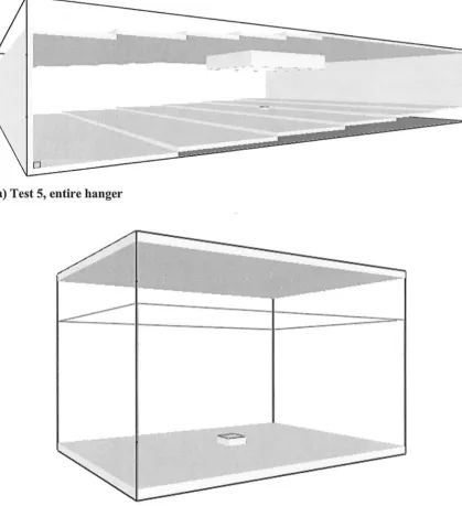
2. The US Navy Hanger tests in Hawaii. The hanger measured 98 x 74 metres x 15 metres high at its apex. Two tests were simulated in FDS. These had Heat Release Rates (HRRs) of 5580kW and 6670kW respectively. The second test had a draft curtain situated centrally around the fire. This was modelled in two different FDS constructions; one simulated the entire hanger, the other only the area of the draft curtain.
Simulations using the zone model CF AST were also performed for all the tests outlined above.
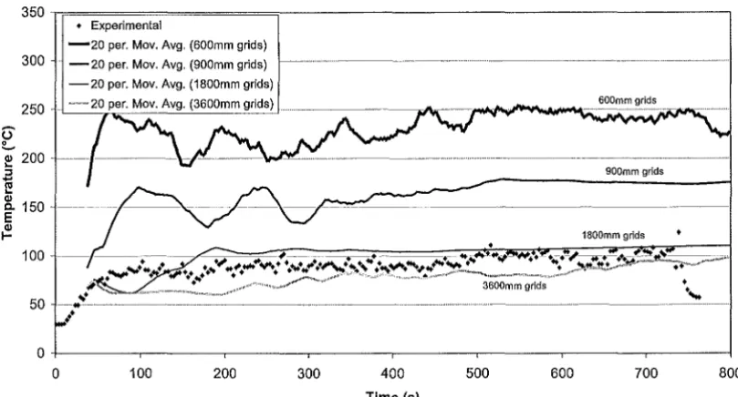
The simulations of the Hawaii hanger tests gave very unreliable temperature predictions in the fire plume; the model with 600mm (H/25) grids over-predicted the temperatures by about 150°C. Over-predictions of as much as 60°C were also observed in the temperature predictions within the confines of the draft curtain. These large discrepancies were due to the poor modelling of the high degree of turbulence that occurred in these areas. Locations away from the fire plume or outside the draft curtain gave much better predictions because turbulence was less. In these regions grid sizes of up to 1800mm (H/8) still gave similar accuracy to the 600mm (H/24) grid models. The model using 3600mm (H/4) grids began to display some inaccuracy in the temperature gradients it predicted. The zone models made much better predictions for the temperatures within the draft curtain. This was due to the relatively steady state nature and uniform temperatures that existed there. It was difficult to compare the zone models to the main hanger space because of the limited experimental data that was provided.
Acknowledgments
I would like to thank the following people for their assistance and support in helping me to complete this project:
• My supervisor, Dr Charley Fleischmann.
• The New Zealand Fire Service Commission for their financial help and continued support of the M.E. Fire program.
• Mike Spearpoint for his advise and patience with my problems in spite of the fact that he was not my supervisor.
• Tom and Donna, who each read various sections of the report when required and Dad, who waded through the final draft.
• Mr Peter Coursey and Mr Joost Stenfert-Kroese for providing prompt computer services and the facilities with which to work with.
Table of Contents
Abstract ... i
Acl{nowledgments ...•... iii
List of Figures ... xi
List of Tables ... xix
Glossary of terms ... xxi
1 Introduction ... 1
1.1 Overview ... 1
1.2 Fire modelling ... 1
1.3 Impetus for research ... 3
1.4 Research objectives ... 3
1.5 Report outline ... 4
1. 6 Limitations ... 4
2 Literature Review ... 5
2.1 Field Modelling History ... 5
2.2 Model Validation ... 7
2.2.1 Domestic sized enclosure fires ... 7
2.2.2 Large scale enclosure fires ... 9
2.3 Fire modelling for design ... 11
3 FDS model ... l3
3.1 Hydrodynamic model ... ] 3
3.1.1 Conservation ofMass ... 14
3.1.2 Conservation ofMomentum ... 14
3 .1.3 Conservation of Energy ... 15
3 .1.4 Conservation of Species ... 16
3.2 Combustion model ... .. 16
3.3 Thermal radiation model ... 19
4 McLeans Island Tests ... 21
4.1 Experimental set-up ... 21
4.2 FDS modelling ... 23
4.2.1 Grid sizes ... 24
4.2.2 Model discrepancies ... 24
4.2.3 Input variables ... 25
4.3 Zone modelling ... 26
4.4 Data analysis ... 26
4.4.1 Temperature measurements ... 26
4.4.2 Layer height ... 27
4.4.3 Upper and lower layer temperatures ... 27
4.4.4 Oxygen concentration data ... 27
5 McLeans Island Results ... 29
5.1 55kWtest ... 30
5 .1.1 Temperature tree profiles ... 3 0 5 .1.2 Layer heights ... 34
5.1.3 Upper and Lower Layer Temperatures ... 35
5.1.4 Oxygen Concentration ... 36
5.2 110kWtest ... 38
5.2.2 Layer Heights ... 42
5.2.3 Upper and Lower Layer Temperatures ... .43
5.2.4 Oxygen Concentration ... 44
5.3 Model run times ... 45
5.4 Discussion and conclusions ... 46
5.4 .1 Temperature prediction differences ... 46
5.4 .2 Floor and ceiling temperatures ... 4 7 5.4.3 Temperatures directly over the bumer ... 49
5.4.4 Temperature gradient instability ... 51
5.4.5 Layer height comparisons ... 53
5.4.6 Layer temperature comparisons ... 53
5.4.7 Oxygen concentration comparisons ... 55
5.4.8 Summary ... 56
6 US Navy Hanger Tests ... , ... 57
6.1 Experimental set-up ... 57
6.2 FDS modelling ... 61
6.2.1 Test fires ... 61
6.2.2 Grid sizing ... 65
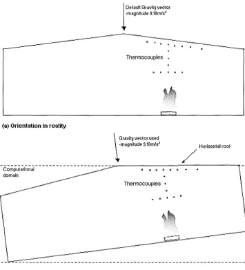
6.2.3 Inclined roof ... 66
6.2.4 Problems with gravity vector ... 66
6.2.5 Thermocouples ... 69
6.2.6 Ventilation ... 69
6.2.7 Model discrepancies ... 70
6.2.8 Input variables ... 70
6.3 Zone Modelling ... 72
6.3 .1 Test 7, entire hanger ... 72
7 US Navy Hanger Results ... 75
7.1 Test .7, en tire hanger ... 7 6 7 .1.1 Plume temperature comparisons ... 7 6 7.1.2 East thermocouple tree comparisons ... 78
7 .1.3 Zone model comparisons ... 81
7.2 Test 5, entire hanger ... 82
7.2.1 Plume temperature comparisons ... 82
7 .2.2 East thermocouple tree comparisons ... 84
7.2.3 Draft curtain results ... 87
7.2.4 Zone model comparisons ... 90
7.3 Test 5, draft curtain only. ... 91
7. 3.1 Plume temperature comparisons ... 91
7.3.2 East thermocouple tree comparisons ... 93
7.3.3 7.3.4 Draft curtain results .. .-... 96
Zone model comparisons ... 97
7.4 Model Run times ... 98
7.5 7.5.1 7.5.2 7.5.3 7.5.4 7.5.5 7.5.6 7.5.7 7.5.8 7.5.9 Discussion and conclusions ... 99
Plume temperature comparisons ... 99
Stretched grid FDS model ... 1 03 Flame heights ... 105
Mixture fraction ... 1 07 Unstable flame ... 110
Draft curtain trends ... 111
Other differences ... 113
Zone models ... 114
Summary ... 117
8 Conclusions ... 119
8.3 Overall conclusions ... 121
8.4 Recommendations ... 122
9 References ... 123
Appendix A: Differences between the FDS models and the experiments ... 127
Appendix B: Model input data files ... 131
B.1 McLeans Island input files ... . 131
B.2 Hawaii Hanger tests ... 137
Appendix C: Additional Results ... 159
C 1 McLeans Island Results ... 159
C2 US Navy Hanger Results ... 165
List of Figures
Figure 3.1: State relations for propane (McGrattan et al, 2001) ... 18
Figure 4.1: McLeans Island Isoroom illustration (reproduced from Nielsen (2000)) ... 21
Figure 4.2: Location of the thermocouple trees for the McLeans Island isorooms ... 22
Figure 4.3: Smokeview picture of the FDS isorooms using a grid size of 100mm (H/24) ... 23
Figure 5.1: Temperature profiles for Tree 1 for the 55kW fire ... 30
Figure 5.2: Temperature profile for Tree 3 (directly above the burner) for the 55kW fire ... 30
Figure 5.3: Temperature profile for the doorway tree for the 55kW fire ... 31
Figure 5.4: Temperature profiles for Tree 5 for the 55kW fire ... 31
Figure 5.5: Temperature profile for Tree 8 for the 55kW fire ... 32
Figure 5.6: Layer height comparisons between FDS, CFAST and experimental results for the 55kW fire ... 34
Figure 5.7: Upper and lower layer temperature comparisons between FDS, CFAST and experimental results for the 55kW fire ... 35
Figure 5.8: Oxygen concentration comparisons in the fire room between the FDS models and experimental results for the 55kW fire ... 36
Figure 5.9: Oxygen concentration comparisons in the front room between the FDS models and experimental results for the 55kW fire ... 36
Figure 5.10: Temperature profiles for Tree 1 for the llOkW fire ... 38
Figure 5.14: Temperature profiles for Tree 8 for the 110kW fire ... .40
Figure 5.15: Layer height comparisons between FDS, CFAST and experimental results for the
110kW fire ... 42
Figure 5.16: Upper and lower layer temperature comparisons between FDS, CFAST and
experimental results for the 110kW fire ... .43
Figure 5.17: Oxygen concentration comparisons in the fire room between the FDS models and
experimental results for the 11 OkW test. ... .44
Figure 5.18: Oxygen concentration comparisons in the doorway and the front room between
the FDS models and experimental results for the llOkW fire ... 44
Figure 5.19: Floor temperature comparisons between initial and revised FDS model results
and experimental values ... 48
Figure 5.20: Ceiling temperature comparisons between initial and revised FDS model results
and experimental values ... 49
Figure 5.21: Illustration of the flame sheet predicted by the 300mm (HIS) grid model. ... 51
Figure 5.22: Smokeview image of the temperatures near the door at a fire time of 520
seconds, showing the thermocouple that displays the anomaly (circled) ... 52
Figure 5.23: Comparison of the zone model temperature approximations with FDS and
experimental results for Tree 1 ... 54
Figure 5.24: Comparison of the zone model temperature approximations with FDS and
experimental results for Tree 8 ... 55
Figure 6.1: North and east elevations of the Hawaii hanger (not to scale) (modified from Gott
et al (1997)) ... 58
Figure 6.2: Plan view of the Hawaii hanger (Gott et al, 1997) ... 59
Figure 6.4: Hawaii hanger test fire using JP4 jet fuel in a 2 metre diameter pan (Gott et al,
1997) ... 61
Figure 6.5: FDS model of Test 7, entire hanger using 600mm (H/25) grids ... 62
Figure 6.6: Smokeview images of the FDS models that were used for Test 5 using a 600mm
(H/25) grid ... 63
Figure 6.7: Illustration showing the stretched grids for the 3600mm (H/4) FDS model. ... 65
Figure 6.8: Illustration of how the hanger orientation was specified in the FDS models ... 67
Figure 6.9: Smokeview images of the FDS models of the Hawaii Hanger, without a draft
curtain ... 68
Figure 7.1: Test 7, entire hanger; predicted time-temperature profiles for thermocouple C1,
directly above the fire, 0.3 metres below the ceiling ... 76
Figure 7.2: Test 7, entire hanger; predicted time-temperature profiles for thermocouple C12,
directly above the fire, 6.1 metres below the ceiling ... 76
Figure 7.3: Test 7, entire hanger; predicted time-temperature profiles for thermocouple E5,
9.1 metres east of the fire, 0.3 metres below the ceiling ... 78
Figure 7.4: Test 7, entire hanger; predicted time-temperature profiles for thermocouple E7,
9.1 metres east of the fire, 0.76 metres below the ceiling ... 78
Figure 7.5: Test 7, entire hanger; predicted time-temperature profiles for thermocouple E8,
9.1 metres east of the fire, 1.22 metres below the ceiling ... 79
Figure 7.6: Test 7, entire hanger; predicted time-temperature profiles for thermocouple E9,
9.1 metres east of the fire, 3 metres below the ceiling ... 79
Figure 7.7: Test 7, entire hanger; comparison of the zone model upper layer temperature
Figure 7.9: Test 5, entire hanger; predicted time-temperature profiles for thermocouple C12,
directly above the fire, 6.1 metres below the ceiling ... 82
Figure 7.10: Test 5, entire hanger; predicted time-temperature profiles for thermocouple E5,
9.1 metres east of the fire, 0.3 metres below the ceiling ... 84
Figure 7.11: Test 5, entire hanger; predicted time-temperature profiles for thermocouple E7,
9.1 metres east of the fire, 0.76 metres below the ceiling ... 84
Figure 7.12: Test 5, entire hanger; predicted time-temperature profiles for thermocouple E8,
9.1 metres east of the fire, 1.22 metres below the ceiling ... 85
Figure 7.13: Test 5, entire hanger; predicted time-temperature profiles for thermocouple E9,
9.1 metres east of the fire, 3 metres below the ceiling ... 85
Figure 7.14: Test 5, entire hanger; temperature profiles in relation to height for the
thermocouple tree 9.1 metres east of the fire at a time of 500 seconds ... 86
Figure 7.15: Test 5, entire hanger; predicted time-temperature profiles for thermocouple W1,
17.7 metres west of the fire, 0.3 metres below the ceiling, outside the draft curtain ... 87
Figure 7.16: Test 5, entire hanger; predicted time-temperature profiles for thermocouple W2,
14.6 metres west of the fire, 0.3 metres below the ceiling, outside the draft curtain ... 87
Figure 7.17: Test 5, entire hanger; comparison of the zone model upper layer temperature
profile within the draft curtain with profiles from FDS model and experimental averages .
... 90
Figure 7.18: Test 5, draft curtain only; predicted time-temperature profiles for thermocouple
C1, directly above the fire, 0.3 metres below the ceiling ... 91
Figure 7.19: Test 5, draft curtain only; predicted time-temperature profiles for thermocouple
C12, directly above the fire, 6.1 metres below the ceiling ... 91
Figure 7.20: Test 5, draft curtain; predicted time-temperature profiles for thermocouple E5,
Figure 7.21: Test 5, draft curtain; predicted time-temperature profiles for thermocouple E8,
9.1 metres east of the fire, 1.22 metres below the ceiling ... 93
Figure 7.22: Test 5, draft curtain; predicted time-temperature profiles for thermocouple E9,
9.1 metres east ofthe fire, 3 metres below the ceiling ... 94
Figure 7.23: Test 5, draft curtain; temperature profiles in relation to height for the
thermocouple tree 9.1 metres east ofthe fire at a time of500 seconds ... 95
Figure 7.24: Test 5, draft curtain; comparison of the zone model upper layer temperature
profile within the draft curtain with profiles from FDS model and experimental averages .
... 97
Figure 7.25: Comparisons of average temperatures at various heights in the fire plume for
Test 7, entire hanger ... 101
Figure 7.26: Test 7, entire hanger; predicted time-temperature profiles for thermocouple C11,
2.13 metres east of the fire, 3 metres below the ceiling ... 1 02
Figure 7.27: Plan view of a portion of the Hawaii hanger floor showing the fine grids over the
fire and plume area ... 104
Figure 7.28: Comparison of the results from the model with stretched grids for the
thermocouple at location C12 (directly above the fire 6.1 metres below the ceiling) .... 105
Figure 7.29: Smokeview images of the flames as predicted by the FDS model showing the
variation in height. ... 108
Figure 7.30: Smokeview image of the 600mm grid model showing the extent of leaning and
instability in the simulated flame over a short time span ... 111
Figure 7.31: Test 7, entire hanger; upper layer temperature comparisons using a revised
Figure C.1: Temperature profiles for Tree 2 for the 55kW fire ... 159
Figure C.2: Temperature profiles for Tree 4 for the 55kW fire ... 160
Figure C.3: Temperature profiles for Tree 6 for the 55kW fire ... 160
Figure C.4: Temperature profiles for Tree 7 for the 55kW fire ... 161
Figure C. 5: Temperature profiles for Tree 2 for the 11 OkW fire ... 161
Figure C.6: Temperature profiles for Tree 4 for the 110kW fire ... 162
Figure C. 7: Temperature profiles for Tree 6 for the 110kW fire ... 162
Figure C. 8: Temperature profiles for Tree 7 for the 11 OkW fire ... 163
Figure C.9: Test 7, entire hanger; predicted time-temperature profiles for thermocouple C2, directly above the fire, 1.5 metres below the ceiling ... 165
Figure C. 10: Test 7, entire hanger; predicted time-temperature profiles for thermocouple C3, directly above the fire, 1.5 metres below the ceiling ... 165
Figure C. 11: Test 7, entire hanger; predicted time-temperature profiles for thermocouple E4, 9.1 metres East of the fire, 0.15 metres below the ceiling ... 166
Figure C. 12: Test 7, entire hanger; predicted time-temperature profiles for thermocouple E6, 9.1 metres East of the fire, 0.46 metres below the ceiling ... 166
Figure C.13: Test 5, entire hanger; predicted time-temperature profiles for thermocouple C2, directly above the fire, 1.5 metres below the ceiling ... 167
Figure C.14: Test 5, entire hanger; predicted time-temperature profiles for thermocouple C3, directly above the fire, 3 metres below the ceiling ... 167
Figure C.15: Test 5, entire hanger; predicted time-temperature profiles for thermocouple E4, 9.1 metres East of the fire, 0.15 metres below the ceiling ... 168
Figure C.17: Zone model predictions of the layer heights in the draft curtain "compartment"
and main hanger area ... 169
Figure C.l8: Test 5, draft curtain; predicted time-temperature profiles for thermocouple C2,
directly above the fire, 1.5 metres below the ceiling ... 170
Figure C.l9: Test 5, draft curtain; predicted time-temperature profiles for thermocouple C3,
directly above the fire, 3 metres below the ceiling ... 170
Figure C.20: Test 5, draft curtain; predicted time-temperature profiles for thermocouple E4,
9.1 metres East of the fire, 0.15 metres below the ceiling ... 171
Figure C.21: Test 5, draft curtain; predicted time-temperature profiles for thermocouple E6,
9.1 metres East of the fire, 0.46 metres below the ceiling ... 171
Figure C.22: Test 5, draft curtain; predicted time-temperature profiles for thermocouple E7,
9.1 metres East of the fire, 0. 7 6 metres below the ceiling ... 172
Figure C.23: Test 5, draft curtain; zone model prediction of the layer height in the draft
curtain "compartment" showing the times that the layer reaches thermocouples E5 and
E9 ... 172
Figure C.24: Stretched grid model; predicted time-temperature profiles for thermocouple E5,
9.1 metres East of the fire, 0.3 metres below the ceiling ... 173
Figure C.25: Stretched grid model; predicted time-temperature profiles for thermocouple E8,
List of Tables
Table 4.1: Input HRRPUA and output HRRs for the McLeans Island FDS models ... 24
Table 5.1: FDS and CFAST model running times for the McLeans Island simulations ... 45
Table 5.2: Experimental and FDS model flame heights for McLeans Island isorooms ... 50
Table 6.1: Input HRRPUA and output HRRs for the Hawaii hanger tests ... 64
Table 7.1: Approximate draft curtain filling time based on the temperature rise of thermocouples immediately outside the draft curtain ... 88
Table 7.2: Test 5, draft curtain; initial temperature rise delays for thermocouples E5 and E9 . ... 96
Table 7.3: FDS and CFAST model running times for the Hawaii hanger simulations ... 98
Table 7.4: Average temperatures for Test 7, at thermocouple Cl2 (directly above the fire, 6.1 metres below the ceiling) ... 100
Table 7.5: Flame height comparisons ... 106
Table 7.6: Comparison between FDS models when the mixture fraction correction is turned off and on ... 11 0 Table A 1: Discrepancies in the FDS model when modelling the McLeans isorooms ... 127
Table A 2: Discrepancies in the FDS model when modelling the entire hanger ... 128
Table A 3: Discrepancies in the FDS model when modelling the draft curtain only ... 129
Acronyms:
BRANZ CFAST CFD DNS FDS HRR HRRPUA LES NIST RAM RTE
FDS input calls:
ALPHA
C DELTA RHO DELTA
KS TMPA
Nomenclature:
c
Glossary of terms
Building and Research Association of New Zealand
Fire And Smoke Transport; the zone model used in this research Computational Fluid Dynamics
Direct Numerical Simulation
Fire Dynamic Simulator; the CFD model used in this research Heat Release Rate
Heat Release Rate Per Unit Area Large Eddy Simulation
National Institute of Standards and Technology Random Access Memory
Radiative Transport Equation
thermal diffusivity
product of specific heat, thickness and density obstruction thickness
It, k L p q"' Q* Q Qc T t
u=(u,
v,
w)W/"
z
z
Zr Zr,eff
HRR per unit mass of oxygen consumed centreline plume temperature above ambient external force vector (sprinkler droplet drag) acceleration of gravity
enclosure height
enthalpy; heat transfer coefficient enthalpy of Ah species
radiation intensity
radiation blackbody intensity
thermal conductivity, turbulent kinetic energy Flame height
molecular weight of Ah gas species oxygen consumption rate
pressure
radiative heat flux vector
heat release rate per unit volume Dimensionless HRR
total heat release rate convective heat release rate temperature
time
velocity vector
production rate of Ah species per unit volume mass fraction of fuel
mass fraction of fuel in the fuel stream mass fraction of Ah species
mass fraction of oxygen
mass fraction of oxygen in ambient height above fire base
virtual origin of fire mixture fraction
ox
E
K
a
Xr
00
a a a
+ +
-ax ay az
nominal grid size
viscous dissipation energy absorption coefficient dynamic viscosity density
Stefan-Boltzmann constant viscous stress tensor stoichiometric coefficient local radiative loss fraction
1
Introduction
1.1
Overview
Fire Engineering is a continually expanding and complex multi disciplinary field. As this field expands and awareness of the role of fire engineering develops there is an increasing need for more case specific design solutions (Buchanan (Ed.), 2001). Fire engineering therefore is increasingly moving towards performance-based codes and away from the more restrictive prescriptive codes. A performance-based code is a much more rational and effective approach, giving scope to designers to use specific fire engineering design to arrive at a solution to a problem. New Zealand was the first to introduce a performance based code for fire engineering in 1992 and has been closely followed by Sweden (1994) and Australia (1996), with the USA currently in the process of introducing it (Buchanan (Ed.), 2001).
With the need for case specific design solutions the use of fire modelling techniques has become widely used in industry. This has fuelled the development of more and more complex fire models. It began with the introduction of zone models and progressed onto the development of the more complex field models over the last ten years (Collier, 1997). However, the use of fire modelling as a quantitative solution cannot be achieved without some sort of validation of the model that shows that it can perform satisfactorily in a wide range of scenarios. This is the main drive of this research.
1.2
Fire modelling
power, actual computer modelling of fires has only just come to fruition in the last 20 years (Mawhinney et al, 1994).
The two approaches to fire modelling are: 1) probabilistic and 2) deterministic (Stroup, 1995). Probabilistic models make a risk based assessment of what could happen in a particular scenario based on experience and past occurrences of fires. Deterministic models on the other hand provide a more rigorous mathematical approach to modelling based on physical laws (Kanury, 1987). Many phenomena in classical physics are explained using deterministic models. For example, Newton's laws of motion are deterministic models. The modelling of fire behaviour, although vastly more complicated, naturally leads on from some of the classical physics equations such as those for fluid dynamics.
Deterministic fire models can range from quite simple correlations that utilise only a few equations to highly complex models requiring hours of computer time (Stroup, 1995). These models are generally divided into two types, zone models and field models. Both models are deterministic models ofvarying complexities (Kanury, 1987).
The zone model is the simpler of the two and has been widely used as a design tool in fire engineering for many years. The model simply represents the enclosure as two distinct homogenous zones: a hot upper layer and a relatively cool lower layer. These layers have resulted from thermal stratification due to buoyancy differences (Quintiere, 1995). A combination of empirically derived correlations and conservation equations derived from first principles are utilised to model the various transport and combustion processes that apply.
1.3
Impetus for research
The use of CFD models is becoming more common in fire-engineering practise. Instead of being used solely as a research tool it is now beginning to replace the more familiar zone models as a design tool in industry. However, although CFD models provide much more insight into fire behaviour the simulation time is much longer than it is for zone models. Therefore, to reduce the computational time of CFD models designers are sacrificing fine grid resolution. To what extent decreasing grid resolution has on the final model predictions is unknown. Designers usually assign an arbitrary safety factor or assume it to be negligible.
There seems to be very limited data in literature that indicates to what extent grid size can be increased. Obviously some form of validation is needed. This research will concentrate on the effects of increased grid size in the CFD model FDS. It is envisaged that it will provide comparisons for the ongoing validation of the FDS model.
1.4
Research objectives
The objective of this research is to determine to what extent grid resolution can be sacrificed in the FDS field model before results are compromised. This will be achieved by:
1. Simulating fires in two different enclosures, a double isoroom and a high bay hanger.
2. Assessing the effect that different grid sizes have on the model predictions for each of these enclosures.
1.5
Report outline
Section 2, which follows this introduction, provides a brief literature survey on the historical and current developments in field and zone modelling as well as the experimental work that has been carried out. Section 3 outlines the mathematical background and underlying principles of the field model used in this study. Sections 4 and 5 are concerned with the McLeans Island tests, while Sections 6 and 7 detail the Hawaii hanger tests. These sections provide descriptions of the experimental set-up as well as the simulation mythologies, followed by model results and discussions. Section 8 provides the overall conclusions of the research.
1.6
Limitations
The main limitations encountered in the modelling and analysis of results during this research are listed here:
• It was very difficult to obtain accurate output Heat Release Rates (HRRs) using FDS due to the trial and error procedure that had to be adopted. This became very time consummg.
• Restriction on grid size due to the fire diameter made it difficult to accurately model other areas.
• The experimental data recorded during the Hawaii hanger tests turned out to be very limited, making it difficult to compare model results confidently.
• There was limited data on the thermal properties and thickness of a number of the boundary materials used in the FDS models.
• The height of the fire pan in the Hawaii tests could not be simulated for larger grid sizes.
• Some surfaces could not be modelled as flat surfaces. They had to be stepped according to the grid size in order to correctly model slopes and the total volume of the Hawaii hanger.
2
Literature Review
This section will serve to outline the work that has previously been done on field modelling. The history of field modelling will be introduced and the validation of models that have been performed to date will be given. Finally, current fire modelling techniques in industry will be outlined. A summary is also given which outlines how this literature review applies to this research project.
2.1
Field Modelling History
The use of mathematical models for the simulation of fires in compartments dates back nearly 40 years. These early models, which were developed before the advent of modem computers, were the precursor to the now well-known zone models (Mawhinney et al, 1994). The zone models, due to their speed and simplicity, became commercially available well before any Computational Fluid Dynamic (CFD) based field models. However, many field models were under development or being validated as early as the 1970s but remained for many years purely as research tools. Even after 20 or 30 years of development CFD field models are not totally integrated into the fire engineering community. This is essentially due to the lack of field model validation. Most experimental work is not performed for model validation purposes, or often only designed for comparisons with the less demanding zone models. It is much more difficult to perform a comprehensive validation with field models because of their complexity and the flexibility in the scenarios that they can simulate.
but incorporated a simple combustion model that simulated a lumped HRR. They also accounted for the dominant buoyancy forces that occur in fire plumes by modifications to the Navier-Stokes equations for fluid flow (Floyd et al, 2001) (see Section 3.1).
JASMINE, which stands for Analysis of ,S,moke Movement In ,Enclosures was developed as a fire specific code by the Fire Research Station in the United Kingdom in the early 1980s (Cox et al, 1985). It evolved from the 2-dimensional steady state CFD code called MOSIE, which had been developed in the 1970s for general purpose industrial applications (Lovatt, 1998). The equation solver in JASMINE is based on what is known as the PHONETICS code.
PHONETICS was developed by Spalding at the Imperial College, United Kingdom. It is a general purpose code which utilises a simple combustion model and the k-£ turbulence model for fire simulations. The k-£ turbulence model was developed as early as 1972 by Jones and Launder (Lovatt, 1998). It is a two equation model that has had very widespread application with reasonable success despite its known weaknesses (McGrattan et al, 2001). The two equations are solved to obtain a solution for the turbulent kinetic energy (k) and the viscous dissipation of this energy (E) into internal fluid energy. It ultimately calculates an eddy viscosity based on the degree of turbulence in the flow rather than as a property of the fluid itself (Cox, 1995). In an enclosure, this translates to unstable stratification in the plume and stable stratification in the hot upper layer (Kumar et al, 1991).
SOFIE is also a fire specific CFD field model that was developed though collaboration between a number of countries. It also uses the k-£ turbulence model but has a more sophisticated eddy break-up model for combustion, which makes some attempt at simulating the combustion resulting from the turbulent mixing of oxygen and fuel (Lovatt, 1998).
Many of the models mentioned above have had various validation studies performed and these are outlined below in Section 2.2. An overview of the FDS model equations is provided in Section 3.
2.2
Model Validation
2.2.1
Domestic sized enclosure fires
A large body of work has emerged on the validation of model predictions of domestic sized enclosure fires. The most commonly used experiments for these validations are those performed by Steckler, Quintiere and Rinkenin in the early 1980s (Mawhinney et al, 1994). These are subsequently referred to as the 'Steckler et al experiments'. A series of 45 experiments in an enclosure measuring 2.8 x 2.8 metres x 2.18 metres high were conducted. The experiments varied the fire size, fire location and door size, recording velocities and temperatures through the opening as well an array of temperatures within the enclosure. A 0.3 metre square methane burner was used as the fire source, the heat output ranged between 32 and 158kW.
Kerrison et al (1994) also used the experiments by Steckler et alto compare with simulations using the FLOW3D field model. Various fire locations, door width and fire sizes were modelled. Essentially the same assumptions, boundary conditions and grid size as the simulations performed by Mawhinney et al (1994) were used, except that additional simulations with isothermal walls and one with a finer grid size were performed. It was found that the predictions using isothermal walls agreed more accurately than those with adiabatic walls. Again it was shown that simulations of fires near walls yielded poorer predictions and it was concluded that this was due to not having a full treatment of the thermal boundary conditions. Kerrison et al (1994) also performed one simulation with a finer mesh consisting of about 62,000 cells (the other simulations had 8280 cells). This refinement improved the overall level of agreement but still under-predicted the velocities through the door. However, it was mentioned that the experimental measurements in this region were questionable.
Other validation studies for JASMINE also used the Steckler et al experiments; Markatos and Cox in the early 1980s (Lovatt, 1998) and Kumar et al (1991) and Hadjisophocleous and Cacambouras in the early 1990s (Kerrison et al, 1994). All these comparisons gave similar results to Kerrison et al (1994) and Mawhinney et al (1994), described above. Kumar et al (1991) concentrated on the effects of radiation in compartment fires, concluding that the inclusion of radiation is important for realistic modelling of the fluid dynamics inside enclosures and in openings, where it was found that mass fluxes and lower layer temperatures increase due to radiation.
The CFD model SOFIE was also used to compare with the Steckler et al experiments. The simulations concentrated on incorporating a discrete thermal radiation model and the eddy break-up combustion model mentioned in Section 2.1. It was found that an improvement was made from the simply prescribed heat source of the JASMINE and PHONETICS models (Lovatt, 1991; Lewis et al, 1997).
the combustion model was poor. Gas composition measurements were also compared to predictions but the agreement was poorer than the temperature comparisons.
Cox et al (1985) also compared the JASMINE model against tests performed in a six-bed hospital ward. This ward had a 7.33 x 7.85 metre plan and was 2.7 metres high. Six 1 kW radiators were also used in the test and were modelled as one 6 kW radiator. The simulation was a challenging problem because the enclosure was sealed which meant the fire was under-ventilated. JASMINE did not have a combustion subroutine to account for this. Also the model did not account for the fire spread that occurred. As a result the predictions were unreliable (Cox et al, 1985).
All of the above model validations were usually performed alongside comparisons with various zone models, which were considered to be still at the forefront of fire safety design. All comparisons compared favourably in the direction of the field models.
2.2.2
Large scale enclosure fires
A number of large-scale enclosures have been used to test the CFD models more rigorously in less ideal situations. These enclosures include larger spaces with high ceilings and a number of comparisons with tunnel fires. The larger enclosures are intended to represent areas such as atriums, auditoriums, factories or hangers.
The Building and Research Association of New Zealand (BRANZ) performed experiments in an enclosure measuring 41 x 11 metres by 11 metres high. Theses experiments were solely for the validation of the zone models in high roofed enclosures, but have been extended to compare with field models (Collier, 1997). These comparisons showed that the capabilities of zone models were challenged but field model predictions were promising.
into a total of 1566 grid nodes; these were stretched so that the area around the fire was resolved in more detail. The tunnel was sealed at one end and a fan installed to create forced ventilation of known velocities. The JASMINE model predictions were in good agreement to the experimental results except in areas close to the fire. This was reported to be due to too coarse a grid resolution and the poor combustion model used in JASMINE. Also radiation was not included in the model calculations, which would have produced the discrepancies for areas immediately above the fire (Cox et al, 1985).
Notarianni and Davis (1993) used a series of experiments performed in a hanger measuring 115 x 389 metres, which contained seven separate bays. The ceiling was 30.4 metres high. The test results of an 8250kW isopropyl pool fire were compared against predictions of a number of zone models and the FLOW3D field model. In these models it was assumed that all the heat was released by the 16 grids directly above the fire. FLOW3D displayed the best agreement for most of the comparisons except that the centreline plume temperature predictions were poor. The zone models tended to under-predict the temperatures. Several grid sizes were used in the model to assess the effect on model predictions. The finer grid models displayed more accurate predictions in the fire plume.
Notarianni and Davis (1993) also made comparisons of the FLOW3D model with experiments performed in a NASA clean room that was 27.4 metres high with forced horizontal laminar flow. The analysis was conducted for fires ranging from 40kW to 32,000kW. These comparisons were predominantly concerned with the detector activation times predicted by zone models. There were no direct conclusions drawn on the performance of the field model except to say that an advantage was gained over the zone models because the plume and associated lean due to the forced air flow in the enclosure were predicted.
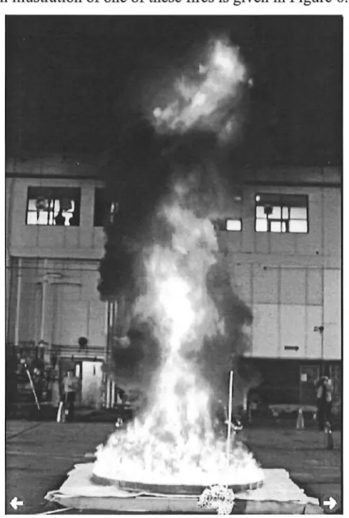
The high bay hanger experiments in Hawaii that are used in this research have been used previously to compare against predictions made by various field models. Gott et al (1997) explains how NIST-LES was used prior to the tests at the facility being performed, to obtain an idea of the size of fires that were needed in order to activate sprinklers of different activation temperatures. A quantitative comparison of the experimental data was not performed.
Davis et al (1996) used the CFD models CFX and NIST-LES as well as a number of zone models to predict temperatures in the Hawaii hanger. The geometry and dimensions of this hanger are explained in more detail in Section 6.1. Davis et al (1997) concluded that the performance of the CFD models were better than the zone models in some comparisons but very poor in others. The NIST-LES results over predicted the experimental results of the tests considered. The reason for this was thought to be due to the poor grid resolution. It was observed that the model was in good agreement with the plume temperature correlations when the grids were in the order of one tenth of the characteristic fire diameter. The NIST-LES model worked best when the fire was large enough so that the entrainment processes could be modelled directly without resorting to an empirical turbulence model. For the fire sizes used there was still some relevant mixing that was not resolved which led to the higher temperatures that were observed in the plume (Davis et al, 1996).
2.3
Fire modelling for design
indicated that the activation times and gas temperatures after the sprinkler activation fell within 20% of the experimental results (Baum, 2000).
Using field modelling for design purposes is fast becoming the norm in industry. However, care must be taken to evaluate the nature of the particular scenario and assess the ability of the field model to accurately simulate it.
2.4
Summary
Section 2.2 outlined a range of studies that have been performed to compare various field models with experimental results. Generally these models gave good far field predictions but poor predictions for areas close to the fire and in the fire plume. This was due to the grids not being small enough to adequately resolve the mixing processes in these areas. It was also apparent that most of the combustion models used in the simulations were inadequate in modelling the actual fire behaviour and fire temperatures.
Limited studies have been performed on the effect of changing grid size, which is the main topic of this research. The limited data available suggested that finer grids did produce much better predictions of centreline plume temperatures but the improvements were only small for areas further away from the fire. Davis et al (1996) observed that when the grids were in the order of one tenth of the characteristic fire diameter the model gave predictions that were in good agreement to experimental plume centreline temperatures.
3
FDS model
This chapter outlines the various concepts and equations behind the FDS model. It is only designed to give a brief overview and broad understanding of the mathematics behind the field model, the aim being to develop a familiarity with FDS.
The main references sited and are the work of Hinze (1975), who describes the equations and in-depth theory behind turbulence; McGrattan et al (2001), who provides the actual equations used in FDS and Cox (1995), who provides the derivations and basic concepts for the conservation equations and turbulence modelling.
3.1
Hydrodynamic model
The general fluid dynamic equations describing the transport of mass, momentum and energy can be used to describe a large and varied array of physical processes, many of which have nothing to do with fire. This generality is not needed in fire models and would only serve to complicate what is already a complicated task. The simplified equations, developed by Rehm and Baum (McGrattan et al, 2001) use an approximate form of the Navier-Stokes equations for flow in a thermally expandable multi-component fluid. The original Navier-Stokes equations, as well as derivations from first principles, are given in Hinze (1975, Chapter 1). This simplified form is achieved by filtering out acoustic waves to obtain what is known as the "low Mach number" equations. They describe the low speed motion of gases, driven by a chemical heat release and buoyancy forces. These equations allow for large variations in density and temperature but only small changes in pressure, which are typical of fire scenarios (Floyd et al, 2001).
3.1.1
Conservation of Mass
Generally, the conservation of mass states that the rate of mass storage, due to density changes within a control volume is balanced by the net rate of inflow of mass by convection (Lovatt, 1998). If the density is constant then the equation simply states that what flows in must flow out (Cox, 1995). The equation is written as:
dp
-+V·pu=O
dt
Equation 3.1The first term describes the density changes with time and the second defines the mass convection; u is the vector describing the velocity in the u, vand wdirections.
3.1.2
Conservation of Momentum
The equation for the conservation of momentum is derived by applying Newton's second law of motion, which states that the rate of change of momentum of a fluid element is equal to the sum of the forces acting on it (Cox, 1995):
p(
~~
+ (
u ·V)u) + V p = p g +
f+ V · r
Equation 3.2
Here the left hand side represents the rate of change of momentum of a volume of fluid, while the right hand side comprises the forces acting on it. These forces include gravity (g), an external force vector (f) (which represents the drag associated with sprinkler droplets that penetrate the control volume) and a measure of the viscous stress ( 't) acting on the fluid within the control volume. Of these three forces, gravity is the most important because it represents the influence ofbuoyancy on the flow.
turbulence in the control volume. The viscosity term is calculated depending on the mode of simulation in FDS, which in turn depends on the grid resolution. The two modes are Large Eddy Simulation (LES) and Direct Numerical Simulation (DNS) and are described in more detail in Section 3.2 below. For the LES approach to fire modelling, where the grid resolution is not fine enough to capture all the relevant mixing processes, the sub-grid analysis of Smagorinsky is 'used to model the viscosity (McGrattan et al, 2001). This also utilises the deformation tensor mentioned above to arrive at a value for the local turbulent viscosity based on the density, an empirical constant and a characteristic length (which is in the order of the grid size used in the model). This turbulent viscosity can then be used to calculate thermal conductivity and diffusivity for the LES model. The various equations used to define these tensors and variables can be found in McGrattan et al, (2001) and more rigorous derivations of the turbulence modelling in Hinze (1975) and Cox (1995). The FDS model uses a set of different equations to directly model the diffusion if the DNS mode is used. The equations for these are also described in McGrattan et al, (2001).
The equation for the conservation of momentum (Equation 3 .2) is simplified by utilising various substitutions as well as assumptions concerning the sources of vorticity in the force terms to obtain a linear algebraic equation that can be solved quickly and directly in the model calculations using fast Fourier transforms. The exact equations associated with this simplification can be found in McGrattan et al (2001).
3.1.3
Conservation of Energy
The left side describes the net rate of accumulation, while the right side is comprised of the various energy gain or loss terms that contribute to this accumulation. These include the energy driving the system, represented as the HRR ( q"'), the radiative flux ( qr) and the convective term
(VKVT).
The last term represents the energy change associated with species interdiffusion.3.1.4
Conservation of Species
The conservation of species also has to be preserved within the system. The following equation is used in FDS to achieve this:
~
at
(p Jj)+
V · p Jju=
"\? · (pD) 1 "\?Jj
+
Uj'u
Equation 3.4
The first term on the left side represents the accumulation of species due to a change in density, the second term is the inflow and outflow of species. The right side gives the terms for the inflow or outflow of species from the control volume due to diffusion and the production rate of the particular species.
3.2
Combustion model
There are two types of combustion models used in FDS. The choice of model is dependent on the grid resolution of the particular simulation. DNS is used when the diffusion of fuel and oxygen can be modelled directly (McGrattan, 2001). This applies when the grid size is very fine. For larger grid sizes, more often used in commercial applications of FDS, a LES calculation is performed.
The mixture fraction is a quantity representing the fraction of material at a given location that originated as fuel (McGrattan et al, 2001), and is defined as:
Z=
sYp-
(Yo-
J;)
Tn · f
Sip
+I;;'
Equation 3.5This equation specifies that Z varies from one in the region containing only fuel, to zero where the oxygen mass fraction equals its ambient value, Y oinf.
This mixture fraction combustion model approximates the combustion process in both space and time so that the fire can be simulated more efficiently (Floyd et al, 2001 ). It assumes that large-scale convection and radiative transport phenomena can be modelled directly while small scale mixing can be ignored (McGrattan et al, 2001). An infinite reaction rate can be assumed because the combustion processes are on a much shorter time scale than the convection processes. This means that the reaction occurs so rapidly that both fuel and oxygen cannot coexist (Ma & Quintiere, 2001). As a consequence, at a certain point both species instantaneously vanish, their mass fractions (Yi) dropping to zero. Equation 3.5 can therefore be simplified to obtain the flame mixture fraction (Zf) at which this occurs:
Equation 3.6
This point (Zf) defines the flame by prescribing a two-dimensional surface in the three-dimensional computational domain (Floyd et al, 2001) and is known as the flame sheet.
The assumption that fuel and oxygen cannot coexist can also be used to define the state relation between the oxygen mass fraction (Yo) and the mixture fraction (Z):
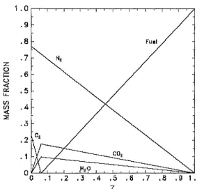
The mass fractions of all the other species of interest can also be described by individual state relations based on the mixture fraction. These state relations are determined by analysis of the stoichiometric reaction of the particular fuel in question. This is explained in more detail in Floyd et al (2001). Figure 3.1 is an illustration of the relations between the mixture fraction and the mass fraction (state relations) of various species for propane. Where the Fuel and 02 (oxygen) lines meet at a mass fraction of zero is where the flame sheet is defined, as explained above.
1 . 0
.9
.8
.7
z 0
.6 i= u
<C
a:: .5
lL VI
.4
{/)
-41.:
:.=E
.3
.2
. 1
• 1 • 2 .4 .5 .6 .7 .B .9 1.0
[image:44.602.152.435.240.511.2]z
Figure 3.1: State relations for propane (McGrattan et al, 2001).
Since the local oxygen mass fraction has been defined (Equation 3.7), its derivative with time can be used as a means of determining the oxygen consumption rate (111o'"). This is then used to calculate the local HRR by multiplying it with the HRR per unit mass of oxygen (LlH0 ).
One problem that occurs due to the local HRR calculation procedure (outlined above) is that if the fire is not adequately resolved the flame surface defined by the mixture fraction Z
= Zr
will tend to underestimate the observed flame height. An indication of whether the fire is adequately resolved is given by the ratio D* /ox. Where D* is the characteristic fire diameter defined as:
2
v~(p_c,~)gr
Equation 3.8
and ox is the nominal grid size. It has been found that a better estimate of the flame height can be provided by using a different value for the mixture fraction (Z). The expression that is used to calculate this new mixture fraction (Zr,eff) is:
Zf,etr . ( D*)
--=mm 1 , C
-Zf
ox
Equation 3.9C is an empirical constant that is independent of the scenario being simulated (McGrattan et al, 2001).
3.3
Thermal radiation model
be expected for a particular point in a diffusion flame. Because radiation is dependent on the fourth power of temperature this can have a significant impact on the calculated radiation from those particular grids. Elsewhere the temperature is calculated with greater confidence so the source term can assume its ideal value (McGrattan et al, 2001). The radiation relations become:
!db
=
K(J'T I 1CXrqm I 4tc
Outside flamezone
Inside flamezone Equation 3.10
q"' is the HRR per unit volume and
Xr
is the local fraction of that HRR emitted as thermal radiation. This is not necessarily the same as the global radiative fraction due to re-absorptionby smoke released from the fire. This is particularly the case for larger fires. K is the local
absorption coefficient and is dependent on the mixture fraction and temperature. It is determined by a sub-model implemented in FDS called RADCAL (McGrattan et al, 2001).
4
McLeans Island Tests
4.1
Experimental set-up
The McLeans Island isoroom tests were performed by the Civil Department at the University of Canterbury in November and December 2000. The tests consisted of two isorooms, which were the standard dimensions of 2.4 x 3.6 metres by 2.4 metres high. The separating wall between the two rooms was constructed of timber and was a total of 0.2 metres thick. A standard doorway connected the rooms; this was 0.8 metres wide by 2 metres high. Figure 4.1 provides an illustration of the layout and dimensions of the isorooms. One end of the second isoroom was entirely open to allow ventilation and the smoke and gases to flow freely out and into the natural draft exhaust hood above. The entire compartment including the ceiling, floor and all walls were lined with 12mm thick fire rated gypsum board overlaid with 25mm thick Fibreglass board (sold as "Intermediate service board") (Fleischmann, 2000).
)
/ /
Fire Room
/L
-/~~~'
IIIII
/ BUt'IICI'
3.6 m
800
mm
3.6 111
Adjacent Room
Ft•ont Opening
[image:47.600.85.499.430.659.2]The fire source was a LPG burner measuring 0.3 x 0.3 x 0.2 metres deep and sat 0.1 metres off the floor. The fuel flow could be controlled to generate a known HRR. A number of tests were performed using different heat outputs and burner placements. The HRRs ranged from 55 kWto 165 kW and all except one had the burner situated in the centre ofthe compartment (Fleischmann, 2000).
The tests used for comparisons in this report all had the burner at the centre of the first or rear isoroom, henceforth described as the fire room. Two experiments with HRRs of llOkW and 55kW were used for the model comparisons.
A series of nine thermocouple trees were used in the tests (see Figure 4.2). These were all placed along the centreline of the compartment. Trees #1 to #4 in the fire room were located at 0.15, 0.9, 1.8, and 2.7 metres from the rear wall. Trees #6 to #9 in the adjacent room were at 0.9, 1.8, 2.7 and 3.6 metres from the wall joining the two rooms (see Figure 4.2). On each of these trees were thirteen thermocouples at heights of 0.3, 0.6, 0.9, 1.1, 1.35, 1.6, 1.85, 2.1, 2.15, 2.2, 2.25, 2.3, 2.35 and 2.375 metres above the floor. The final tree (Doorway tree) was
\
located in the centre of the doorway with thermocouples at 0.1, 0.25, 0.4, 0.55, 0.7, 0.85, 1.0, 1.15, 1.3, 1.45, 1.6, 1.75 and 1.9 metres above the floor. (Fleischmann, 2000).
Fire Room Front Room
Tree #1 Tree tf2 Tree #J Tree #4 Doorway tree Tree #6 Tree #0 Tree #1
+ +
Burner+ + + + +
3.7m
0.15m* 0.9m 1.8m 2.7m 4.6m 5.5m 6.4m
'Distance from rear wall
16 species concentration probes were also placed along the centre of the compartments; a set of four in each of the locations corresponding to trees #2, #4 and #7 (see Figure 4.2) at heights of 0.3, 0.6, 1.95 and 2.25 metres, and a set of four in the doorway (Doorway tree) at heights of 0.4, 0.7, 1.6 and 1.9 metres (Fleischmann, 2000).
4.2
FDS modelling
4.2.1
Grid sizes
Models with a grid size of lOOmm, 150mm and 300mm were constructed. These correspond to enclosure height over grid size ratios ofH/24, H/16 and H/8. These sizes were based on the physical dimensions of the burner. This meant that the burner or more specifically the HRR was being characterised more precisely.
For each grid size two fire sizes were modelled: 55kW and llOkW. The output from the FDS model is not exact in regards the HRR so in order to obtain the required HRR several runs had to be performed, each time changing the HRRPUA specified in the input FDS file until the required output HRR was obtained. Table 4.1 gives the final HRRPUA used for each model and the corresponding output HRR obtained.
Table
4.1:
Input HRRPUA and output HRRs for the McLeans IslandFDS
models.11 OkW experiment 55kW experiment
Grid size HRRPUA HRR Error HRRPUA HRR Error
100 mm (H/24) 1387 108 -1.8% 770 54 -1.8%
150 mm (H/16) 1305 111 0.9% 750 55 0%
300 mm (H/8) 1 035 109 -0.9% 554 55 0%
4.2.2
Model discrepancies
FDS models sometimes could not be placed exactly in the centre of the room. This was the case for the models with the lOOmm and 300rnrn grids. Also the thickness of the connecting wall could not be modelled exactly for the 150rnrn and 300mm grid size models because the actual thickness was 200mm. The dimensions of the door between the two rooms also became a problem, especially for the two larger grid sizes. Appendix A, Table A.1 gives a detailed list of the differences between the experiments and the FDS models used.
4.2.3
Input variables
All the surfaces in the isorooms were lined with a 12rnrn thick layer of fire rated gypsum board overlaid with a 25rnrn thick layer ofFibreglass board (Fleischmann, 2000). Because the FDS code only allows for one material in the heat transfer calculations (without a lot of added complexity) it was assumed that the top fibreglass layer was the dominant material contributing to the heat transfer out of the compartment. This fibre glass layer was the thicker of the two and had the greatest thermal resistance. The layer was modelled as thermally thick, which specifies the model to perform a one dimensional heat transfer calculation though the surfaces (McGrattan et al, 2001). The properties required for the thermally thick calculation were the thermal diffusivity (ALPHA), 8.6 x 10⁻⁸ m2/s (Quintiere, 1998) and the thermal conductivity (KS), 0.036 W/m.K (Incropera & DeWitt, 1996). These are also tabulated in Appendix D. The terms in brackets (following the variable name) are the call names that are used in the actual FDS input files. These input files are given in Appendix B.l. The thermal properties were based on data for fibreglass board found in the various references cited. It is uncertain, due to lack of relevant documentation whether it is equivalent to what was used in the actual experiments. However, these values do not have to be exact as long as they provide a close approximation to the experiments. The nature of the comparisons between different grid sizes will be enough to deduce the required trends and establish relevant conclusions.
4.3
Zone modelling
The zone model CF AST was also used to give comparisons against the FDS models. The isorooms were simply modelled as two rooms of 2.4 x 3.6 metres by 2.4 metres high, connected by a vent or door measuring 0.8 by 2 metres. The front isoroom (Figure 4.2) was assigned an opening of 2.4 by 2.4 metres; this sirimlated the wall opening that was used in the experiments. The burner was located at the centre of the fire room and assigned a HRR depending on the test being simulated, either llOkW or 55kW. The walls, floor and roof were manually assigned thermal properties. These were equivalent to the thermal properties used in the FDS model as described in Section 4.2.3 for fibreglass board. All the properties are given in Appendix D, Table D.2. The zone model was set to simulate 3600 seconds of fire time.
4.4
Data analysis
As a result of the large amount of data that was obtained from the FDS models and the experiments, some form of data reduction had to be used so that it could be compacted and presented in a more manageable form. This section serves to outline the various techniques that were used to achieve this.
4.4.1
Temperature measurements
The average temperature of each thermocouple was calculated for the steady state period of the experiment. This was assumed to start at 1000 seconds and continue to the end of the test (3600 seconds). The initial 1000 seconds allowed to reach steady state was a conservative start up time based on observation of the time-temperature profiles of the experimental results. The FDS model temperature predictions were also averaged over the same time period.
4.4.2
Layer height
In order to compare FDS and experimental results with predictions made by the zone model, CFAST, an indication oflayer height was required. To do this the temperature gradients were calculated between each pair of adjacent thermocouples. The layer interface was assumed to occur half way between the two thermocouples which gave the greatest temperature gradient. This was assumed to be analogous to where the cool lower layer meets the hot upper layer in the more simplified zone model predictions. The layer height was calculated for each thermocouple tree and an average taken to obtain one layer height for each of the two isorooms. The tree above the burner (tree #3) was not used in this calculation because a marked temperature difference does not occur in the fire plume. The doorway tree was also excluded from the layer height calculations because it is not indicative of the room layer heights.
4.4.3
Upper and lower layer temperatures
Comparisons were also made between upper and lower layer temperatures. A weighted average of the thermocouple readings was calculated based on the distances between each thermocouple and the layer height (as calculated in Section 4.4.2). This was done for each thermocouple tree and averages taken for each isoroom. Tree #3 and the doorway tree were again not included in the layer temperature calculations.
4.4.4
Oxygen concentration data
5
McLeans Island Results
This section presents the results from the FDS simulations of the McLeans Island isoroom tests. FDS models using three different grid cell sizes were used in the comparisons: lOOmm (H/24), 150mm (H/16) and 300mm (H/8). Two sets of results are compared; the 55kW test and the llOkW test. Each set of comparisons include:
• Comparisons of thermocouple tree temperature profiles generated from the measurements taken in the experiments and those predicted by the FDS models.
• Comparisons of layer heights obtained from the experimental data, FDS model predictions and zone model results.
• Comparisons of upper and lower layer temperatures obtained from the experimental data, FDS model predictions and zone model results.
• Comparisons of experimental and FDS model oxygen concentrations at particular points in the isorooms.
5.1
55kW test
5.1.1
Temperature tree profiles
]:
...
~
~ 1.0 1
-0.5
---- ---- ---- 1 OOmm grids ···--·-···--·-·--·-···-···- ···- --150mm grids __ _
- - 300mm grids • Experimental
0.0+---,----~~~-~---~.-~--.----,---,---.---~
0 20 40 60 80 100 120 140 160 180
Temperature
eq
Figure 5.1: Temperature profiles for Tree 1 for the 55kW fire.
2 . 0 1
-1.5
•----1
-···-···-·--···- ... ····-·-··- _ .. ..'!L ...
·-·-·--·--··----·----·-···----·-···-·---;
..
\
\.~1111--t
- - - lOOmm grids --150mm grids - - 300mm grids • Experimental
0.0+---~---,----.---.---,---,----,----~
0 100 200 300 400 500 600 700 800
Temperature (0C)
Figure 5.2: Temperature profile for Tree 3 (directly above the burner) for the 55kW