Simulating Coupled Longitudinal, Pitch and Bounce Dynamics of Trucks with Flexible Frames

Simulating Coupled Longitudinal, Pitch and Bounce

Dynamics of Trucks with Flexible Frames

D. Geoff Rideout

Faculty of Engineering and Applied Science, Memorial University, St. John’s, Canada Email: g.rideout@mun.ca

Received August 7,2012; revised September 8, 2012; accepted September 19,2012

ABSTRACT

Simulating the dynamic response of trucks requires that a model be constructed and subjected to road inputs. Inclusion or omission of flexible frame effects is often based on intuition or assumption. If frame vibration is assumed to be sig-nificant, it is typically incorporated in one of two ways. Either a complex finite element model of the frame is used, or a simplified linear modal expansion model (which assumes small motions) is employed. The typical low-order modal expansion model, while computationally efficient and easier to use, is limited by the fact that 1) large rigid body mo-tions and road grade changes are not supported, and 2) longitudinal dynamics are not coupled to vertical and bounce dynamics. In this paper, a bond graph model is presented which includes coupled pitch and bounce motions, longitudi-nal dynamics, and transverse frame vibration. Large rigid body motions are allowed, onto which small flexible vibra-tions are superimposed. Frame flexibility is incorporated using modal expansion of a free-free beam. The model allows for a complete pitch-plane representation in which motive forces can propel the truck forward over varying terrain, in-cluding hills. The effect of frame flexibility on vehicle dynamics can then be studied. This is an extension of the typical half-car model in which suspension motion is assumed vertical, pitch angles are small, and longitudinal dynamics are completely decoupled or omitted. Model output shows the effect of frame flexibility on vehicle responses such as for-ward velocity, pitch angle, and payload acceleration. Participation of individual modes can be seen to increase as road input approaches their natural frequency. The bond graph formalism allows for any or all flexible frame modes to be easily removed from the model if their effects are negligible, and for inclusion of more complex submodels for compo-nents such as suspension and engine if desired.

Keywords: Truck Model; Vehicle Dynamics; Pitch Plane; Frame Flexibility; Bond Graphs

1. Introduction

The dynamic analysis of trucks requires a mathematical model of the vehicle structure (including engine, cab, and transmission), suspensions and tires, and the road excita-tion. While flexural vibration of the chassis can often be neglected in smaller, relatively stiff automobiles, large trucks and buses can experience significant “beaming mode” vibration. Beaming is response of the frame at its first modal transverse bending frequency, and for non- articulated trucks this frequency can be on the order of bounce and pitch frequencies of a rigid vehicle [1-3]. Beaming response can be sizeable at the centre of the frame midway between the steered wheels and rear axle [4].

Approaches to modeling flexible vehicles range from 1) ignoring body flexibility by using a lumped mass model [5]; 2) modeling the frame as a regular free-free beam and calculating, estimating or measuring modal masses and stiffnesses [4,6]; and 3) modeling the entire vehicle

the vehicle encounters bumps, and therefore when sus- pension and body motions in the pitch plane are excited. Vertical road undulations and the resulting pitch plane response can also affect longitudinal motion. In other words, for certain vehicle parameters and road roughness, there can be two-way coupling between longitudinal and pitch/bounce motion [11-13]. To maximize the accuracy of vehicle response prediction when such coupling is present, and to further account for the effect of frame flexibility, the typical small-vertical-motion model with frame vibration must be extended to allow the large rigid body motions that arise from longitudinal motion and change in road inclination.

This paper presents a model which includes pitch and bounce motions, longitudinal dynamics, and transverse frame vibration. Forces and velocities are resolved along coordinate axes parallel and perpendicular to the unde- formed frame. Large rigid body motions are allowed, onto which small flexible vibrations are superimposed. Frame flexibility is incorporated using modal expansion of a free-free beam. The model allows for complete pitch-plane representation in which motive forces can propel the truck forward over varying terrain, including hills. The effect of frame flexibility on vehicle dynamics can then be studied. The bond graph formalism is used to generate the model. Bond graphs, in addition to facilitat-ing integration of flexible and rigid subsystems, allow for inclusion of more complex submodels for components such as suspension and engine if desired.

The following section reviews pitch plane models and approaches to including flexibility effects. Section 3 pro- vides an overview of the bond graph modeling language. Section 4 gives schematics and equations for the rigid and flexible portions of the vehicle model, describes how terrain undulations are incorporated, and presents the final bond graph. Section 5 contains model output, in- cluding a study of the effect of road roughness on the coupling between frame flexibility, vehicle response in the pitch plane, and longitudinal motion. Discussion, conclusions and future work comprise Section 6.

2. Literature Review

Traditionally, linear pitch plane models have been the starting point for low-order modeling of truck dynamics including frame flexibility. Margolis and Edeal [4] cre- ated a 2 degree-of-freedom, small vertical motion bus frame model to which the engine, cab, and load were added in addition to suspension forces. The bond graph approach facilitated addition of external components to the flexible substructure. Frequency response of the frame showed a dominant beaming mode at approxi- mately 10 Hz, very near the unsprung mass frequency. Margolis and Edeal [5] extended the aforementioned

model to a five-axle tractor-trailer with submodels for engine, cab, and sleeper module/fuel tank. Non-linear elements were included in the model. Dynamic motions, in which the relative velocity across the suspension re- mained nearly zero, were identified as a significant effect of interaction between vehicle dynamics and frame vi-bration.

Michelberger et al. [14] identified a discrete transfer function for a free-free beam model of a two-axis bus, and then estimated modal characteristics based on meas- ured data. For an air suspension bus, frequencies of 6.7 and 12 Hz were associated with the first two bending modes of the frame. Interaction of frame motion with the other vehicle dynamic elements is foreseeable given the 9.1 Hz engine mount natural frequencies and 10.3 - 10.4 Hz wheel-hop frequencies of the front and rear axles. Ibrahim et al. [9] modeled a truck frame using modal superposition, with modal properties calculated using a finite element model. The linear model included truck longitudinal velocity and a cab suspended by two linear suspension systems. The model assumed constant longi- tudinal velocity and no aerodynamic effects or tire lift-off. Frame flexibility was found to strongly affect driver’s vertical acceleration and cab’s pitch acceleration for a truck with frame natural frequencies of 7.25, 13, and 18 Hz. Yi [15] generated a 20-node finite element model of a frame modeled as a block, with both vertical and lateral vibration degrees of freedom. Response of rigid vs. flexible models to a pulse steering input showed significant discrepancies in predictions of lateral motion and tire deformation. Cao [16] developed a modal su- perposition representation of a truck frame rail with five segments—a front rail, kick-down rail, mid rail, kick-up rail, and rear tail. The frame rails were assumed to be the primary contributors to beaming mode. In the model 312 Nastran elements were used. The frame was modeled in isolation rather than as part of a vehicle model, without considering the effects of engine, cab, box and cab mounts that were acknowledged to affect the beaming frequency and nodes.

dom model with three rigid transverse beams joined by two massless flexible beams. The flexible beams have torsional and transverse compliance. Measured data and the influence coefficient method were used to populate the mass, stiffness, and damping matrices of a linear model. Flexibility was found to have a significant effect on pitch and roll angle predictions for a bus. While dis- cretized bending representations are easy to implement and offer more insight into vehicle response than a rigid frame, a large number of elements are typically required to give a very close approximation of the lowest natural frequencies. Modal expansion has the advantage of giv- ing the correct natural frequencies of the first n modes that are retained. Given the uncertainties in determining natural frequencies analytically for a complex irregular beam with multiple attachment points, either a discre- tized or modal expansion model can be tuned to match measured natural frequencies in practical applications.

The previously cited works show a range of modeling complexities in accounting for flexibility of heavy truck frames, and verify the potential importance of that vibra- tion in vehicle dynamics models. However, prior models assume small angular motions of the frame, and do not include longitudinal dynamics along with pitch and bounce dynamics. As stated in the introduction, this pa- per combines longitudinal, rigid pitch and bounce, and transverse flexural dynamics of a truck into a single, computationally efficient model implemented using the bond graph graphical modeling language. Background on bond graphs follows, after which the model details are presented.

3. Bond Graph Modeling Language

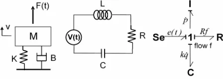
In bond graphs, generalized inertias and capacitances store energy as a function of the system state variables (momentum and displacement, respectively), sources provide inputs from the environment, and generalized resistors remove energy from the system. The time de- rivatives of generalized momentum p and displacement q are generalized effort e and flow f. Power is the product of effort and flow. For example, force and voltage are efforts, velocity and current are flows, linear momentum and flux linkage are generalized momenta, and transla- tional displacement and charge are generalized displace- ment variables.

Power-conserving elements allow changes of state to take place. Such elements include power-continuous generalized transformer (TF) and gyrator (GY) elements that algebraically relate elements of the effort and flow vectors into and out of the element. In certain cases, such as large motion of rigid bodies in which coordinate transformations are functions of the geometric state, the constitutive laws of these power-conserving elements can

be state-modulated. Generalized series and parallel con- nections are represented by 1 and 0 junctions. All ele- ments bonded to a 1-junction have common flow, and their efforts sum algebraically to zero. All elements bonded to a 0-junction have common effort, and all flows algebraically sum to zero. Sources represent ports through which the system interacts with its environment. See for example Figure 1 where the effort source repre-

sents either the force source or battery, and generalized flow associated with the 1-junction is either velocity or current.

The power conserving bond graph elements—TF, GY, 1-junctions, 0-junctions, and the bonds that connect them —are collectively referred to as “junction structure”.

Figure 2 defines the symbols and constitutive laws of

sources, storage and dissipative elements, and power- conserving elements in scalar form. Bond graphs may also be constructed with the constitutive laws and junc- tion structure in matrix-vector form, in which case the bond is indicated by a double-line. Power bonds contain a half-arrow that indicates the direction of algebraically positive power flow, and a causal stroke normal to the bond that indicates whether the effort or flow variable is the input or output from the constitutive law of the con- nected elements. See Figure 3 where the effect of causal

stroke location on the constitutive law form of two ge- neric elements A and B is illustrated.

The constitutive laws in Figure 2 are consistent with

the placement of the causal strokes. Full arrows are re- served for modulating signals that represent powerless information flow such as orientation angles that deter-mine the transformation matrix between a body-fixed and inertial reference frame. Bond graphs, because they use the same small set of symbols for energy storage, dissi- pate and exchange in any energy domain (electrical, me- chanical, hydraulic, etc.), the assembly of submodels from various disciplines is straightforward. For example, connecting a motor model to a linkage model requires simply “bonding” the 1-junction for motor output rota- tional speed to the 1-junction for linkage input link rota- tional speed.

Causality (equation input-output structure) automati- cally propagates through the entire model upon assembly of submodels. The graphical representation of causality

Figure 2. Bond graph symbols.

       

1 1

e f

A B

e f

A B

f e e f

e  f f 

    

    

A B

A B e

Figure 3. Bond graph causality.

allows for visual detection of input-output conflicts be- tween subsystems, and immediately indicates any nu- merical simulation issues such as algebraic loops or dif- ferential-algebraic equations. The reader is supposed to refer to [18] for more details on bond graph modeling.

The truck model is implemented using bond graphs in

this paper, and uses 20 sim [19] commercial software to enter the graph, generate and simulate equations of mo- tion, and plot results. The implementation could be done (albeit with more tedious equation derivation) in software such as Matlab.

4. Vehicle Model

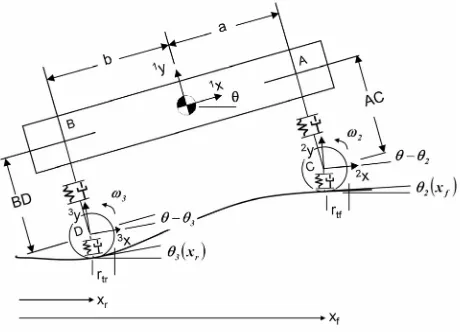
Figure 4 shows a schematic of the pitch plane vehicle

model. The rigid aspects of the model are based on [20] and [13]. The model permits large angular motions of the sprung mass and uses nonlinear constitutive laws for aerodynamic drag and tire slip and rolling resistance. The aerodynamic drag constitutive law assumes that drag coefficient and frontal area are constant, and the effect of crosswinds is not considered. After the rigid model as- pects are reviewed, the superposition of transverse beam vibrations onto the motion of the rigid frame will be de- scribed.

4.1. Rigid Body Dynamic Elements

Referring to Figure 4, suspension mounting points are A

and B, with unsprung masses at C and D. The unsprung masses are constrained to move along lines AC and BD perpendicular to the undeflected frame. Rotating coordi- nate frames 1, 2, 3, and 4 are affixed to the frame, cab/ engine, road at front contact patch, and road at rear con- tact patch respectively. The cab and engine mount to the frame at points M and N via stiff “parasitic” springs with damping, which model bushings [21]. The load is mod- eled as a point load at L, also connected to the frame with a parasitic spring/damper. The load is assumed to provide no stiffening effect on the frame. If a physical prototype exists, then a modal test of the laden frame could be done to reveal natural frequencies and mode shapes for use in the flexible model in the next section. The parasitic spring/damper connection method preserves an explicit ordinary differential equation structure by breaking the

dependency among the load, cab/engine, and frame rigid body momenta. Having coordinate frames with the x axis aligned with the road at each tire facilitates inclusion of longitudinal tire slip (traction) and rolling resistance forces, which are applied in the 3_{x and} 4_{x directions.}

Tire stiffness and damping forces are always normal to the road surface as the ktsprings and bt dampers are con-

strained to deflect along the 3_{y and} 4_{y axes.}

In lieu of a road height velocity profile, the road is in- put to the model as a slope (the arctangent of which is the road inclination angle θ2 or θ3), that varies as a function

of distance xf or xr traveled by the front or rear of the

vehicle. Front and rear wheel hub forward velocities are integrated, with the resulting displacements serving as inputs to road slope look-up tables.

The traction force is a nonlinear function of wheel slip and normal load [20]. Parameters were estimated from measured data of an actual Class VI truck tire. The slip resistance arises due to tire compliance and the resulting difference that can occur between the actual forward ve- locity v of a wheel hub and the velocity if the tires were rigid, i.e. tire radius r multiplied by wheel angular ve- locity ω. Defining slip ratio  as

r v v



   (1)

the slip resistance force is

 

slip

max

sgn F_z

F   



 (2)

where Fz = tire force normal to the road,  = coefficient

of friction, max = slip ratio at tire saturation, and “sgn” is

the signum function, which returns the algebraic sign of its argument. Rolling resistance is also a function of normal load Fz and longitudinal velocity, along with tire

inflation pressure P and empirical constants ci.

 

rolling sgn 1 2 z 3 z 4 z

F  v c_ c F c F P c F P_ (3) The aerodynamic drag constitutive law is given below. The drag force is proportional to the body-fixed x-com- ponent of the sprung mass longitudinal velocity. The drag coefficient is thus held constant regardless of changes in the pitch attitude of the vehicle.

1 1

aero 0.5 d Cx Cx

F  AC v v (4) where  = air density [kg/m3_{], A = frontal area [m}2_{], C}

d =

drag coefficient (dimensionless), 1_v

Ox = longitudinal ve-

locity [m/s]. A complete set of vehicle parameters is given in Section 5.

4.2. Flexible Substructure

The transverse deflection of the frame is given by



flexibility modeling is based on the well-known partial differential equation for transverse vibration



w x t

 

w x t of a free-free beam of length L:









4 2

1 1 2

4 2 δ

w w

EI A F x x F x

x  t

 _  _{  }

 



(5)

with zero bending moment and shear force boundary conditions. Inputs to the beam due to suspension, cab, or payload mounting points are modeled as point loads mul- tiplied by the Dirac delta function at the location of the point, as shown on the right-hand side of Equation (5).

Referring to Figure 4, the coordinate frame 1x −1y ro-

tates and translates with the undeflected “shadow” frame of the vehicle, and deflections are assumed relative to the shadow frame in the 1_{y direction. The}

frame flexure in the 1_{y direction follows the free-free}

beam derivation of [18] and [22] in which the decoupled modes include rigid body translation and rotation. Rigid body translation occurs along the 1_{y axis, the orientation}

of which can change with road slope. Rigid body rotation angle is the angle of the 1_{x axis with respect to the iner-}

tial 0_{x axis. This angle will change with road slope.}

Separation of variables gives the solution as an infinite sum of the product of spatial functions (mode shapes)



w x t

 

n

W x and time functions 

 



 

   

1

, n

n

w x t W x  t







Substituting Equation (6) into (5), multiplying by or- thogonal mode shapes and integrating over the beam length gives an infinite set of uncoupled modal dis- placement equations of motion for a system with external forces acting at two points 1 and 2:

 



1 1 2

n n n n n n

m k FW x F W x2



by 2 0 d L n

m 



n

(8)

2 n n

k m (9) Parameter values for the flexible subsystem are listed in Section 5. Three bending mode natural frequencies are included, with natural frequencies 11.7, 32.4, and 105 Hz. The parameters correspond to a truck frame made from four parallel 10 × 20 cm steel box sections with 2.8 cm thickness.

Superposition of the small flexural displacements

 

w x t , in the 1_{y direction, onto the gross motion of the}

undeflected frame as described above implies the fol- lowing assumptions:

transverse bending modes, for which frequencies are not high enough to warrant treatment of the frame as a Timoshenko beam

 rigid body and flexible motions are decoupled. The flexibility of a truck frame and the angular velocity of its rigid body motion, are not assumed large enough to cause inaccuracies due to changes in beam length [23], or geometric stiffening [24].

When low-order flexible frame modeling is limited to small motions, and no longitudinal dynamics are consid- ered, the rigid body modes can be represented as follows:

 Mode 00 (rigid body translation): mass mG moving

with linear velocity vGy in the inertial 0y direction only

 Mode 0 (rigid body rotation): inertia JG rotating with

angular velocity 1 about a fixed-orientation z axis Consider now the total velocity of point A, which is

 



1 1

1 ,

Ay Gy A

v  v  AG  w x t_





(10)

with the w term given by differentiation of Equa- tion (6). A suspension input force to the frame at point A would accelerate the frame centre of gravity G in the vertical direction, would create a moment about G to angularly accelerate the frame in the θ1 direction, and

would excite each flexible mode through a “lever arm” which equals to the modal amplitude at point A as seen on the right-hand side of Equation (7). Observing the duality between the point A velocity equation above, and a force at A propagating through rigid body and flexible modes, we can draw the following bond graph, Figure 5.



The suspension force FA, applied in Figure 5 through

an effort (force) source, would come from a suspension spring and damper in parallel. The 1-junctions (velocity nodes) represent the velocities of modes 00 through 2. Thus, two of the many infinitely flexible modes are re- tained. Rigid body mass and inertia are bonded to the rigid body modal velocity nodes. Bonded to the flexible modal velocity nodes are the modal mass, stiffness and damping. The flexible modes are thus decoupled mass-

Figure 5. Vertical dynamics beam model.

spring-damper oscillators with governing Equation (7), each of which has the appropriate modal natural fre- quency. The 0-junction (force node) for which each bond has the same effort (force) FA, directs that force through

transformer elements for which the moduli are the mode shapes at the location of point A. As the transformers are power-conserving elements that relate effort to effort and flow to flow, they also multiply the modal velocities by the mode shape magnitude. The transformed modal ve- locities are summed at the 0-junction, resulting in the total vertical velocity w x t





tion thus performs the summation of velocity terms that appears when Equation (6) is differentiated.

4.3. Extension to Include Longitudinal Dynamics The Newton-Euler approach is used to model the multi- body system. Joints are modeled by computing absolute velocities of points on different bodies, and constraining certain degrees of freedom. The absolute velocity vectors are resolved into components along the rotating body- fixed axes depicted in Figure 4. This results in gyrational

coupling terms in which forces or torques in each coor- dinate direction arise due to velocity in another coordi- nate direction. Consider for example the undeflected frame, to which coordinate frame 1 is attached in Figure 4. Equating resultant forces to the rate of change of linear

momentum gives:



1 d

dt m

  1



F v (11)

1

1 1

1

1

x x y

y y x

F mv m v

F mv m v

          _  _                      

  (12) For planar motion, rotational dynamics occur about a single axis, so that



d d

G G

M J

t 



   (13)

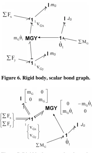
Equation (12) can be represented by the bond graph of

Figures 6 and 7, in which the force summations are rep-

resented by 1-junctions to which are bonded applied forces, inertial elements to model the first terms on the right-hand side, and a gyrator (relating effort to flow) to model the final terms. External moments and inertia are applied to a rotational 1-junction, a signal from which modulates the gyrator. Figure 6 shows a scalar bond

graph (note the separate mass elements for each coordi- nate direction), and Figure 7 is the vector bond graph

equivalent (with diagonal mass matrix and skew-sym- metric gyrator matrix). Scalar and vector bond graphs will be shown in later figures as the complete model is presented.

Incorporating the longitudinal (x) degree of freedom in

Figure 6. Rigid body, scalar bond graph.

Figure 7. Rigid body, vector bond graph.

Figure 5 gives the partial Frame submodel bond graph

of Figure 8. Because the frame centre G and the payload

point L are very close together, they are assumed to have the same 1_{x velocity. The associated I element parameter}

is thus mG + mL. The Se elements resolve the gravity vec-

tor along the 1_{x −} 1_{y axes. The power port at the rear}

suspension mounting point B is shown, at which the in- put effort Fr is the combined suspension spring and

damper force, and the flow is the 1_{y component of veloc-}

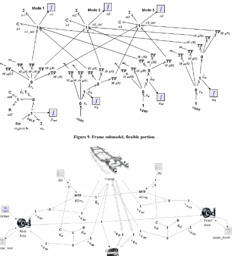
ity of B. This port is joined to the flexible modes with TF elements whose moduli are the mode shape functions evaluated at point B. Figure 9 shows three flexible

modes, defines the velocity/force port at the load location L, shows the load mass, defines the front suspension connection point A, and defines the cab mounting points M and N. Connection point B would be similar, but is omitted for clarity. The load mass mL is joined to the

frame with a parasitic spring and damper.

4.4. Suspension, Axles and Tires

Figure 10 is the top level bond graph model showing the

suspension system and submodels for Cab/Engine, Front Axle, and Rear Axle.

Referring to Figure 4, suspension spring/damper ve-

locities are the difference between the velocities of A and C (front) and B and D (rear) along the 1_{y axis. The F}

susp

0-junctions subtract the velocities, direct them as inputs to the Ks− Rs suspension spring/damper units, and direct

the suspension forces equally and oppositely to points C and D. The forward motion of the wheels and axles is

Figure 8. Frame submodel, rigid body portion.

defined using the relative velocity of C and D with re- spect to A and B in the 1_{x direction.}









1 1

1

1 1

1

Cx Ax f

Dx Bx r

v v AC y

v v BD y

       



 (14)

where hf and hr are distances between points A and C,

and B and D respectively when the suspension is unde- flected. yfand yr are front and rear suspension deflections.

Modulated transformer (MTF) elements multiply the angular velocity by the moment arm, and the Fx 0-junc- tions sum the velocity terms in Equation (14).

Velocities of points B, L, M, A and N along the unde- flected frame are assumed to have equal velocity com- ponents in the 1_{x direction. Following [25], the road pro-}

file is represented as a slope which varies as a function of distance travelled. The “slope_front” and “slope_rear” lookup tables in the top level model accept distance trav- elled by the axles as an input, and return road slope to the axle submodel tire dynamics. This allows calculation of the road profile angle (arctangent of the road slope), which defines the angles θ3 and θ4 of the coordinate

frames at the wheels. Rolling and slip resistance forces act along the road x directions, and tire stiffness forces act in the local y directions. Tire stiffness thus always acts perpendicular to the road surface, even when the surface is at an angle, while rolling and slip resistance are tangential to the road. Bumps will compress or relax the suspension and also oppose the vehicle’s forward mo- tion.

Figure 11 shows the “RearAxle” submodel, which is

Figure 9. Frame submodel, flexible portion.

Figure 10. Top-level bond graph.

I elements are included for wheel inertia and unsprung mass. The MTF elements represent the following coor- dinate transformation between road and suspension coor- dinates:

Rolling and slip resistances are clearly indicated, and each is a function of tire normal force Fzr from the

0-junction defining the tire deflection velocity.

















4

1 4 1 4

cos sin

sin cos

1

D D

       

    

  _{ }



v _

 v (15)

Figure 12 is an expansion of the Cab/Engine sub-

Figure 11. Rear axle submodel.

Figure 12. Cab/engine submodel.

bonded to the 2_v

E 1-junction. Velocities of points M and

N in frame 2 are calculated using 2_v

E and relative veloci-

ties 2_v

M/E and 2vN/E. The relative velocities are computed

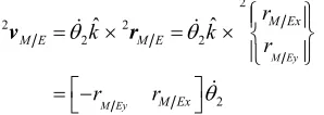
in the vector bond graph by multiplying the angular ve- locity by a subset of the skew-symmetric matrix for the position vector cross product. The product is realized in the bond graph with the TF elements.

2

2 2

2 2

2

ˆ ˆ

M Ey

M Ey

M Ex

M E M E

M Ex

r

k k

r

r r

 



 

 

   _{ } 



 

 _{ }

 



v r

 (22)

Velocities of M and N from the Frame model are in- puts to the Cab/Engine, where they are transformed to frame 2 components with rotation matrix transformers.

5. Model Output

Table 1 lists vehicle model parameters. The model is

Table 1. Vehicle parameters.

Parameter Value

Vehicle length, payload location 10 m, 5 m

Frame mass mG, inertia JG 4250 kg, 24,000 kg-m2

Cab/Engine mass mE, inertia JE 2000 kg, 2000 kg-m2

Suspension stiffness Ksf, Ksr 375 kN/m, 870 kN/m

Suspension damping bsf, bsr 31,895 Ns/m, 33,884 Ns/m

Tire stiffness Ktf, Ktr 2800 kN/m, 5400 kN/m

Tire damping btf, btr 1500 Ns/m, 2000 Ns/m

Bushing stiffnesses Ks 100 MN/m

Bushing damping bs 1 MNs/m

Unsprung mass musf, musr 500 kg, 700 kg

Cab mounting locations (OM, ON) 8.75, 9.75 m

Position of cab point M w.r.t. E (−0.5, −1) m

Position of cab point N w.r.t. E (0.5, −1) m

Undeflected suspension lengths

(AC, BD) 0.6, 0.6 m

Aerodynamic drag coefficient Cd 0.8

Frontal area A 5.2 m2 Wheel radius rwheel 0.413 m Tire inflation pressure P 115 psi

Number of tires (front/rear) 2/4

Tire friction coefficient μ 0.7

Tire slip at saturation κ 0.3

Front tire rolling resistance

coefficients (c1f−c4f) −197.4, 0.454, 18.7, −0.00244

Front tire rolling resistance

coefficients (c1r−c4r) −394.7, 0.907, 37.4, −0.00488

Wheel inertia (front, rear) Jwheelf, Jwheelr 10, 18.755 kg-m2

demonstrated first on a smooth road, beginning from rest and with zero initial conditions for all springs. A 10% slope is encountered when the vehicle has travelled 1500 m, and the road flattens again at 2000 m. A PI controller, as shown in Figure 13, is added to the RearAxle sub-

model to control forward velocity. This simulated cruise controller has a proportional gain of 1000 and an integral time constant of 10 seconds. These parameters allow some overshoot. The error is the difference between the actual vehicle speed and a setpoint of 20 m/s (72 km/h). A signal limiter restricts drive and braking torque to a maximum absolute value of 5000 N-m.

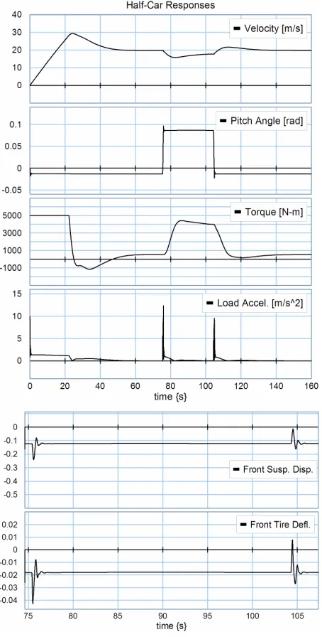
Figure 14 shows vehicle responses with a payload of

Figure 13. Vehicle speed controller.

Figure 14. Vehicle responses, smooth road

quickly to a static equilibrium value of −0.75 degrees (truck very slightly tilted forward).

When the forward velocity overshoots the setpoint, the brakes are applied and the cab tilts forward slightly more during the deceleration. After the drive torque and for- ward speed reach a steady state, the grade change is en- countered. This causes sharp transients in pitch angle and in absolute value of the total acceleration of the payload. Forward velocity momentarily drops, in response to which drive torque is increased. Pitch angle undergoes a steady state change, which is approximately equal to the road slope. Further transients, most notably in payload acceleration, occur when the road flattens out. The front suspension and tire are loaded at the beginning of the slope and unloaded at the end. Simulations are performed with 20sim bond graph commercial software, using its Backward Differentiation Formula with integration tol- erances of 1e−5.

Next, the model will be subjected to a simulated rough road, where differences between response of a flexible and rigid-frame vehicle will become apparent. Road bump spacing will be adjusted so that the frequency at which bumps are encountered is near a rigid body natural frequency, near the first (beaming) flexible natural fre- quency, and near the second flexible natural frequency. The necessity of including flexible modes in the model cannot typically be judged a priori. The rigid-element natural frequencies (e.g. ride natural frequency, wheel hop frequency) interact with the flexural natural frequen- cies of the free-free beam representing the frame. The first flexural (beaming) mode frequency will decrease with payload mass if the payload is modeled as a point mass. However, a large load anchored to the truck bed could stiffen it significantly. A model such as the one herein, where flexible modes can be added or removed and their parameters changed very easily, allows the analyst to start from a complete model and remove modes as necessary until the simplest possible model with sufficient accuracy is achieved.

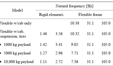
A natural frequency summary is given in Table 2. The

parasitic springs generate high natural frequencies which are decoupled from the system modes and therefore do not change with payload. These frequencies are at least an order of magnitude higher than the system modes, and are not listed in the table.

Comparison of Flexible and Rigid Models

A rough road is simulated as a series of half-sinusoidal bumps, 5 cm high and 20 cm long, repeated every 5 m. This corresponds to an input excitation frequency of 4 Hz, or 25.1 rad/s, at a vehicle speed of 20 m/s. Payload is 5000 kg. Figure 15 shows six vehicle responses for both

Figure 15. Model responses, 5000 kg payload.

Table 2. Natural frequencies.

Natural frequency [Hz] Model

Rigid elements Flexible frame

Flexible w/cab only 10.38 31.1 105.0

Flexible w/cab,

suspension, tires 1.46 3.56 10.32 31.1 105.0

 1000 kg payload 1.42 3.41 9.05 31.1 105.0

 5000 kg payload 1.27 2.96 7.71 31.1 105.0

 10,000 kg payload 1.11 2.72 7.36 31.1 105.0

tion, and front tire deflection. The vehicle speed tran- sients for an individual bump are nearly identical for both models. The pitch angle for the flexible model shows an approximately 9 Hz dynamic that is not captured by the rigid model.

Both models predict the same longitudinal payload acceleration peaks; however, the transverse (y-direction) payload acceleration is predicted poorly with a rigid model. The rigid model, without the filtering effect of a flexible beam that essentially “cradles” the load when bumps are encountered, overpredicts peak acceleration. Front suspension and tire deflection predictions are rela- tively insensitive to the inclusion of frame flexibility.

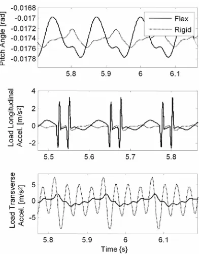
In order to excite the beaming mode closer to its 7.71

Hz natural frequency for the truck with 5000 kg payload, a new road is applied with 2 cm-high bumps spaced at 2.5 m (8 Hz excitation). A numerical linearization of the system, using 20 sim’s frequency domain toolbox, re- vealed a damping ratio of 23% for the beaming mode. For base excitation of a simple mass-spring-damper sys- tem with 23% damping, the maximum dynamic amplifi- cation factor would be approximately 2. Given the small magnitude of the beam vibration relative to rigid ele- ments, even a near-resonant excitation of the flexible modes would not cause unstable, large-amplitude motion; however, significant discrepancies may arise if a rigid model is used instead of a flexible model. Figure 16

shows the three vehicle responses from Figure 15 for

which there is significant disagreement between flexible and rigid models. The rigid model underpredicts peak-to- peak pitch angle variation (which is very small in either case). Longitudinal load acceleration peaks are predicted properly by the rigid model, but some transients between bumps are not captured. The rigid model shows an even more severe overprediction of transverse payload acce- leration than for the previous road.

An advantage of the bond graph approach in this paper is the ease with which individual flexible modes can be retained or eliminated. Figure 17 shows predictions of

the three responses from Figure 16 generated using all

Figure 16. Model responses, 2.5 m bump spacing.

Figure 17. Responses of 3-mode and 1-mode flexible model.

(modes 2 and 3 eliminated). Correct peak-to-peak mag- nitudes and frequency content can be given with a model of intermediate complexity compared to the rigid and three-mode flexible models.

The goal of the final simulation scenario is to investi- gate the effect of a road profile that excites the system near the resonance of a higher mode. Typically modes

from the first up to a certain number (e.g. modes 1-3) are retained, with higher ones eliminated. For some systems, depending on damping, an input with frequency content near the natural frequency of a mode may necessitate the retention of that mode, but allow the elimination of both lower and higher modes. Figure 18 plots results from 1

cm-high bumps spaced at 1 m, which for a 30 m/s vehi- cle speed corresponds to a 30 Hz input. Referring to Ta-ble 2, this should increase the participation of the second

flexible mode.

With the smaller, more closely spaced bumps, the rigid model predicts responses well with the exception of the payload transverse acceleration. The modal amplitudes ηi

show that for the 2.5 m bump spacing at 20 m/s (8 Hz), the second modal amplitude was 12% of the first modal amplitude. For the 1 m bump spacing at 30 m/s (30 Hz), the second modal amplitude was 44% of the first.

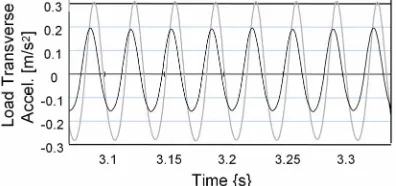
The approximate damping ratio of mode 2 is 77%, ex- plaining why, while more significant in a relative sense, the contribution of mode 2 did not exceed that of mode 1 despite excitation of mode 2 at resonance. For the 1 m bump spacing, eliminating mode 2 has a greater effect than before as shown in Figure 19. Flexible mode 2 is

essential for prediction of the payload acceleration.

6. Summary and Conclusions

A complete pitch plane vehicle model has been presented. The model contains longitudinal dynamics, pitch and bounce dynamics, and frame flexibility. Frame flexibility, normally included only in pitch plane models with no longitudinal degrees of freedom, is incorporated into the longitudinal portion of the model by treating beam transverse deflection as occurring perpendicular to an undeformed frame that can undergo large rigid body mo- tions. A modal expansion, based on an Euler-Bernoulli beam, models flexible motion as the sum of responses from decoupled oscillators each with modal stiffness, mass and damping. The bond graph formalism, while not required for implementation of the model, greatly facili- tates addition or subtraction of model elements (includ- ing modes) and reformulation of the equations. Superpo- sition of block diagrams atop the bond graph model, which is a feature of several commercial software pack- ages, allows simultaneous modification of model and controllers.

Figure 18. Bump spacing 1 m, velocity 30 m/s.

Figure 19. Transverse payload acceleration, 1 m bump spacing, 30 m/s velocity, flexible mode 2 eliminated (dark line) vs. all modes retained (light line).

would require a flexible model, as would prediction of higher-frequency vibrations that might affect noise, vi- bration and harshness or occupant comfort. The pre- sented model allows easy assessment of the effect of in- creasing or reducing complexity.

The greatest challenge in parameterizing the model would be the determination of modal parameters. While analytically tractable for a simple free-free beam, the calculation of natural frequencies and mode shapes of a complex truck frame is not straightforward. Cab and suspension attachment points, as well as the truck body, will have a stiffening effect. The payload mass, distribu- tion, and method of attachment to the truck will affect the quantities in question. If resources allow, the best ap- proaches would be frequency and mode shape extraction from a finite element model, or modal impact testing of an actual laden truck frame.

Future investigation will centre on the tire-road inter- action model, so that more complex road profiles not easily modeled as a sequence of slope values can be used. Tire models with more sophisticated treatment of the

enveloping of small bumps would improve prediction. An easy to use, predictive low-order model of such com- plex tire phenomena is in fact a goal of the larger vehicle dynamics community. Inclusion of future tire models in the current vehicle model would be straightforward using the bond graph approach, as would inclusion of more complex models of the engine, braking system, and sus- pension.

7. Acknowledgements

The author acknowledges the support of the Natural Sci- ence and Engineering Research Council of Canada under its Discovery Grant program, and the Auto21 Network of Centres of Excellence under project E301-EHV.

REFERENCES

[1] R. V. Field, et al., “Structural Dynamics Modeling and Testing of the Department of Energy Tractor/Trailer Combination,” Sandia National Laboratories Report SAND—96-2576C, CONF-970233, International Modal Analysis Conference, Orlando, 1997.

[2] R. V. Field, et al., “Analytical and Experimental Assess- ment of Heavy Truck Ride,” Sandia National Laborato- ries Report SAND—97-2667C, CONF-980224, Interna- tional Modal Analysis Conference, Santa Barbara, 1998. [3] M. Ahmadian and P. Patricio, “Dynamic Influence of

Frame Stiffness on Heavy Truck Ride Evaluation,” SAE Paper 2004-01-2623, Society of Automotive Engineers, Warrendale, 2004. doi:10.4271/2004-01-2623

[5] A. Dhir, “Nonlinear Ride Analysis of Heavy Vehicle Using Local Equivalent Linearization Technique,” Inter- national Journal of Vehicle Design, Vol. 13, No. 5, 1992, pp. 580-606.

[6] D. Margolis and D. Edeal, “Towards an Understanding of ‘Beaming’ in Large Trucks,” SAE Paper 902285, Society of Automotive Engineers, Warrendale, 1990.

[7] A. Costa Neto, et al., “A Study of Vibrational Behavior of a Medium Sized Truck Considering Frame Flexibility with the Use of ADAMS,” Proceedings of 1998 Interna- tional ADAMS User Conference, Ann Arbor, 1998. [8] A. Goodarzi and A. Jalali, “An Investigation of Body

Flexibility Effects on the Ride Comfort of Long Vehi- cles,” Proceedings of CSME Canadian Congress of Ap- plied Mechanics, CANCAM 2006, 2006.

[9] I. M. Ibrahim, et al., “Effect of Frame Flexibility on the Ride Vibration of Heavy Trucks,” Computers and Struc- tures, Vol. 58, No. 4, 1996, pp. 709-713.

doi:10.1016/0045-7949(95)00198-P

[10] I. M. Ibrahim, “A Generally Applicable 3D Truck Ride Simulation with Coupled Rigid Bodies and Finite Ele- ment Models,” International Journal of Heavy Vehicle Systems, Vol. 11, No. 1, 2004, pp. 67-85.

doi:10.1504/IJHVS.2004.004032

[11] D. G. Rideout, J. L. Stein and L. S. Louca, “System Parti- tioning and Improved Bond Graph Model Reduction Us- ing Junction Structure Power Flow,” Proceedings of ICBGM’05, International Conference on Bond Graph Modeling, New Orleans, 2005, pp. 43-50.

[12] D. G. Rideout and J. L. Stein, “Breaking Subgraph Loops for Bond Graph Model Partitioning,” Proceedings of ICBGM’07, International Conference on Bond Graph Modeling, San Diego, 2007, pp. 241-249.

[13] D. G. Rideout, J. L. Stein and L. S. Louca, “Extension and Application of an Algorithm for Systematic Identifi- cation of Weak Coupling and Partitions in Dynamic Sys- tem Models,” Simulation Modelling Practice and Theory, Vol. 17, 2009, pp. 271-292.

doi:10.1016/j.simpat.2007.10.004

[14] P. Michelberger, et al. “Dynamic Modelling of Commer- cial Road Vehicle Structures from Test Data,” SAE Pa- per 845120, Society of Automotive Engineers,

Warren-dale, 1984. doi:10.4271/845120

[15] T. Y. Yi, “Vehicle Dynamic Simulations Based on Flexi-ble and Rigid Multibody Models,” SAE Paper 2000- 01-0114, Society of Automotive Engineers, Warrendale, 2000.

[16] C. Cao, “Approaches to Reduce Truck Beaming,” SAE Paper 2005-01-0829. Society of Automotive Engineers, Warrendale, 2005. doi:10.4271/2005-01-0829

[17] J. Aurell, “The Influence of Warp Compliance on the Handling and Stability of Heavy Commercial Vehicles,” Proceedings of AVEC 2002, Hiroshima, 2002.

[18] D. Karnopp, et al. “System Dynamics—Modeling and Simulation of Mechatronic Systems,” 4th Edition, John Wiley and Sons, New York, 2006.

[19] 20 sim v.4.1.3.8, Controllab Products b.v., Enschede, 2011.

[20] L. S. Louca, et al., “Generating Proper Dynamic Models for Truck Mobility and Handling,” International Journal of Heavy Vehicle Systems, Vol. 11, No. 3-4, 2004, pp. 209-236. doi:10.1504/IJHVS.2004.005449

[21] D. Karnopp and D. Margolis, “Analysis and Simulation of Planar Mechanism Systems Using Bond Graphs,” Journal of Dynamic Systems, Measurement, and Control, Vol.101, No. 2, 1979, pp. 187-191.

[22] S. S. Rao, “Mechanical Vibrations,” 4th Edition, Pear- son-Prentice Hall, Upper Saddle River, 2004.

[23] H. Lee, “New Dynamic Modeling of Flexible-Link Ro- bots,” Journal of Dynamic Systems, Measurement, and Control, Vol. 127, No. 2, 2005, pp. 307-309.

doi:10.1115/1.1902843

[24] A. Yigit, et al. “Flexural Motion of a Radially Rotating Beam Attached to a Rigid Body,” Journal of Sound and Vibration, Vol. 121, No. 2, 1988, pp. 201-210.

doi:10.1016/S0022-460X(88)80024-5