TECHNICAL UNIVERSITY OF CLUJ-NAPOCA
ACTA TECHNICA NAPOCENSIS
Series: Applied Mathematics, Mechanics, and Engineering Vol. 60, Issue III, September, 2017
KINEMATICAL MODELLING FOR R2T SERIAL STRUCTURE
USED IN TRANSFER PARTS BETWEEN TWO WORKSTATIONS
Claudiu SCHONSTEIN, Nicolae PANC
Abstract: Based on the idea of bringing more flexibility to a working process, the paper is dedicated to the presentation of geometry and kinematics equations for a R2T serial structure, which can be used for carrying out tasks related to handling of pieces between two workstations. Thus, will be established in analytical form, the direct equations for geometric and kinematic model using dedicated algorithms, as the Transfer Matrices Algorithm and Iterative Algorithm. The Iterative Algorithm uses the outputs of the geometric study for realize the kinematic control, namely the establishment of linear and angular speed/acceleration of every kinetic joint of R2T robot and hence the TCP of the end effector.
Key words: serial structure, mathematical modeling, Transfer Matrices Algorithm, Iterative Algorithm.
1.INTRODUCTION
The industrial applications which are using robotic systems have developed continuously since the introduction of the first robotic device until today, because the use of industrial robots has beneficial effects in terms of increasing productivity and improving product quality.
Nowadays, when the robots have a higher and larger field of application day by day, the necessity for more and more precise and versatile robots is at peak. For this, the study of the robot precision is a required and a compulsory operation before even the prototype production of the structure taken into study. The large scale robot manufacturers invest big amounts of money in the perfecting of this field, the desired output being more and more precise robots.
Implementation of industrial robots in human areas activity has led to the development
of robotics research, hence in the most industrialized countries, the research in the field of robotics and consequently the flexible manufacturing systems, have developed a degree of diversification extremely high.
2. THE R2T TYPE SERIAL STRUCTURE
Further, in the paper is presented a solution of serial robot, which is intended to be used in transferring of parts between two sites.
The proposed robot, denoted R2T, is a cylindrical structure, is presented in Figure 1.
Figure 1 The R2T Serial Robot
0 O 0 x
0 z
According to the Figure 1, the mechanical structure can perform a rotation around O z0 0
axis and two translations; one along O z0 0axis, the other along O y0 0axis. As general features, the robot proposed for implementation in handling operations, has a total mass of 140 (kg) and overall dimensions
× × =0,5[ ] 0,3[ ] 1,15[ ]× ×
L l h m m m , with a payload
capacity of approximately 20 [kg].
3. MATHEMATICAL MODELLING OF
THE R2T SERIAL STRUCTURE
Further, using consecrated algorithms there are determined the direct and inverse geometry and kinematics equations, for the R2T mechanical structure proposed for implementation in an industrial handling process. The specific transfer matrix equation for a mechanical structure having rotational
( )
R or translational( )
T motions, according to [1]-[2], can be expressed using algorithms. These algorithms allowing detailed analysis, under numerical and/or graphical form, on geometry, kinematics and dynamics analyzed structure of any type and complexity.The obtained results, are essential to optimal design, dimensional aspect and energy, but also to simulate kinematic and dynamic behavior of mechanical structures.
3.1 Geometrical Modeling
The Direct Geometry Equations (DGM equations) can be determined by applying the Matrix of Locating Algorithm, taking into account the minimum number of, geometric or mechanical restrictions. Compared to other algorithms for geometric modeling, the Algorithm of Locating Matrix has a great advantage, especially in terms of mathematical calculus (is simplified). [2]
The situation matrix are defined as:
( ) ( )
1 0 0
1 1 0 0
1 ; 0
0 0 0 1 0 0 0 1
−
− −
−
= =
i
i i i i i i
i i i
R p R p
T T . (1)
Similarly, for i n= +1, the locating matrices between the frames
{ } {
n → n+1}
and{ } { }
0→ +n 1 are defined according to the following:( ) ( ) ( ) ( )
( ) ( ) ( ) ( )
0 0 0 0 1 1
0 0 0 0 10 0 1
0 0 0 1
0 0 0 1
n n n n n
n n n n
n s a p
T
n s a p
T T T
+ +
+ +
=
= ⋅ =
(2).
In the expressions (2), p( )0 is a vector which defines the position of the last joint with reference system attached to base of the robot, and npn( )0+1n characterizes the relative position of the system attached to end effector besides the geometrical center of the last joint.
For i = 1→n, the situating matrices between two close related system
{
i−1}
→{ }
i are defined as:(
;)
(
;)
(
1)
0 0 0 1
∆
⋅∆ −∆ ⋅ ⋅
=
i
i i i i i i
i i
R k q q k
T k q ; (3)
[ ]
(
)
1
1 ;
−
− ∆
= ⋅
i
i T Ti i T ki qi . (4)
According to [1]-[4], the rotation matrix between two neighboring reference frames is:
[ ]
{
(
) (
) (
)
}
1
; ; ; ; ;
−
= ⋅∆ ⋅∆ ⋅∆
i
i i i i i i i i i
i R R x q R y q R z q (5)
( )0
(
)
1 1
1 1
− −
−
= + − ∆ ⋅ ⋅
i i i
i i i i i i
r p q k . (6)
For i = 1→n, the position vector between
{ }
i and {i−1}with respect to{ }
0 fixed frame, respectively the position of joint{ }
i related to the same fixed frame is determined as:[ ] 0 1 1
1 1
− −
− = ⋅ −
i i
i i i i
p R r ; 1
1
− =
=
∑
i
i j j
j
p p .(7)
The situation matrix, between { }0 →{ }i is:
[ ] [ ] [ ]
0
0 1
1 0 0 0 1
−
=
= =
∏
i j i ii j
j
R p
and for the end-effector:
[ ] [ ] 0 0
1 1
0 0 0 1
+ +
= ⋅ =
n n n n
n s a p
T T T . (9)
The orienting vector is defined [1]-[4] with the following identity:
(
αA−βB−γC)
={
n+10[ ]
}
;ψ=(
α β γA B C)
TR R (10)
The DGM equations are included in the following generalized matrix:
0
ψ
α β γ
= =
T
x y z
T
x y z
p p p p
X . (11)
The Direct Geometrical Modeling (DGM), regardless of the algorithm used, aims to establish the geometry equations that will serve in determining the Direct Kinematic Model (DKM).
Geometrical Modeling of the robot had to be performed manually because of the multiple methods existent which allow the solving of this particular issue and also because of the inexistence of a generalized, computerized process able to perform it in the symbolical form [2]. The Geometrical Modeling for R2T mechanical structure is not a simple problem. This mathematical problem is solved in this work using the algebraic method. In the kinematic study of the work there can be used expressions obtained from the geometrical method due to their not so complicated expression and due to the simplicity of the algorithm that generated them.
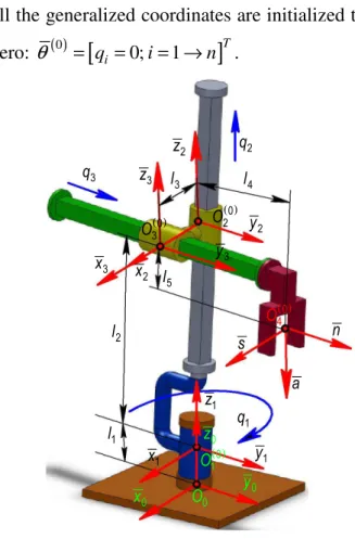
Further, will be established the DGM equations, for the R2T serial structure. According to the first step, related to any algorithm devoted MGD equations, it is represented in Figure 2, the kinematic scheme of the robot in the initial configuration, when
all the generalized coordinates are initialized to zero:
θ
( )0 =[
qi =0;i= →1 n]
T.According to the input data corresponding to DGM, the matrix of nominal geometry Mvn( )0 for R2T robot type proposed is given in Table 1.
Table 1. The matrix of nominal geometry
In keeping with Table 1, and Figure 2, the are highlighted the geometrical particularities for the R2T serial robot, as following:
1
l
0
O
( )0 4
O
2
q
1
q
a
s n
0
z
0
x y0
2
l
( )0 1
O
Figure 2 The kinematic scheme of R2T Robot proposed for handling parts
3
q
1
z
1
x y1
3
l l4
5
l
( )0 2
O ( )0
3
O
2
z
2
x
2
y
3
z
3
(
)
(
)
(
)
1 1 1
2 2 2
3 3 3
1; ; 1 ;
2; ; 0 ;
3; ; 0
= ≡ ∆ =
= ≡ ∆ =
= ≡ ∆ =
i k z
i k z
i k y
(12)
According to (1) there is established:
[ ]
10
1 1
1 1
1
c s 0 0
s c 0 0
0 0 1
0 0 0 1
q q
q q
l T
−
=
(13)
For the second joint, on the basis of (3), (4) and (1), there is obtained:
[ ]
2 1
2
2
1 0 0 0
0 1 0 0
0 0 1
0 0 0 1
q T
l
=
+
(14)
To establish the homogenous transformation matrix, there is used expression (8), which leads to:
[ ]
1 1
1 1
1 0
2 2
2
c s 0 0
s c 0 0
0 0 1
0 0 0 1
−
+ +
=
q q
q q
l l q
T (15)
According to (4) there is obtained:
[ ]
3
2
3
3
0 1 0 0 0 1 0 0 0 1 0 0 0 1
T
l q
=
; (16)
On the basis of the same expression (8) in keeping with (15) and (16), there is obtained:
[ ]
1 1 3 1 3 1
1 1 3 1 3 1
2 0
2 3
1
c s 0 c s
s c 0 c s
0 0 1
0 0 0 1
q q l q q q
q q q q l
T q
l l q
− −
+ +
⋅ ⋅
⋅ ⋅
=
+
(17)
For i=4, the situation matrices
{ }
4 →{ }
3 are:[ ]
3 4
43 4
5
0 1 0 0
1 0 0
0 0 1
0 0 0 1
l
T T
l
≡ =
− −
; (18)
which, in keeping with (17), according to (9), are leading to:
[ ]
[ ] [ ]
1 1 1 3 1 3 1 4 1
1 1 1 3 1 4 1 3 1
1 2 5 2
4
0 0 3
4 3 4
s c 0 c s c s
c s 0 s c
0
c s
0 0 1
0 0 0
0 1
1 0
q q q q q l q l q
q q q q q l q l q
l l l n s a p
T T
q T
− − + −
+ + +
−
= ⋅ = =
⋅ ⋅ ⋅
⋅ ⋅ ⋅
+ − +
=
(19)
In the expression, which characterize the location matrix (19), are included the rotation matrix 0
[ ]
4 R and the vector position p4. The
components of the two matrices are:
[ ]
10
1 4
1
1
s c 0
c s 0
0 0 1
−
−
=
R
q q
q q (20)
1 3 1 3 1 4 1
1 3 1 4 1 3 1
1 4
2 5 2
c s c s
s c c s
q q q l q l q
q q q l q l q
l l l q p
− + −
+ + +
+ −
⋅ ⋅ ⋅
= ⋅ ⋅ ⋅
+
(21)
representing the resulting orientation matrix (20) and the position vector (21), between
{ } { }
4 → 0 frames, both being included in the expression of the column vector of operational variables (11).According to [1], in order to establish the orientation angles, αx, βy, γz for exact determination of the values, there is used the trigonometric functionAtan 2, defined by:
(
)
[
]
{
}
[
]
{
}
[
]
{
}
[
]
{
}
; 0; 0 ;
/ 2 ; 0; 0 tan2 ;
; 0; 0 ;
/ 2 ; 0; 0
s c
s c
x A s c
s c
s c
α α α
π α α α
α α
π α α α
π α α α
≥ >
+ > <
= =
+ < <
− + < ≥
(22)
Hence, in keeping with (22), results:
(
)
(
)
tan 2 ; tan 2 0; 1
αx =A sαx cαx =A − =π
1
2
π
γz = +q , βy =0
( )
1 3 1 3 1 4 1
1 3 1 4 1 3 1
1 2 5 2
0
1
c s c s
s c c s
0
2
q q q l q l q
q q q l q
q l l l q X
q l
π
π
⋅ ⋅ ⋅
⋅ ⋅ ⋅
=
+
− + −
+ + +
+ − +
(23)
The expression (23) characterizes the Direct Geometric Modeling of the robot type RTT studied. Parameters included in (23) are expressing the position and orientation of the end effector minutiae to fixed reference system attached to the robot base.
The parameters included in (23) are expressing the position and orientation of the end effector with respect to the fixed reference system, attached to the base of the robot.
The study didn`t take into account the mechanical characteristics, and not imposed kinematic or dynamic restrictions. From the mathematical point of view, in the general case, the problem is reduced to solving a system of six algebraic linear equations with six unknowns.
3.2 Kinematical Modeling
In this paragraph will be established the operational kinematic parameters that express the movement of the end effector in Cartesian space. To define these parameters it is used the Iterative Algorithm. With this algorithm will be defined the kinematic parameters with respect to the fixed reference frame, attached to the base. The kinematic analysis take into account on one hand the position and orientation of each link necessary to describe the location of the end effector in the robot workspace, and on the other hand the speed variation of links throughout the working process. [5], [6].
In applying the iterative algorithm [3], in a first step, for the first joint, i=1 it has to be assumes that absolute kinematic parameter values corresponding to the fixed base of the mechanical structure of the robot are:
{
0 0 0 0}
0 0, 0 0, 0 0, 0 0
ω = ω& = v = v& = .
For i= →1 n, there are determined the angular and linear velocities which are defining the absolute motion of each kinetic link using the expressions :
[ ] 0
0 0
1
ω = ω− + ∆ ⋅ ⋅& ⋅ i i
i i i R qi ki (24)
(
) (
)
0 0 0 0
1 ω 1 1 1
− − −
= + × + − ∆ ⋅& ⋅
i i i ii i i i
v v p q k ; (25)
Similarly, for each i= →1 n, kinetic link of the robot, the corresponding angular and linear accelerations projected on the fixed reference system are defined as follows:
[ ] [ ]
{
0 0}
0 0 0
1 1
ω& = ω&− + ∆ ⋅ ω− × ⋅& ⋅ + ⋅&& ⋅
i i
i i
i i i i qi R ki qi R ki (26)
(
)
(
){
}
0 0 0 0 0
1 1 1 1 1 1
0 0 0
1 2
i i i ii i i ii
i i i i i i
v v p p
q k q k
ω ω ω
ω
− − − − − −
= + × + × × +
+ − ∆ ⋅ × ⋅ + ⋅
& & &
& && ; (27)
In the second part of the iterative algorithm, are determined the kinematic parameters, which characterize the movement in each i= →1 n kinetic link relative to the { }i
mobile reference system, as:
[ ]
[ ]
0 0 1
1 1
ω ω −ω
− −
= T⋅ = i ⋅ + ∆ ⋅& ⋅
i i i
i i R i i R i i qi ki; (28)
[ ]
[ ]
{
}
(
)
0 0 1 1 1
1 1 1
1
1
T i
i i i i
i i i i i i ii
i
i i i
v R v R v p
q k
ω
− − −
− − −
−
= ⋅ = ⋅ +⋅ × +
+ − ∆ ⋅ ⋅& .(29)
The expressions of angular and linear accelerations projected on the mobile reference system { }i , that characterizing the relative movement of each i= →1 n link are defined by the following expressions:
[ ] [ ]
[ ]
{
}
0 0 1
1 1
1
1 1
i
i i
i i
i i i
i i i i
i
i i i i i i
R R
R q k q k
ω ω ω
ω
−
− −
−
− −
= ⋅ = ⋅ +
+∆ ⋅ ⋅ × ⋅ + ⋅
& & &
& && ; (30)
[ ]
[ ]
{
}
(
) (
)
0 1 1 1
1 1 1
1 1
1 1 1
1 1 1
1 2
ω
ω ω
ω
− − −
− − −
− −
− − −
− − −
= ⋅ = ⋅ + × +
+ × × +
+ − ∆ ⋅ ⋅ × ⋅ + ⋅
&
& & &
& &&
i i
i i i i
i i i i i i ii
i i i
i i ii
i i i
i i i i i i
v R v R v p
p q k q k
In the last step of the iterative algorithm, the absolute motion of the final effector i=n is defined, taking into account the situation equations, respectively the absolute linear and angular velocities and accelerations (operating velocities and accelerations).
( )n0 ( )n0 T ( )n0 T T
n n
X& = v ω ; (32)
( )n0 ( )n0 T ( )n0 T T
n n
X&&= v& ω& . (33) Hence, in keeping with , (12), according to (24)-(27), for i=1 there are determined:
[ ] 0
0 0 1
1
1 0 1 1 1
1
0 0
ω = ω + ∆ ⋅ ⋅ ⋅ =
&
&
R q k q
; (34)
(
)
(
)
0 0 0 0
1 0 0 10 1 1 1 1
0 0 0 ω = + × + − ∆ ⋅ ⋅ = &
v v p q k (35)
[ ]
{
[ ]
}
(
)
0
0 0 0 1
1
1 0 1 0 1 1
0 1
1
1 1 0 0 1
T
q
q R k
q R k
ω = ω + ∆ ⋅ ω × ⋅ ⋅ +
+ ⋅ ⋅ =
& & &
&& &&
; (36)
(
)
(
)
{
[ ] [ ]}
(
)
0 0 0 0 0
1 0 0 10 0 0 10
0 0
0 1 1
1 1
1 1 1 1 1 1
1 2
0 0 0 T
v v p p
q R k q R k
ω ω ω
ω = + × + × × + + − ∆ ⋅ × ⋅ ⋅ + ⋅ ⋅ = = & & &
& && .(37)
On the basis of the same (24)-(27) and (12) for i=2, there is obtained:
[ ]
(
)
0 0 0
2 1 2 2 2
0
0 2
2
2 2 2 2 0 0 1
T
q k
R q k q
ω ω
ω
= + ∆ ⋅ ⋅ =
= + ∆ ⋅ ⋅ ⋅ =
&
& & ; (38)
(
)
(
)
0 0 0 0
2 1 1 21 2 2
2 2 1 0 0 ω = + × + −∆ ⋅ ⋅ = & & q
v v p q k (39)
[ ]
{
[ ]
}
(
)
0
0 0 0 2
2
2 1 2 1 2 2
0 2
2
2 2 0 0 1
T
q
q R k
q R k
ω = ω + ∆ ⋅ ω × ⋅ ⋅ +
+ ⋅ ⋅ =
& & &
&& &&
; (40)
(
)
(
)
{
[ ] [ ]}
(
)
0 0 0 0 0
2 1 1 21 1 1 21
0 0
0 2 2
2 2
2 2 2 2
2
2 2
1 2
0 0 q T
v v p p
q R k q R k
ω ω ω
ω = + × + × × + + −∆ ⋅ × ⋅ ⋅ + ⋅ ⋅ = = & & & & && && (41)
The third link is characterized by:
[ ]
(
)
0 0 0
3 3 3 3 3
0
0 3
3
3 3 3 3 0 0 1
T
q k
R q k q
ω ω
ω
= + ∆ ⋅ ⋅ =
= + ∆ ⋅ ⋅ ⋅ =
&
& & ; (42)
(
)
(
)
1 3 3 1 1 3 1 1
1
0 0 0 0
3 3 3 32 3 3 3
3 3 1 1 3 1 1
2
s s c
c c s
1
q q l q q q q q q q l q q q q q
v v p
q q k ω = + × + − − − ⋅ ⋅ ⋅ + ⋅ − ⋅ − ∆ ⋅ ⋅ = ⋅ ⋅ ⋅ ⋅ ⋅ = &
& & &
& & &
&
; (43)
[ ]
{
[ ]
}
(
)
0
0 0 0 3
3
3 2 3 2 3 3
0 3
3
3 3 0 0 2
T
q
q R k
q R k
ω = ω + ∆ ⋅ ω × ⋅ ⋅
+ ⋅ ⋅
+
=
& & &
&& &&
; (44)
(
)
(
)
{
[ ] [ ]}
1 1
1
1
3 1 3 1 3 1
3 1 3 1 1 3
3 1 3 1 1 3 1
3 1 3 1 1
0 0 0 0 0
3 2 2 32 2 2 32
0 0
0 3
1
3
3 3
3 3 3 3 3 3
2
2
( s c ) 2 c
( c s ) s
( c s 2 s
( s c ) c
1 2
)
q q l q q
v v p p
q R k q
q q q q q l q q q q
q q l q q q q q
q q l
k
q
R
q q
ω ω ω
ω = + × + × × + + −∆ ⋅ ⋅ × ⋅ ⋅ + ⋅ ⋅ = ⋅ ⋅ − ⋅ ⋅ ⋅ − − ⋅ − ⋅ ⋅ ⋅ − + ⋅ − ⋅ − ⋅ − ⋅ − ⋅ ⋅ ⋅ = ⋅ − − ⋅ ⋅ + ⋅ & & & & &&
& & && & && & &&
& && & && 3 2 q q && && (45)
According to [1], the end-effector of the serial structure has the following kinematical parameters: 3 1 0 0 4 0 0 ω ω = =
q&
; (46)
(
)
0 0 0
4 3 3 43
1 3 3 1 1 3 1 1
1 3 3 1 1 3 1 1
2
s s c
c c s
q q l q q q q q
q q l q q q q q
v p q v ω − − − ⋅ ⋅ ⋅ + ⋅ − ⋅ ⋅ = + × = ⋅ ⋅ ⋅ = ⋅
& & &
& & &
&
; (47)
(
)
0 0
4 3 0 0 1
ω& = ω& = &&q T; (48)
(
)
1 1
1
1
3 1 3 1 3 1
3 1 3 1 1 3
3 1 3 1 1 3 1
3 1 3
0 0 0 0 0
4 3 3 43
1 1 1 3
2
3 3 43
2
2
( s c ) 2 c
( c s ) s
( c s 2 s
( s
)
c ) c
q q l q q q q q
q q l q q q q
q q l q q q q q
q q l q
v v p p
q q q
q
ω ω ω
− ⋅ − ⋅ ⋅ ⋅ − + ⋅ − ⋅ = + × + × × = ⋅ ⋅ − ⋅ ⋅ ⋅ − = ⋅ ⋅ − ⋅ − ⋅ − ⋅ ⋅ ⋅ − − ⋅ + ⋅ & & &
& & && & && & &&
& && & && &&
&&
(49)
Thus, based on the RTT structure configuration, for i= →1 4 the following kinematic parameters characterizing the movement in driving joint, relative to the mobile reference system { }i , are determined as:
[ ]
(
)
0
1 0
1 1 1 0 0 1
[ ]
(
)
0
1 0
1= 1 ⋅ 1= 0 0 0
T T
v R v . (51)
[ ]
(
1)
0
1 0
1
1 1 0 0
ω& = R ⋅ ω& = &&q T; (52)
[ ]
(
)
1
1 0
1=0 ⋅ 1= 0 0 0
& & T
v R v (53)
[ ]
(
)
0
2 0
2 2 2 0 0 1
ω = R T⋅ ω = q& T; (54)
[ ]
(
)
0
2 0
2= 2 ⋅ 2= 0 0 &2
T T
v R v q . (55)
[ ]
(
1)
0
2 0
2
2 2 0 0
ω& = R ⋅ ω& = q&& T; (56)
[ ]
(
)
2
2 0
2 =0 ⋅ 2 = 0 0 2
& & && T
R v q
v (57)
[ ]
(
)
0
3 0
3 3 3 0 0 1
ω = R T⋅ ω = q& T; (58)
[ ]
3 1
3 0
3 0
3 1 3
2 3 3 T q q q v q q
v R l
⋅ = ⋅ = ⋅ − + & & & &
. (59)
[ ]
(
1)
0
3 0
3
3 3 0 0
ω& = R ⋅ ω& = q&& T; (60)
[ ]
2
3 1 3 1 3 1
2
3 1 3 1
0
3 0 3 3
3 3
2
2
l q q q q q
l q q q q
v R v
q ⋅ ⋅ ⋅ = ⋅ = ⋅ ⋅ − − ⋅ − − +
& && & && & & && & &&
&&
(61)
[ ]
(
)
0
4 0
4 4 4 0 0 1
ω = R T⋅ ω = q& T ; (62)
[ ]
3 1 3 1 1 4 1 1
1 3 1 4
0
4 0
4 4 4 1
2
c s
( s c )
T
l q q q q l q q
q q q
v v q
q R l ⋅ + + ⋅ + ⋅ − − + ⋅ ⋅ = ⋅ = ⋅
& & & &
& &
. (63)
[ ]
(
1)
0
4 0
4
4 4 0 0
ω& = ⋅ ω& = && T
q
R ; (64)
[ ]
2 2
1 1 1 1 3 1 3 1
2
3 4 1 1 4 1 1
2 2
1 1 3 1 1 1 1 3
2
3 1 4 1 1 4 1 1
2 4
4 0
4 0 4
s c
c s
s c 2
s c
q q q q l q q q q l q q l q q q q l q q q q q
q q l q q R q q v l v q + ⋅ + − + − ⋅ + ⋅ ⋅ ⋅ − − ⋅ − ⋅ − − ⋅ − ⋅ + ⋅ ⋅ ⋅ ⋅ ⋅ − = ⋅ = ⋅ ⋅ ⋅ ⋅
& && && & && & &&
&& & & & && & &
&& & && &&
(65)
The expressions (34)-(49), are defining the absolute motion of the end effector, taking into account the situating equations and absolute linear and angular accelerations and accelerations respectively.
Taking into account the relations (32) and (33), there are obtained:
1 3 3 1 1 3 1 1
1 3 3 1 1 3 1
0 1 0 2 4 0 4 1
s s c
c c s
0
0
q q l q q q q q q q l q q q q q
q q v X ω ⋅ ⋅ ⋅ ⋅ − − = = − ⋅ ⋅ ⋅ + ⋅ − ⋅ ⋅
& & &
& & &
& & & ;(66) 1 1 1 1
3 1 3 1 3 1
3 1 3 1 1 3
3 1 3 1 1 3 1
3 1 3 1 1 1 3
2 1 2 2 0 4 0 0 4
( s c ) 2 c
( c s ) s
( c s 2 s
( s ) 0 ) c 0 c
q q l q q q q q
q q l q q q q
q q l q q q q q
q q l q q q q
q q v X ω − ⋅ − ⋅ ⋅ ⋅ − + ⋅ − ⋅ − ⋅ − ⋅ − ⋅ ⋅ ⋅ − − ⋅ + ⋅ ⋅ ⋅ − ⋅ ⋅ ⋅ − ⋅ ⋅ = =
& & && & && & &&
& && & & && && && & && && (67)
The expressions previously determined are the Direct Kinematics Equations (DKM) that characterizing the absolute motion of the final effector and which will be used as input data in the dynamic modeling. The expressions (50)-(65), are defining the motion of the joint with respect to own reference frame. Taking into account equations (32) and (33), there can be expressed the operational speeds and accelerations, compared to the own system as:
3 1 3 1 1 4 1 1
1 3 1
4 4 4 4 4 4 1 2 1 c s
( s c )
0
0
l q q q q l q q
q q q l q
q v X q ω ⋅ ⋅ ⋅ = = + + ⋅ + ⋅ − − + ⋅
& & & &
& & & & (68) 2 2
1 1 1 1 3 1 3 1
2
3 4 1 1 4 1 1
2 2
1 1 3 1 1 1 1 3
2
3 1 4
4 1 1 4 1 1
2 4 4 1 4 4 s c c s
s c 2
s c
0
0
q q q q l q q q q l q q l q q q q l q q q q q
q q l q q l q q q q v X ω + ⋅ + − + − ⋅ + ⋅ − − ⋅ − ⋅ − − ⋅ ⋅ ⋅ ⋅ + ⋅ ⋅ ⋅ ⋅ ⋅ − ⋅ ⋅ ⋅ = = − ⋅
& && && & && & &&
4. CONCLUSION
The construction of capable robots in performing diverse tasks, with higher speed and precision is a global goal, thus being priority directions of research in robotics, in this context, it is obvious the complexity of the issues concerning the construction, the operation, and the control of robots.
In the paper, has been considered a serial structure of R2T type, which should be implemented in a handling process of parts between two workplaces. Direct Geometric Modeling, regardless of the algorithm used, aims to determine the direct geometry equations that will serve to determine the direct kinematic model. The geometric study did not take into account mechanical characteristics, and did not impose kinematic or dynamic restrictions. From a mathematical point of view, in the general case, the problem is reduced to solving an algebraic, nonlinear six-equation system with six unknowns.
For the proposed mechanical structure, have been determined the operational kinematic parameters, by expressing the final effector movement in Cartesian space, by using the
Iterative Algorithm. Hence, with this method, the kinematic parameters were defined both with respect to the fixed system { }0 and in relation to its own system{ }i , for each driving joint
( )
i .5. REFERENCES
[1] Negrean, I., Mecanică Avansată în Robotică, Ed. UT PRESS, ISBN 978-973-662-420-9. Cluj-Napoca, 2008. [2] NEGREAN, I., NEGREAN, D. C., The
Locating Matrix Algorithm in Robot Kinematics, Cluj-Napoca, October 2001, Acta Technica Napocensis, Series: Applied Mathematics and Mechanics, 2001
[3] Negrean, I, Vuşcan, I, Haiduc, N, Robotică. Modelarea cinematică şi dinamică, Editura Didactică şi Pedagogică, R.A., Bucureşi, 1997.
[4] Negrean, I., Schonstein, C., s.a., Mechanics
― Theory and Applications, Editura UT Press, 2015, 433 pag. ISBN 978-606-737-061-4.
[5] Megahed, S., Principles of Robot Modelling and Simulation, John Willy & Sons, 1993
[6] Schilling, J.R., Fundamentals of Robotics Analysis and Control, Pretince Hall Inc., 1990
Modelare cinematică pentru structura serială R2T utilizată pentru transferul pieselor
între două posturi de lucru
Rezumat: Plecând de la ideea de a aduce mai multă flexibilitate unui proces de lucru, lucrarea este dedicată
prezentării ecuaţiilor de geometrie şi cinematică pentru o structură serială R2T, care poate fi utilizată pentru îndeplinirea sarcinilor legate de manipularea pieselor între două posturi de lucru. Astfel, se vor stabili în formă analitică, ecuaţiile directe pentru modelul geometric şi cinematic folosind algoritmi dedicaţi, cum ar fi Algoritmul Matricelor de Transfer şi Algoritmul Iterativ. Algoritmul Iterativ utilizează rezultatele studiului geometric pentru a realiza controlul cinematic, adică stabilirea vitezei/acceleraţiilor liniare şi unghiulare a fiecărei articulaţii cinematice a robotului R2T şi prin urmare, a punctului caracteristic al efectorului final.
Claudiu SCHONSTEIN, Lecturer, Ph.D, Eng, Technical University of Cluj-Napoca, Department of Mechanical Systems Engineering, E-mail: [email protected], 103-105 No., Muncii Blvd., Office C103A, 400641, Cluj-Napoca.