TECHNICAL UNIVERSITY OF CLUJ-NAPOCA
ACTA TECHNICA NAPOCENSIS
Series: Applied Mathematics, Mechanics, and Engineering Vol. 62, Issue III, September, 2019
USING THE LINEAR PROGRAMMING TO DETERMINE THE
PRODUCTION PLAN OF THE ENTERPRISE
Călin Ciprian OȚEL
Abstract: Maximizing the profit is the desirability of any enterprise but this is not an easy task when it is desired to achieve several types of products and given that in the equation enters a series of variables such as: the available resources, the resource consumption for the product unit, the profit on each type of product that can be achieved, etc. Therefore the matter of identifying the optimal variant of the quantity of each type of product to be made so the profits earned by the enterprise to be maximum is searched. This paper deals with this problem by transposing data in the form of a mathematical programming problems. Key words: mathematical programming, linear programming, production plan.
1. INTRODUCTION
The production process can be defined as “the totality of the conscious actions of employees of an enterprise, realized with the help of different machines, equipment or installations upon the raw materials, materials or other components for the purpose of their transformation into products, works or services with a certain market value”.[11]
For the production process to be carried out in optimal conditions and in order to obtain a good productivity an enterprise needs a solid production plan, this because all the activities of the enterprise start from the production plan. Usually, a plan refers to materials, equipment, human resources, training, capacity and the ways to complete the work in a specific time.
That is why in order to achieve a continuous flow of work the production plan must take into account some key elements before the
production starts, such as: equipment
acquisition, material ordering, bottlenecks, procurement and training of the labor force.[10] Considering that when the production plan is realized, it is necessary to take into account a series of restrictions regarding the factors of production both in number and as a yield, a plan that has to aim the maximization of profits, it is
necessary to use optimization techniques (linear programming, PERT method, queuing theory, inventory optimization, etc.) and computer techniques (computer programs for optimal programming of production).
Linear programming is successfully used to optimize allocation of resources, to allocate production on different machines under conditions of maximizing profits, to determine the quantities of various goods to be produced, to transport products between working places and from there to the distribution points.[11]
By linear programming, it is intended to achieve aims under conditions of restrictions.
2. THE GENERAL FORM OF THE
MATHEMATICAL PROGRAMMING
PROBLEM
A problem of mathematical programming (optimization problem with restrictions) can be stated as follows:
Find the values of the variables x1,x2,..., xn that verify the restrictions given in the form of equality or inequality such as:
= ≥ ≤
0 ) x ( h
) 0 ( 0 ) x ( g
k i
p ,..., 2 , 1 K
m ,..., 2 , 1 i
= =
where x=(x1,x2,...,xn)∈M⊆Rn and which must achieve the maximum (minimum) of the objective function (scope) represented by function f.
The optimization problem with restrictions can be represented symbolically in the following way:
= ≥ ≤ →
0 ) x ( h
) 0 ( 0 ) x ( g
min(max) )
x ( f
k i
p ,..., 2 , 1 K
m ,..., 2 , 1 i
=
= (2)
n
R M x∈ ⊆
In some situations, variables may also be restricted by other conditions, such as those of non-negatives that may be applied to a part of the x vector components or to all components.
Mathematical programming problems can be classified into:
• Linear programming problems – when all the functions involved in (2) are linear functions of degree I;
• Nonlinear programming problems – when at
least one of the functions is nonlinear;
• Integer number programming problems –
when all variables x1, x2, ..., xn are required to
be integer numbers;
• Mixed programming problems – when only
some of the variables are integers;
• Real numbers programming problems –
when there are no special restrictions on variables;
• Deterministic programming problems – when
all functions from (2) have constant coefficients in their expression;
• Parametric programming problems – when
at least in one of these functions, the coefficients of the variables depend on a parameter;
• Stochastic programming problems – when at
least one of these functions has random variables with a known probabilistic distribution as coefficients.[1]
3. THE GENERAL FORM OF THE LINEAR PROGRAMMING PROBLEM
Linear programming models occupy a particularly important place, both in theory and in practice. These have allowed a thorough
analysis of the maximum efficiency of complex systems, the discovery of new concepts of the economic optimum and the improvement of research and knowledge methods.[9]
The linear programming problem is a problem in which the objective function is linear and the restrictions are linear functions of degree I, meaning:
=
⋅ =
= n
1 k
k
k x
c cx ) x (
f (3)
where:
) c ,..., c , c (
c = 1 2 n , x = (x1,x2,..., xn), and
=
− ⋅ = n
1 k
i k ik
i(x) a x b
g , i=1,2,...,m.
The problem can be stated: determine the maximum of function f on the set of restrictions
0 ) x (
gi ≤ , i=1,2,...,m.
The linear programming problem can be written in the following forms:[1]
• Canonical:
≥ ≤ ⋅
=
0 x , b x a cx
max(min) i
n
1 k
k
ik (4)
• Standard:
≥ = ⋅
=
0 x , b x a cx
max(min) i
n
1 k
k
ik (5)
As examples of linear programming
problems can be stated[9], [12]: the problem of the optimal production plan, the diet problem (of mixture), the problem of the optimal use of resources and the transport problem.
4. SOLVING LINEAR PROGRAMMING
PROBLEMS USING THE DUALITY
THEOREMS
The duality wants that for a primal problem (P) – which is a maximization problem with restrictions having the form: max{f(x): x
∈
Ω
}, to build a dual problem (D) – which is a minimization problem with restrictions having the form: min{f*(u): u∈
Ω
*} and the conditionsfor the two problems to comply with the following properties:
• for each x
∈
Ω
and for each u∈
Ω
* to be f(x)≤f*(u);
solution, and the optimal values of the objective functions are equal;
• if the dual problem has an optimal solution, then the primal problem has also an optimal solution, and the optimal values of the objective functions are equal.
The primal problem (P):
Max{cx: Ax≤b, x≥0} (can also be written as: min{-cx: -Ax≥-b, x≥0}), which has the dual (D) of form:
min{bTu: ATu≥cT, u≥0} (can also be written
as: max {-bTu: -ATu≤-c, u≥0}
For the two problems we have the following notations:
- c = (c1,c2,...,cn),
- x=(x1,x2,...,xn)T,
- A =(aik) a matrix of type (m×n),
- b=(b1,b2,...,bn)T
- f(x)=cx, an objective function for (P); - f*(u)= bTu, an objective function for (D);
-
Ω
={x∈ Rn: Ax≤b, x≥0}, the set of admissible solutions for (P);-
Ω
*={u∈Rm: ATu≥cT, u≥0}, the set ofadmissible solutions for (D);
- yi = - ai1x1 - ai2x2 - ... - ainxn + bi≥0, i = 1,2,...,m,
restrictions in (P);
- vi = a1ju1 + a2ju2 + ... + amjum – cj≥0, j = 1,2,...,n,
restrictions in (D);
The solving of a linear program of the form (P) is done with the simplex algorithm, which determines whether the program solution is optimal, and otherwise it shows the optimal infinite situation or actually builds a better solution than the current one, the simplex method being a systematic research process of linear program solutions.
A special quality of the simplex algorithm is that it produces not only the optimal solution to the problem to which it applies but also the optimal solution to the dual problem.
Simplex tables are used to manually solve small-scale linear programs, while for large-scale linear programs, computer programs are used to eliminate the "rough" calculations inherent in solving this algorithm.
Further, the simplex table attached to the two problems is provided:
Table 1. Simplex table
v1 = v2 = ... vs = ... vn = f* =
-x1 -x2 ... -xs ... -xn 1
u1, y1 = a11 a12 ... a1s ... a1n b1
u2, y2 = a21 a22 ... a2s ... a2n b2
... ... ... ... ... ... ... ... ...
ur, yr = ar1 ar2 ... ars ... arn br
... ... ... ... ... ... ... ... ...
um, ym = am1 am2 ... ams ... amn bm
1, f = -c1 -c2 ... -cs ... -cn 0
In order to build the dual of a linear programming problem, the following should be taken into account:[1]
a) the variables number of the dual is equal to the constraints number of the primal problem;
b) the constraints number of the dual is equal to the variables number of the primal problem;
c) the matrix of the dual is the transpose of the primal matrix;
d) to each equality of the form i
n
1 j
j ij x b
a ⋅ ≤
=
with i∈{1,2,...,m1} from the primal
problem corresponds in the dual the variable ui ≥ 0, i = 1,2,...,m;
e) to each equality of the form i
n
1 j
j ij x b
a ⋅ ≤
=
with i∈{m1+1,...,m} from the primal
corresponds the variable ui, i = m1+1,...,m,
f) to each primal variable xj≥0, j∈{1,2,...,n}
corresponds in the dual an equation of
form j
m
1 i
i ij u c
a ⋅ =
=
.
To solve a primal problem (P) of the form max{cx: Ax≤b, x≥0} three stages must be passed through:
I. Elimination of independent variables
n 2 1,x ,..., x
x , is no longer necessary because
these variables are subject to non-negativity restrictions, meaning xj≥0.
II. Determination of an admissible solution. At this stage, the choice of the pivot element is sought, so that after a finite number of steps a basic solution is obtained or is found out that the system is incompatible.
Be the dual of a linear programming problem written in the form of:
Table 2. The dual of a linear programming problem
u1 u2 … us … un 1
v1 = a11 a12 ... a1s ... a1n d1
v2 = a21 a22 ... a2s ... a2n d2
... ... ... ... ... ... ... ... vr = ar1 ar2 ... ars ... arn dr
... ... ... ... ... ... ... ... vm = am1 am2 ... ams ... amn dm
f* = q
1 q2 ... qs ... qn 0
The pivot elements are chosen according to the minimal ratio rule, which is built between the last line and the pivot line:
≠ > =
≤
≤ a 0,a 0
q min a
q
is is
i
m i 1 rs
r , (6)
where: s = Gauss-Jordan number of steps; so in order to find the basic admissible solution, the last line from Table 2 is analyzed.
If the line of objective function (f*) is
positive, this step is not necessary, and even under these conditions the rule of the minimum ratio will continue to be used.
III. Improvement of the admissible solution
and finding the optimal solution.
This stage will start when at the end of the second stage, the following situation will be encountered in the resulting table: d1
≥
0, d2≥
0,… , dm
≥
0. To find the optimal solution, the lastcolumn will be analyzed. If all the values on this
column are positive, then the problem has the optimal solution. To determine this, proceed as follows: the elements ui from above the table
will be zero, and for the elements ui that are to
the left of the table the values are read from the table, from the column "1".
After choosing the pivot element, marked by framing the pivot element into a square, a Gauss-Jordan step is performed according to the rules:
1) the pivot element is replaced by 1;
2) the other elements in the pivot column
remain unchanged;
3) the other elements in the pivot line change the sign;
4) the elements of the other lines and columns are calculated with the formula:
rs rk
is ik ik
a a
a a
b = (7)
The main diagonal must be considered to be always the diagonal with the pivot element (ars).
5) all the elements of the new table are divided with the pivot element.
5. CASE STUDY
Knowing that an enterprise produces 4 types of products P1, P2, P3, P4, for which 5 resources
R1, R2, R3, R4 and R5 are used, it is desired to
determine a production plan so the benefit obtained by the enterprise to be maximum. The data of the available quantities of the 5 resources, resource consumption for the product unit and the benefit to be achieved by selling a quantity of each product type are given in the following table:
Table 3. Data of the problem
Products
Resources P1 P2 P3 P4 Available
R1 1 2 4 3 12
R2 3 5 1 0 30
R3 0 1 2 4 9
R4 1 2 1 3 10
R5 1 1 4 1 8
Benefit 2 3 4 1
and the objective function is:
2x1+3x2+4x3+x4→max, function which aims to
The objective function is written together with the constraints system and so the primal problem (P) is obtained:
max x
4x 3x
2x1+ 2+ 3+ 4→ (8)
≥ ≥ ≥ ≥ ≤ + + + ≤ + + + ≤ + + ≤ + + ≤ + + + 0 x , 0 x , 0 x , 0 x 8 x 4x x x 10 x 3 x x 2 x 9 x 4 2x x 30 x x 5 3x 12 x 3 4x x 2 x 4 3 2 1 4 3 2 1 4 3 2 1 4 3 2 3 2 1 4 3 2 1 (9)
In the above system, x1, …, x4 are the
quantities that need to be produced from the products P1, …, P4 in conformity with the 5
restrictions that occur due to the available resources for each product. In addition, it must be taken into account that these quantities can only have positive values, which is why to the system will be added the conditions of
non-negativity
x
1≥
0
,
x
2≥
0
,
x
3≥
0
,
x
4≥
0
.The dual problem (D) is associated to the primal problem: min u 8 u 10 u 9 u 30
12u1 + 2 + 3 + 4 + 5 → (10)
≥ ≥ ≥ ≥ ≥ ≥ − + + + + ≥ − + + + + ≥ − + + + + ≥ − + + + + 0 u , 0 u , 0 u , 0 u , 0 u 0 1 u 3u 4u 3u 0 4 u 4 u 2u u 4u 0 3 u 2u u u 5 2u 0 2 u u u 3 u 5 4 3 2 1 5 4 3 1 5 4 3 2 1 5 4 3 2 1 5 4 2 1 (11) Table 4. Simplex table attached to the dual u1 u2 u3 u4 u5 1
v1 = 1 3 0 1 1 -2
v2 = 2 5 1 2 1 -3
v3 = 4 1 2 1 4 -4
v4 = 3 0 4 3 1 -1
f* = 12 30 9 10 8 0
Because the objective function line is positive, stage II is not required. It can be seen that the elements from column "1" are negative,
which is why it can move to stage III.
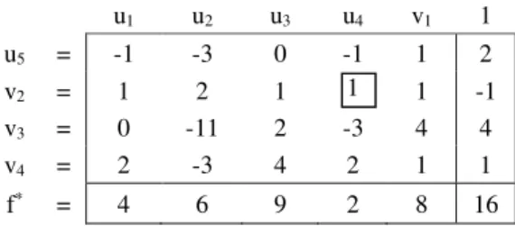
It is chosen as the pivot line, the first line of Table 4, and then reports with the objective function line are built. According to these reports, it follows that the element 1 from column u5 should be chosen as the pivot element. Table 5. Simplex table after making a Gauss-Jordan step
u1 u2 u3 u4 v1 1
u5 = -1 -3 0 -1 1 2
v2 = 1 2 1 1 1 -1
v3 = 0 -11 2 -3 4 4
v4 = 2 -3 4 2 1 1
f* = 4 6 9 2 8 16
In Table 5 it is found that in the second line, in column "1" the element is negative, therefore the second line is chosen as the pivot line, and the element 1 from the column u4 as the pivot
element.
Table 6. Simplex table after making one more Gauss-Jordan step
u1 u2 u3 v2 v1 1
u5 = 0 -1 1 -1 2 1
u4 = -1 -2 -1 1 -1 1
v3 = 3 -5 5 -3 7 7
v4 = 0 -7 2 2 -1 3
f* = 2 2 7 2 6 18
The optimal solution to the dual problem is: u1=0, u2=0, u3=0, u4=1, u5=1.min f*= 18 = f*(0, 0, 0, 1, 1)
The optimal solution to the primal problem is:x1=6, x2=2, x3=0, x4=0.
max f = 18 = f(6, 2, 0, 0)
6. CONCLUSIONS
The maximum benefit obtained by the enterprise is 18 monetary units, and in order to achieve this benefit 8 products: 6 of P1, 2 of P2
and 0 of P3 and P4 have to be realized.
minimize the total amount of the consumed resources. Therefore, analyzing Table 3 from the statement of the problem, it can be found the following:
• for product P1, 6 units of resources are
consumed with a benefit of 2 units;
• for product P2, 11 units of resources are
consumed with a benefit of 3 units;
• for product P3, 12 units of resources are
consumed with a benefit of 4 units;
• for product P4, 11 units of resources are
consumed with a benefit of 1 unit. In the final result are found:
• product P1 with a minimum resource
consumption of 6;
• product P2 which has the same resource
consumption of 11, as well as the product P4, but has a superior benefit.
7. REFERENCES
[1] Blaga, L., Lupșa, L., Elemente de programare
liniară, Editura Risoprint, ISBN 973-656-328-6, Cluj-Napoca, 2003.
[2] Bogdan, Ș., Morar, L., Bogdan, M.,
Organizational change, a mathematical model for the optimal resources sharing, Acta Technica Napocensis, Series-Applied Mathematics, Mechanics and Engineering, ISSN: 1221-5872 Volume: 58, Issue: 3, pp. 369-374, 2015. [3] Filip, D., Applying to the mathematical methods
to optimize the launching process in manufacturing, Acta Technica Napocensis, Series-Applied Mathematics, Mechanics and
Engineering,ISSN: 1221-5872 Volume: 61, Issue: 4, pp. 585-592, 2018.
[4] Hernández-Lerma, O., Lasserre J.B., The Linear
Programming Approach. In: Feinberg E.A., Shwartz A. (eds) Handbook of Markov Decision Processes. International Series in Operations Research & Management Science, vol 40. Springer, Boston, MA, pp. 377-407, 2002. [5] Lungu, F., Abrudan, I.,(coord.),...Oțel, C.C.,
Ingineria sistemelor de producție – Îndrumător de
laborator, Editura Todesco, ISBN 987-606-595-025-2, Cluj-Napoca, 2013.
[6] Oţel, C.C., Management industrial – îndrumător
pentru studenți / Industrial management – guide
for students, Editura Digital Data Cluj, ISBN 978-973-7768-96-4, Cluj-Napoca, 2018.
[7] Rusan, R., Blebea, I., Estimating the importance
of the attributes of a new product in development process, Acta Technica Napocensis, Series-Applied Mathematics, Mechanics and Engineering, ISSN: 1221-5872 Volume: 59, Issue: 2, pp. 223-228, 2016.
[8] Wu, JA., Linear Programming Solving the
Optimization Question of Production Plan,
International Conference on Materials Science and Engineering Science, Book Series: Advanced Materials Research, Part: 1, 2, Volume: 179-180, pp. 1162-1166, ISBN 978-3-03785-016-9, Shenzhen, R China, 2010.
[9] www.asecib.ase.ro/Mitrut%20Dorin/Curs/ bazeCO/doc/23PL.doc
[10] https://www.bdc.ca/en/articles-tools/opera tions/operational-efficiency/pages/production -plan-top-tips-improving-operations.aspx [11] http://cis01.central.ucv.ro/csv/curs/ei/c8.html [12] http://cis01.central.ucv.ro/csv/curs/mat_ts/
mat_ts.doc
Utilizarea programării liniare pentru determinarea planului de producție al întreprinderii
Rezumat: Maximizarea profitului este dezideratul oricărei întreprinderi dar acest lucru nu este o sarcină ușoară atunci când se dorește realizarea mai multor tipuri de produse și având în vedere că în ecuație intră o serie de variabile precum: resursele disponibile, consumurile de resurse pe unitatea de produs, profitul pe fiecare tip de produs ce se poate obține, etc. De aceea, se pune problema identificării variantei optime a cantității din fiecare tip de produs care trebuie realizată astfel încât profitul obținut de companie să fie maxim. Lucrarea de față tratează această problemă prin transpunerea datelor sub forma unei probleme de programare matematică.