Talley_Trey.pdf

(1)

Anticipating Mixed Use Water Demand:

Chapel Hill & Carrboro, NC

By

Trey Talley

A paper submitted to the faculty of

The University of North Carolina at Chapel Hill in partial fulfillment of the requirements for the degree

Master of City and Regional Planning

April 7, 2017

This paper represents work done by a UNC-Chapel Hill Master of City and Regional Planning student. It is not a formal report of the Department of City and Regional Planning, nor is it the

(2)

Anticipating Mixed Use Water Demand:

Chapel Hill & Carrboro, NC

Department of City & Regional Planning

UNC Chapel Hill

Trey Talley

Land Use & Environmental Planning

(3)

Acronyms

ASHRAE American Society of Heating, Refrigerating, and Air-Conditioning Engineers AWE Alliance for Water Efficiency

AWWA American Water Works Association BAU Business as Usual

BGD Billion Gallons per Day C&I Commercial and Institutional DU Dwelling Unit

EPA U.S. Environmental Protection Agency EPAct U.S. Energy Policy Act of 1992

FFL Florida-Friendly Landscaping Program FTE Full-Time Equivalent

GBIG Green Building Information Gateway GPCD Gallons per Capital per Day

GPF Gallons per Flush

GPHSF Gallons per Heated Square Foot GPM Gallons per Minute

GPU Gallons per Unit

HMXD High-Density Mixed Use HSF Heated Square Foot/Feet

KGPHSF Thousand Gallons per Heated Square Foot KGPSF Thousand Gallons per Square Foot

KGPU Thousand Gallons per Unit

LEED Leadership in Energy and Environmental Design MFR Multifamily

MGD Million Gallons per Day MXD Mixed Use

MXDR Mixed-Use Residential

OWASA Orange Water and Sewer Authority RES Residential

SF Square Foot/Feet

SFR Single Family Residential TOD Transit Oriented Development TRWSP Triangle Regional Water Supply Plan UHI Urban Heat Island

(5)

1 | P a g e

Introduction

This report provides an overview of factors affecting water demand in mixed use developments in order to support the Orange Water and Sewer Authority’s (OWASA) ongoing efforts to update their existing Long Range Water Supply Plan. The update will extend demand projections out to 2065, and will inform future decisions regarding water resources and the potential provision of additional incentives for improved water efficiency in the OWASA service area. Given the recent trend of increased mixed use development in Chapel Hill and Carrboro, OWASA officials are interested in both the historical demand patterns of existing developments as well as

information about current industry standards for estimating water demand from mixed use properties. The overarching goal is therefore to provide context for the development of more accurate water demand assumptions for modern mixed use properties.

(6)

2 | P a g e

Factors Affecting Mixed Use Water Demand

Trends in Water Use

According to the United States Geological Survey (USGS), approximately 57 percent—or 23.8 billion gallons per day (bgd)—of water withdrawn for public supply in the United States in 2010 was delivered for domestic use (USGS, 2014a). This figure includes both indoor and outdoor uses such as drinking water, sanitation, and landscaping for residential customers nationwide (USGS, 2014a). OWASA’s 50-year projections from 2011 show a total demand for raw water of 10.8-15.0 million gallons per day (mgd) in 2060, representing a substantial decrease from prior long-term estimates of 14.6-16.6 mgd in 2050 (OWASA Staff 2011, 3).

This reduction is largely attributed to an observed increase in water efficiency of 20-25 percent across all sectors (OWASA Staff 2011, 3), and fits with national trends in both total and per capita water use. A 2015 report by the Pacific Institute shows that total water use in the United States “peaked in 1980 at 440 bgd before falling to 400 bgd in 1985” (Donnelly and Cooley, 2015, 1). Total water use stayed somewhat flat between 1985 and 2005, before declining to 350 bgd in 2010 (Donnelly and Cooley, 2015, 1). National per capita water use also peaked in 1980 at 1,900 gallons per capita per day (gpcd), before falling to 1,100 gpcd by 2010 (Donnelly and Cooley, 2015, 1). Notably, nationwide per capita water use decreased by approximately 17 percent between 2005 and 2010, representing the largest decline in any five-year period (Donnelly and Cooley, 2015, 1).

Water use by the municipal and industrial sector—which includes residential use—accounted for only 19 percent of nationwide demand in 2010, but decreased by 4 percent from 2005 levels (Donnelly and Cooley 2015, 6). In fact, “per capita [municipal and industrial] water use has declined in every five-year period over the last three decades, from 360 gpcd in 1980 to 220 gpcd in 2010” (Donnelly and Cooley 2015, 6). Total national water use by the residential sector alone increased steadily between 1950 and 2005, while per capita demand remained somewhat steady at approximately 100 gpcd (Donnelly and Cooley 2015, 7). Between 2005 and 2010, however, “residential per capita water use declined by 7 percent, or 2 bgd, despite continued population growth, reducing per capita water use to 88 gpcd in 2010” (Donnelly and Cooley 2015, 8). These national figures, however, provide a somewhat skewed picture of trends in water use, as

significant efficiency gains in most parts of the United States were offset by population increases in relatively hot and dry parts of the country. According to the USGS, per capita domestic water use ranged from a high of 168 gpcd in Idaho to a low of 51 gpcd in Wisconsin (USGS, 2014b). The State of North Carolina fell on the lower end of 2010 per capita domestic water use rates at approximately 70 gpcd, or 18 gpcd below the national average (USGS, 2014b).

As planners and other public officials consider options for ensuring adequate drinking water supplies and resiliency against drought, it is important to understand not only the impacts of increased efficiency at the building level, but also the potential impacts of broad changes in land use mixes and shifting development trends. Improved understanding of these factors will

contribute to more accurate long term demand projections and help officials plan capital

investments for infrastructure related to raw water supplies, treatment facilities, and distribution networks. While it is important to research key drivers of water demand in all types of

(7)

3 | P a g e

urban development. Toward that end, the following subsections review literature from academic journals and publications by practitioners developing water supply plans for utilities and

governments across the United States. The review is organized according to scale, beginning with key factors affecting water use at the building level and expanding outward to site characteristics and local institutional context.

Building Level Factors

Water demand at the building level is influenced by multiple factors including fixtures and amenities, landscaping features, and unit types and management practices. One helpful way of considering building level determinants of water consumption is to draw a distinction between efficiency and conservation, where efficiency is largely defined on a physical input versus output basis, while conservation is viewed more as a set of behavioral patterns and choices (Alliance for Water Efficiency, 2016). This subsection provides an overview of recent research on the impacts of both physical and non-physical factors affecting water demand in mixed use properties.

Fixtures & Amenities

In mixed use properties, one relevant factor is the efficiency of fixtures and amenities that draw water for recreation, sanitation, drinking, cooking, cooling, and other common non-industrial uses. In a 2016 review titled The Status of Legislation, Regulation, Codes & Standards on Indoor Plumbing Water Efficiency, the Alliance for Water Efficiency (AWE) outlined the progression of efficiency requirements for water-consuming plumbing products and appliances from 1980 to 2015 (Table 1). Included directly from the AWE report, this table uses ‘gpf’ to indicate ‘gallons per flush’ and ‘gpm’ to indicate gallons per minute (Alliance for Water Efficiency, 2016, 2).

Table 1: Water Consumption by Water-Using Plumbing Products and Appliances: 1980 - 2015

Residential Bathroom

Lavatory

3.5+ gpm 2.5 gpm 2.2 gpm 2.2 gpm 1.5 gpm 57%

Showerhead 3.5+ gpm 3.5 gpm 2.5 gpm 2.5 gpm 2.0 gpm 43%

Toilet -

Residential 5.0+ gpm 3.5 gpf 1.6 gpf 1.6 gpf 1.28 gpf 74% Toilet -

Commercial 5.0+ gpm 3.5 gpf 1.6 gpf 1.6 gpf 1.6 gpf 68%

Urinal 1.5 to 3.0+ gpm

1.5 to

3.0 gpf 1.0 gpf 1.0 gpf 0.5 gpf 67%

Commercial Lavatory

Faucet

3.5+ gpm 2.5 gpm 2.2 gpm 0.5 gpm 0.5 gpm 86%

Food Service Pre-Rise Spray

Valve

5.0+ gpm No Requirement 1.6 gpm

(EPAct 2005) No Requirement 1.3 gpm 74%

Residential Clothes Washer

51

gallons/load No Requirement

26 gallons/load (2012 standard)

No Requirement 16

gallons/load 67%

Residential Dishwasher

14

gallons/cycle No Requirement

6.5 gallons/cycle

(2012 standard) No Requirement

(8)

4 | P a g e

The substantial reductions visible in Table 1 help explain why nationwide water use has declined since the 1980’s, as new construction must adhere to at least the minimum federal standards established by the U.S. Energy Policy Act of 1992 (EPAct). An AWE news release from 2014 analyzing national water savings 20 years after the implementation of the EPAct, argues that the 54 percent reduction from 3.5 gpf to 1.6 gpf toilets alone “saved the nation 18.2 trillion gallons of water…enough to supply the cities of Los Angeles, Chicago and New York for 20 years” (Alliance for Water Efficiency, 2014). A more comprehensive study performed by the American Water Works Association (AWWA) in 2001, estimated that the “national plumbing efficiency standards [would] reduce water production by about 8 percent by the year 2020, or 3.5 billion gallons per day” (Maddaus et al., 2001). Again, these savings vary by region such that areas with a higher percentage of indoor versus outdoor water use are expected to realize greater benefits from improved plumbing efficiency. The AWWA report reviews 16 case studies from utilities across the United States, including the nearby Town of Cary, NC, which had the highest

anticipated reduction rate of all 16 utilities at 9.1 percent in 2020 (Maddaus et al., 2001, 22). The report’s findings for the Town of Cary were higher than the 7.2 to 8.4 percent savings estimated in the AWWA’s analysis of the EPA region including North Carolina, potentially suggesting that the state may be among the largest beneficiaries of the EPAct efficiency standards (Maddaus et al., 2001, 25).

While some state and local governments have enacted rules that establish higher efficiency standards, the State of North Carolina only requires compliance with the minimum federal standards (Alliance for Water Efficiency, 2012). There are, however, multiple voluntary

programs with significant participation rates that encourage consumers and developers to pursue higher levels of water efficiency for fixtures, appliances, and even entire developments. For example, the U.S. Environmental Protection Agency (EPA) created the WaterSense Program in 2006. This program is designed to enable consumers to conserve water by certifying products and services that are at least 20 percent more efficient than federal standards without sacrificing performance (National Conference of State Legislatures, 2015). For toilets, this means that all dual or single flush toilets that use 1.28 gpf or less may possess the WaterSense label, because they use only 80 percent of the 1.6 gpf federal standard. The EPA estimates that the use of WaterSense fixtures and appliances saved approximately 1.5 trillion gallons of water nationwide from 2006 to 2015 (U.S. Environmental Protection Agency, 2015).

Multiple academic studies have confirmed the effectiveness of water conservation programs designed to increase the uptake of high efficiency fixtures and appliances among consumers. In recent research on the impacts of a retrofit and rebate program for high efficiency appliances by the Miami-Dade Water and Sewer Department, Lee et al. found that “the average water savings for the first year of installation [were] 4.24%, 5.45% and 5.17% for showerhead, toilet and washer programs, respectively” (Lee et al., 2011). Another article on the impact of a similar rebate program in Albuquerque, New Mexico by Price et al. compares the water savings from rebate programs in three separate categories: indoor, outdoor, and xeriscape (Price et al., 2014). The authors’ goal was to determine which categories of rebate programs were the most effective in yielding substantial water savings, as well as establishing whether or not these savings

(9)

5 | P a g e

After controlling for the price of water and local weather conditions, they found that low-flow toilets had “the greatest impact on water use, while low-flow washing machines, dishwashers, showerheads, and xeriscape [had] smaller but significant effects” (Price et al., 2014). Notably, they also found that “air conditioning systems, hot water recirculators, and rain barrels [had] no significant impact on water use” (Price et al., 2014).

Considered along with the other findings presented above, these studies suggest that the

efficiency of plumbing fixtures within a structure have a large impact on total water demand, and that even seemingly small efficiency upgrades can yield substantial water savings over time. In mixed use buildings, the initial installation of high-efficiency water-using fixtures may therefore lead to a substantially lower average annual demand rate. Officials seeking to estimate or

influence the amount of water use from an individual development should consequently examine the types and numbers of each fixture being installed. That said, there are other physical

characteristics of mixed use buildings that could impact average annual demand.

For example, the presence of certain amenities such as pools or cooling towers can increase water demand. The amount of water necessary to fill a swimming pool can be easily determined based on the total volume of the pool itself, and the most significant draws come when the pool is actually being filled. The more complicated factor related to swimming pools is the amount of water that is lost to evaporation, and therefore must be replaced on an ongoing basis. Prior studies have shown that evaporation depends upon multiple factors including pool location (i.e. indoor versus outdoor), pool occupancy, pool size, water and air temperature, and airflow from wind or ventilation systems (Shah, 2014). In a survey conducted by Fannie Mae in 2012, researchers found that the median annual water use per unit for multifamily properties that provided information on pools varied from 42.7 thousand gallons per unit (kgpu) for those with no pool, to 46 kgpu for properties with one pool, and up to 64.6 kgpu for properties with two or more pools (Fannie Mae, 2014).

Another potential source of water demand—especially in multistory mixed use buildings—is the use of water-cooled climate control systems. One popular form employs a combination of chillers, cooling towers, and air handling units to circulate chilled water throughout a building in order to reduce indoor air temperatures without the use of a more traditional air conditioning system. The primary driver behind the increased use of this type of climate control system is the fact that “evaporative water-cooled systems consume approximately half the overall energy of comparably sized air-cooled systems, yielding substantial lifecycle cost savings” (Furlong and Morrison, 2005). Closed-loop systems work by sending water through a condenser and

(10)

6 | P a g e Landscaping

The largest potential source of non-swimming-pool-related outdoor water use in mixed use buildings is irrigation and landscaping. Indeed, the EPA estimates that landscape irrigation represents approximately one-third of all residential water use nationwide, and that outdoor use by households in dry climates like the southwest may account for as much as 60 percent of all household water demand (U.S. Environmental Protection Agency, 2013a). In North Carolina, outdoor water use is estimated to account for an average of 20 to 30 percent of total water used in a given facility, and can peak to as much as 70 percent in the summer growing season (N.C. Division of Pollution Prevention and Environmental Assistance, 2009). For mixed use properties in OWASA’s service area, the most important factors to consider are the irrigation methods employed, the amount of vegetated area, and the type of vegetation that is present on the property. It is also worth noting that irrigation water demands may change over time, as not all landscaping and irrigation elements may be installed immediately after the end of construction.

Irrigation Methods

In a 1999 report sponsored by the AWWA Research Foundation titled Residential End Uses of Water, Mayer et al. reviewed the impacts of various irrigation methods on outdoor water use by single family residential consumers. While there are certainly some differences between

irrigation for single family properties and mixed use properties, the following general relationships included directly from the AWWA report should be rather consistent:

 Homes with in-ground sprinkler systems use 35 percent more water outdoors than those who do not have an in-ground system

 Households that employ an automatic timer to control their irrigation systems used 47 percent more water outdoors than those that do not

 Households with drip irrigation systems use 16 percent more water outdoors than those without drip irrigation systems

 Households who water with a hand-held hose use 33 percent less water outdoors than other households

 Households who maintain a garden use 30 percent more water outdoors than those without a garden

 Households with access to another, non-utility, water source displayed 25 percent lower outdoor use than those who used only utility-supplied water (Mayer et al, 1999)

(11)

7 | P a g e

More recent research on local outdoor water demand adds further nuance to past findings on the impacts of different irrigation methods. For example, a 2015 report in the Journal of Irrigation and Drainage Engineering analyzed the impacts of multiple ‘smart irrigation’ technologies on water consumption for 24 residential sites in Cary, North Carolina during the spring and summer months of 2009. For this study, Nautiyal et al., compared water savings from the following three irrigation system types against a control group: (1) standard irrigation controller with a soil moisture sensor; (2) standard irrigation controller with an evapotranspiration-based adjustment sensor; and, (3) standard irrigation controller using seasonal runtimes based on historical climate data. The control group consisted of systems with a standard irrigation control system with no additional sensors or interventions. The authors found that the soil moisture sensing system was the most efficient and used approximately 42 percent less water than the control group, while the other two system types saved water at a significant, yet lower rate (Nautiyal et al., 2015). These findings unsurprisingly suggest that new irrigation technologies are more efficient than those evaluated by Mayer et al. in 1999. Again, this study was conducted on residential properties, but its implications for irrigation demands by new mixed use developments may be substantial. Indeed, since the cost of installing more advanced irrigation systems could be spread across multiple tenants, uptake rates for soil moisture sensors among mixed use property owners could be higher.

Vegetated Areas

Mayer et al. also found that “the amount of water used for outdoor purposes (primarily irrigation) is positively related to the size of the lot…and the percentage of the lot that is irrigable

landscape” (Mayer et al., 1999). These relationships appear rather obvious since more water should be necessary to irrigate larger areas and no water would be intentionally used to irrigate non-vegetated surfaces. The more interesting factor at play is that different types of vegetation have been shown to require—or at least appear to require—more water to maintain aesthetic qualities. For example, a 2013 study published by the AWWA titled Residential Landscape Water Use in 13 North Carolina Communities, found that “residents whose lawns consisted of cool-season grass used more water on average during the growing season than residents whose lawns consisted of warm-season grass” (Fair and Safley, 2013). In the OWASA service area, surveyed residents with cool-season grass used an average of 6,100 gallons per month while those with warm-season grass only used an average of 5,400 gallons per month (Fair and Safley, 2013). The authors reasoned that “this could be because homeowners may observe cool-season species showing signs of stress more quickly during a drought than warm-season species and therefore apply larger quantities of water” (Fair and Safley, 2013). Given that OWASA

customers were shown to have smaller lawns than any of the other communities included in the study, and that certain mixed-use developments (see site context section below) might have larger vegetated areas than single-family homes, the choice of grass type could be an important factor in determining future demands.

(12)

8 | P a g e

from xeriscaping of around 55.8 gallons per square foot (Mayer et al., 2015). They noted, however, that much of the research on outdoor water savings from alternative urban landscaping uses inconsistent measurements and has been concentrated in only three states: Florida,

California, and Nevada (Mayer et al., 2015). That said, in a 2014 article referenced by the AWE, Boyer et al., found that residential participants in the Florida-Friendly Landscaping (FFL) program used 50 percent less water for irrigation on average, and that this figure increased to 76 percent compared to properties with ‘high-quality’ turf grass when only ‘good’ examples of FFL participants were considered (Boyer et al., 2014). Viewed in combination with other research on landscaping demands, it appears that there is a significant opportunity to reduce water demand from new mixed use developments by encouraging developers to install irrigation systems with soil moisture sensors, reduce total irrigable areas, and utilize a combination of warm-season turf grass and native vegetation.

Unit Types & Management

Another set of building level factors that affect water demand in mixed use properties includes the types of residential and non-residential units available, as well as management and design practices that may influence building efficiency or tenant behavior. One major factor in this category is a developer’s option to pursue non-compulsory efficiency and conservation programs such as certifications administered by various public and private organizations.

Residential Units

Residential portions of mixed use properties may take the form of condominiums or apartments, and vary in count, square footage, number of bedrooms, and total occupancy. While there is a substantial amount of research around residential water use, interpretation of this research for multifamily properties is rather difficult. One factor contributing to this difficulty is the fact that multifamily and single family water use are often lumped together into the same ‘residential’ category. Also, there appears to be no agreed-upon standard for per unit demand (i.e. per square foot, per dwelling unit, per capita, etc.), and data limitations may prevent researchers from identifying the amount of water drawn by individual users or for different uses. For example, in a 2012 survey of energy and water use in over 1,000 multifamily properties across the United States, Fannie Mae found that over 70 percent of respondents providing 12 months of meter data did not differentiate between indoor and outdoor use (Fannie Mae, 2014).

(13)

9 | P a g e

Tables 2 & 3: 2012 Fannie Mae Median Multifamily Annual Water Use Rates

As expected, there was substantial variation in annual usage rates between individual

properties/respondents. For annual per square foot water use, rates ranged from 0.017 thousand gallons per square foot (kgpsf) for the 5th percentile to 0.113 kgpsf for the 95th percentile. For annual per unit water use, rates ranged from 15.3 thousand gallons per unit (kgpu) for the 5th percentile to 98.2 kgpu for the 95th percentile (Fannie Mae, 2014, 7). As expected, there were notable variations in demand according to location and building type. Annual per square foot and per unit usage rates were highest in the West, and second highest in the South. The median annual rates for the South were 0.044 kgpsf and 44.5 kgpu (Fannie Mae, 2014, 22). Results for usage rates by building type were also interesting. On a per square foot basis, the survey found annual demands of 0.048, 0.047, and 0.039 kgpsf for low-rise, mid-rise, and high-rise properties, respectively. For per unit demand, the survey found annual rates of 45.6, 35.4, and 40.2 kgpu for low-rise, mid-rise, and high-rise properties, respectively (Fannie Mae, 2014, 23).

While these figures display substantial variation in usage rates, the story behind them makes sense given the information already presented above. Indeed, water usage is predictably higher in warmer climates, and low-rise multifamily properties are more likely to have vegetated areas that require water for irrigation. Along similar lines, it makes sense that the survey would find

evidence that annual usage rates are higher for properties with more bedrooms and residents per unit (Fannie Mae, 2014, 24). This relationship has been confirmed by other studies that have found that adding more residents to each unit creates diminishing increases in water use, and that children and retirement-age adults are among the highest water users (Klein et al, 2006, 27)

Non-Residential Units

Nonresidential portions of mixed use properties often include a combination of retail stores, restaurants, office spaces, and even hotels. In many cases, units designated for these purposes are located on the first few floors of the property, with residential units located above. Other mixed use developments may consist entirely of nonresidential units with retail stores and restaurants again on the first few floors and then office space or hotels on the remaining floors. The water use patterns of these nonresidential units can vary substantially not only from the water demands of the residential portions of mixed use properties, but also between nonresidential units of different types. As noted in a 2009 EPA report on water efficiency in the commercial and institutional (C&I) sector, one challenge in determining the water demands of these customer types is that “the definition of the sector varies among water utilities and in water use literature” (EPA WaterSense, 2009). Another challenge—illustrated in Table 4 adapted from the EPA report—is that there are substantial differences in the end uses of water for relevant C&I subsectors (EPA WaterSense, 2009). Note that there is some overlap in reported end use categories.

National 44.2 0.047

Northeast 34.7 0.037

Midwest 35.8 0.044

South 44.5 0.044

West 50.7 0.055

Region Gallons/Unit (000's)

(14)

10 | P a g e

Table 4: End Uses of Water in Relevant C&I Subsectors

In a 2010 study using a combination of statewide parcel-level land use characteristics and historic water consumption data from two major utilities, Morales and Heaney calculated

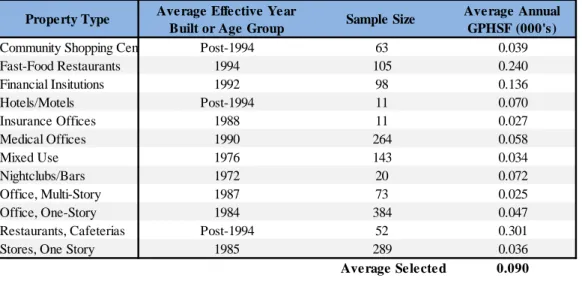
average water use rates for a wide range of C&I facilities across the State of Florida. These water use rates are included in Table 5 below (Morales and Heaney, 2010). The rates included in Table 5 have been converted to thousands of gallons per year in order to facilitate comparisons with other rates included in this report. It should also be noted that—unlike the Fannie Mae report on multifamily water use—the rates reported in this study are based on the ‘heated square feet’ of each property, rather than total square feet or number of units. There was, however, a strong relationship between heated area and total area, as heated square feet represented an average of 93 percent of total square feet across all C&I subsectors included in the analysis (Morales and Heaney, 2010).

Table 5: Average Water Use Rates for Selected C&I Subsectors in Florida

It is notable that the C&I subsectors which are most likely to be included in mixed use properties have a higher average annual use than the sector as a whole. Although there are likely

differences between water use patterns in Florida and North Carolina, these differences may be smaller for C&I users given that outdoor water use is lower for this sector than for residential users. Indeed, many C&I properties utilize outdoor areas more for parking than for landscaping. There may, however, be some variation between water use rates caused by higher evaporation rates from cooling towers in Florida, but as the authors note, cooling towers are generally only

End Use Office Buildings Restaurants Hotels

Cooling & Heating 28% 1% 11%

Domestic/Restroom 37% 31% 30%

Kitchen 13% 48% 14%

Landscaping 22% 4% 16%

Laundry N/A N/A 16%

Other N/A 8% 12%

Swimming Pools N/A N/A 1%

Washing & Sanitation N/A 4% N/A

Total 100% 96% 100%

Community Shopping Centers Post-1994 63 0.039 Fast-Food Restaurants 1994 105 0.240 Financial Insitutions 1992 98 0.136 Hotels/Motels Post-1994 11 0.070 Insurance Offices 1988 11 0.027 Medical Offices 1990 264 0.058 Mixed Use 1976 143 0.034 Nightclubs/Bars 1972 20 0.072 Office, Multi-Story 1987 73 0.025 Office, One-Story 1984 384 0.047 Restaurants, Cafeterias Post-1994 52 0.301 Stores, One Story 1985 289 0.036

Average Selected 0.090 Total All C&I 0.049 Property Type Average Effective Year

Built or Age Group

(15)

11 | P a g e

present in larger commercial establishments (Morales and Heaney, 2010). As expected, Morales and Heaney found that there were meaningful differences in the water use patterns of C&I properties based on the year in which they were built. The average age of the properties included in the Florida study are therefore included in Table 5, and when possible, only the average water use rate for the most recent age group is included.

Management & Design Practices

One important trend affecting water efficiency in both residential and commercial properties is the growing popularity of noncompulsory efficiency targets and certifications such as the LEED program administered by the US Green Building Council (USGBC). Developers and property managers have recognized such certifications as an effective means of signaling their

commitment to conservation to both tenants and public officials. According to the Green

Building Information Gateway (GBIG), 852 LEED certified activities covering nearly 92 million square feet have been recognized in North Carolina as of March, 2017 (GBIG, 2017a). Notably, 21 of these certified activities are located in Chapel Hill and Carrboro, representing over 1.5 million square feet of property in OWASA’s service area (GBIG, 2017b; GBIG, 2017c).

In general, LEED and other certification systems are designed as ‘point systems’ whereby certification is achieved through an accumulation of points awarded for installing specific features or achieving predetermined benchmarks. For water use, the USGBC awards credits related to indoor water use, outdoor water use, and metering technologies. The general

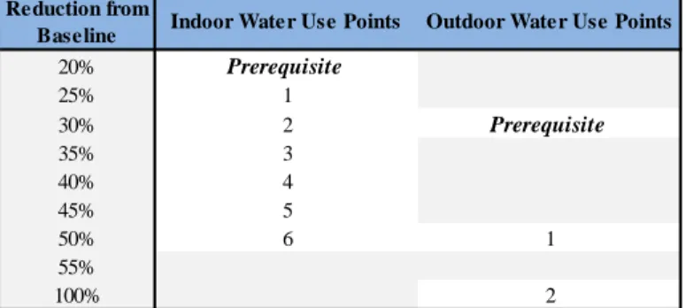
requirements for indoor and outdoor water efficiency credits in the LEED Building Design and Construction program are summarized in Table 6 (USGBC, 2017a). All reduction percentages in Table 6 are calculated from a baseline derived from the requirements of the EPAct. Metering requirements apply only to whole property water use, although a building may receive one point for metering two or more of the following subsystems: (1) Irrigation; (2) Indoor plumbing; (3) Domestic hot water; (4) Boilers; (5) Reclaimed water; and (6) Other process water (USGBC 2017b; USGBC 2017c). Additionally, a building may receive up to two points for limiting use by cooling towers (USGBC, 2017d). To place these points in perspective, the required number of points for each certification level are: Certified (40-49 points), Silver (50-59 points), Gold (60-79 points), and Platinum (80+ points) (USGBC, 2017e). It can therefore be said that while water efficiency is an important component of the LEED program, water efficiency upgrades account for a relatively small portion of the total points necessary for higher certification levels.

Table 6: Selected LEED BD+C Water Efficiency Requirements & Credits

Another noncompulsory management practice that affects water consumption rates is the way residents and tenants are metered and billed for water use. According to the National Conference

20% Prerequisite

25% 1

30% 2 Prerequisite

35% 3

40% 4

45% 5

50% 6 1

55%

100% 2

Reduction from

(16)

12 | P a g e

of State Legislators, the State of North Carolina requires individual meters for electricity and natural gas service for each dwelling unit, effectively banning the use of master meters for those services (National Conference of State Legislatures, 2016). There is, however, no such statewide requirement for water service. That said, the Town of Boone, North Carolina does have a local ordinance—passed in 2012—that requires individual metering for all new commercial and residential water customers, including those in mixed use developments (National Conference of State Legislatures, 2016; Boone, North Carolina, Code of Ordinances §50.109). Submetering programs are intended to more equitably distribute water expenses among residents and tenants by creating a more direct link between the amount of water used and the amount they are billed for that use. The resulting increase in information available to residents and tenants then enables them to make better decisions about their own consumption patterns. In a 2004 national study on submetering practices that controlled for other factors such as number of bedrooms, the year in which the property was built, and average water prices, researchers found that submetering reduced water use by between 5.55 to 17.5 kgpu each year, or 11 to 26 percent (Mayer et al., 2004, xxiii). The same study also found that submetering was somewhat uncommon, with only 3.9 percent of properties indicating that they submeter water compared to 84.8 percent that indicated including water costs in rent (Mayer et al., 2004, xxi).

Site Context

The preceding sections have primarily focused on the determinants of water use for individual structures without considering the location of those structures, or the potential interactive effects of increasingly dense urban development patterns. Some of these effects are straightforward. For example, since the “convenience of [having] live-work-play options in a single location,” and the potential to reduce traffic congestion are two of the most attractive features of mixed use

development, there is pressure to select sites in central urban locations rather than Greenfields (Rabianski and Clements, 2007). Such sites are less likely to have large vegetated areas, and can therefore be expected to exhibit lower rates of outdoor water use. What is less clear, however, is the way patterns of individual siting decisions may build up over time, and how resulting

alterations to the urban form could impact water use overall.

Density & Urban Heat Islands

Recent research on the impacts of ‘Smart Growth’ as an alternative to traditional urban sprawl sheds some light on the water-saving potential of higher-density urban environments. Before reviewing the findings of these studies, however, it is worth noting that most of the research in this area is model-based, and therefore should be viewed as informed conjecture rather than empirical truth. In a 2013 article comparing estimates of water use in suburban Boston under different scenarios of urban development, Runfola et al. found that “differences in lawn cover, living unit density, and the number of bathrooms [could] explain 90% of the variation in annual residential water use” (Runfola et al., 2013). Extrapolating out to 2030, the researchers estimated that the Town of Ipswich, MA could achieve a 5 percent reduction in water use through

(17)

13 | P a g e

and Chester, 2014). Overall, they estimated that switching from BAU to TOD development patterns would result in a decrease in total residential water consumption from 45,400 to 28,700 million gallons per year, a decrease of approximately 37 percent (Nahlik and Chester, 2014, 67). Obviously, there is a significant difference between the savings calculated in these two studies, but given known differences in usage rates by region, I would expect savings from densification in OWASA’s service area to be closer to the 5 percent in MA than the 37 percent in AZ.

There may, however, be some downsides to increased densification through the impacts of the ‘Urban Heat Island’ (UHI) effect. In general, UHI effects are relative increases in ambient temperatures caused by higher heat absorption rates and lower heat release rates in urban versus natural environments. This effect “can occur throughout the year, is affected by local weather conditions, and is typically most intense in the urban core and less severe on the urban

periphery” (Guhathakurta and Gober, 2007). Factors related to mixed use development that might increase UHI effects include construction materials, building heights and spacing, and increased impervious surfaces. In a 2007 study again focused on Phoenix, AZ, Guhathakurta and Gober found that:

A 1° F increase in a tract’s low temperature increases average water use in single-family units by 1.7% or 290 gallons for the typical single family unit for the month, holding all else constant. The difference between daily high and low temperatures, the second measure of UHI, resulted in greater changes in water use. If the difference between high and low temperature declines by 1° F, reflecting warmer nighttime temperatures, average water use in single-family units increases by 681 gallons. (Guhathakurta and Gober, 2007, 326).

It is important to note two aspects of these results. First, the reported water use increases are for single-family units, so mixed use developments with less vegetated area would likely exhibit less dramatic increases in water use. Second—and perhaps more importantly—UHI effects from increased urban development densities have the potential to increase water consumption rates in surrounding buildings, even those of a different development type. In Chapel Hill, there are already examples of mixed use developments that directly abut existing single family properties, so it would be interesting to see if water consumption in those properties has increased over time (see Greenbridge property profile).

One way of attenuating the UHI effect is to plant vegetation or install features that increase shade on vegetated and non-vegetated areas. A recent study conducted in Israel compared the cooling efficiency of different combinations of vegetation and shading techniques and calculated impacts on water use. The study concluded that while unshaded grass in courtyards had very little cooling effect and required the highest amount of water, combining grass courtyards with trees or mesh that shaded the grass substantially cooled the area and resulted in a more than 50 percent reduction in total water use (Shashua-Bar et al., 2009). Like most of the other studies in this section, this area-cooling research was conducted in a hot and dry environment, so I would expect the effects of both UHI and any mitigation strategies to be less pronounced in OWASA’s service area.

Institutional Context & Conservation

(18)

14 | P a g e

price of water, the presence of various conservation incentives, and residents’ awareness of water issues. Based on the information already presented, the impacts of pricing factors may be less pronounced in mixed use developments. I expect this to be the case because indoor uses are less discretionary than outdoor uses (Mayer et al, 1999), and households living in mixed use

developments are less likely to have yards than households living in single family homes. Also— as previously noted—the billing systems applied in multifamily housing do not always provide a clear price signal to individual users. Nonetheless, it is worth briefly reviewing those factors that appear most relevant to future development in OWASA’s service area.

Economic & Financial Factors

In a 2006 paper titled Factors Influencing Residential Water Demand: A Review of the

Literature, Klein et al. provide a helpful summary of existing research on the role of water prices and pricing structures in determining water demand. As with most other determinants of water demand, the authors note that household responsiveness to changes in water prices varies substantially according to multiple factors including season, geographic location, and

socioeconomic characteristics (Klein et al., 2006). Two patterns, however, have emerged that are consistent across most studies: (1) residential customers areresponsive to changes in price; and, (2) demand for water is relatively inelastic, meaning that the percentage change in demand is less than the percentage change in price (Klein et al., 2006, 6-7). The second point highlights the fact that there is some level of demand that is necessary rather than discretionary. Simply put,

regardless of the price of water, households must use at least a certain volume to cover basic needs such as sanitation, cooking, and drinking, while they may choose to skip watering their lawn if the cost is too high.

Seasonal differences in price elasticity are therefore often attributed to increased outdoor use in the spring and summer months (Klein et al., 2006). Klein et al. report that estimates of price elasticity are often “5-10 times higher during summer months as compared to those obtained for winter” (Klein et al., 2006, 7). Geographic differences in price elasticities are also often

attributed to the impacts of outdoor uses, albeit less confidently because of confounding

variables that aren’t always included in available data (Klein et al., 2006). That said, according to a 1992 study cited by Klein et al., residential water users in southern and western states “were more than twice as responsive to changes in price than residents throughout the rest of the United States” (Klein et al., 2006, 7). In a study in nearby Raleigh, NC, Danielson estimated the price elasticity of water to be approximately -0.27 for total water use, and -1.38 for outdoor sprinkling demand (Danielson, 1979). This means that—as expected—water demand at the household level was relatively inelastic, but irrigation-specific demands were elastic, and therefore more

susceptible to changes in price. Notably, Danielson’s estimate of -0.27 is close to 50 percent of the average -0.51 price elasticity calculated in a 1997 meta-analysis by Espey et al. (Espey et al., 1997, 1370), which conforms with expectations that the price elasticity of water is lower in the south.

(19)

15 | P a g e

block rate [are] 5 times more sensitive to changes in price than households facing a uniform rate structure” (Klein et al., 2006). It should be noted, however, that much of the research on

residential water price elasticity has been focused on single family homes or residential properties in aggregate, and therefore may have limited applicability for housing in mixed use developments. Research pertinent to the price elasticity of water used by the nonresidential portions of mixed use properties suggests that most commercial and office uses are relatively inelastic (Mitchell and Chesnutt, 2009). The following major points about commercial and industrial uses are helpfully included in a White Paper available through the AWE:

 Industrial demand tends to be less price inelastic than commercial demand, though demand for certain industrial processes requiring very high quality water can be very inelastic.

 Commercial demand tends to be inelastic, though empirical estimates span a wide range. Commercial water demand studies reviewed by Renzetti (2002) reported price elasticities ranging from 0.1 to 0.9. Elasticity varied considerably by commercial sector.

 As with residential customer demand for water, commercial and industrial demands are less inelastic in the long-run than in the short run (Mitchell and Chesnutt, 2009, 4).

Overall, while pricing factors and elasticities are important, they may not be as important as other factors affecting demand by mixed use buildings in OWASA’s service area. Indeed, given the area’s focus on retail and office spaces, most of the water use for both residential and

nonresidential units in new mixed use buildings is likely to be indoor and nondiscretionary.

Local Knowledge & Awareness

Utilities and other organizations have also sought to influence water use through non-price mechanisms such as public education campaigns, and voluntary or mandatory water use restrictions. Perhaps with the exception of mandatory restrictions, this type of conservation program is often seen as more politically feasible than increasing water prices, although there is some evidence to suggest that “using prices to manage water demand is more cost effective than implementing nonprice conservation programs” (Olmstead and Stavins, 2009). Again turning to the review provided by Klein et al., the authors found that studies of mandatory water use

restriction programs yielded savings of 13 to 64 percent, while studies of savings from voluntary programs and public information campaigns found a range of impacts from a net increase of 7 percent to 33 percent savings (Klein et al, 2006, 17). One potential explanation for the net increase in water use observed by some studies is that consumers may interpret information campaigns or voluntary restrictions as meaning that more stringent restrictions will be

implemented in the future, leading them to increase use in anticipation of decreased access in the future (Klein et al, 2006, 14).

Fair and Safley’s 2013 article provides some indication of how well price and non-price

(20)

16 | P a g e

Table 7: Fair and Safley Survey Responses by OWASA Customers

Here we see that 68 percent of customers were unaware of the restrictions that had been implemented, and 14 percent were unsure if there were any restrictions. Interestingly, more customers indicated that they had changed their indoor habits than their outdoor habits. This is strange given that outdoor use is generally considered more discretionary than indoor use, and that OWASA customers had the smallest lawns of all 13 North Carolina communities included in the study. Perhaps having smaller lawns led customers to believe that their impact on water supplies would be limited. Overall, the effects of price and non-price mechanisms for

encouraging water conservation can be described as mixed, and it is not immediately clear that their impacts on water use would be substantially different for mixed use developments than other property types.

Response Aware of Water Restrictions

Changed Outdoor Habits

Changed Indoor Habits

Yes 18% 39% 53%

No 68% 59% 47%

Did Not Know 14% 2% 0%

(21)

17 | P a g e

Anticipating Mixed Use Water Demand in OWASA’s Service Area

The previous section provided an overview of factors that affect water consumption rates according to features within individual structures, the locational context of those structures, and the institutional factors at play in a given locality. One primary takeaway is that water use is complicated, and actual consumption rates can vary substantially from one development to the next. Recognizing this fact, most utilities and public officials rely upon average usage rates to project future water demand instead of trying to calculate precise figures for water use by each existing or potential development in their service area. While a comprehensive review of all common demand estimation methodologies is beyond the scope of this report, it is worth briefly reviewing some common assumptions and methodologies employed by local utilities and selected organizations around the country.

Annual Demand Assumptions

This subsection includes a series of tables summarizing the demand projection assumptions used by several local water suppliers during preparation of the 2012 Triangle Regional Water Supply Plan (Triangle J Council of Governments, 2012). These tables only provide local estimates because—as previously noted—there are wide variations in water consumption rates by location, and national averages are skewed upward by the inclusion of relatively high-water-using areas in the Western part of the country. Since it is rare for organizations to have specific assumptions for mixed use properties, the rates included herein are for each of the individual uses that are

commonly included in mixed use developments: Residential, Commercial, and Institutional. Assumptions from OWASA are excluded from this section because they were based on ‘meter equivalents’ and officials have indicated that they wish to move away from this approach.

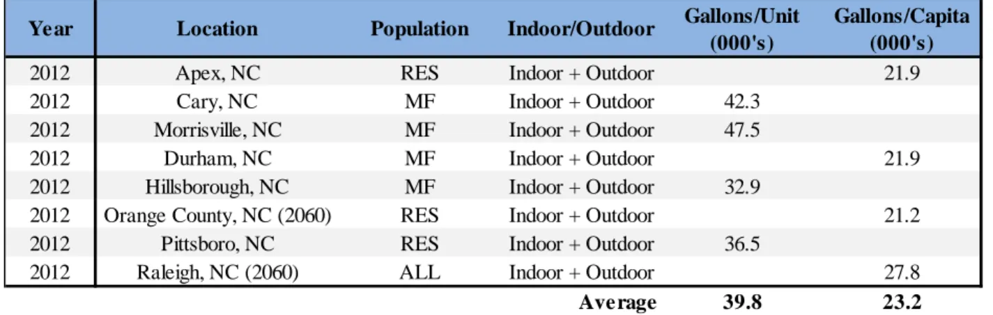
Table 8: Local Residential Annual Demand Assumptions

Table 8 above lists local annual demand assumptions for residential properties. It is interesting to note that organizations within the same region are using not only different types of rates for residential (i.e. both gallons per unit and gallons per capita), but also that these assumptions can vary by many thousands of gallons per year. One potential explanation for this variation is that each municipality likely has different mixes of multifamily or residential property types. For example, Morrisville may have a higher percentage of low-rise multifamily properties than Cary. Another potential source of the variation could be the general location of these properties within the urban environment. It stands to reason that if a municipality has a higher percentage of multifamily properties in the urban core than along the periphery, then the average amount of

2012 Apex, NC RES Indoor + Outdoor 21.9

2012 Cary, NC MF Indoor + Outdoor 42.3

2012 Morrisville, NC MF Indoor + Outdoor 47.5

2012 Durham, NC MF Indoor + Outdoor 21.9

2012 Hillsborough, NC MF Indoor + Outdoor 32.9

2012 Orange County, NC (2060) RES Indoor + Outdoor 21.2

2012 Pittsboro, NC RES Indoor + Outdoor 36.5

2012 Raleigh, NC (2060) ALL Indoor + Outdoor 27.8

Average 39.8 23.2

Year Location Population Indoor/Outdoor Gallons/Unit (000's)

(22)

18 | P a g e

vegetated land—and therefore average annual outdoor use—per property would be lower and vice versa. Additionally, there could be substantial differences in the average age of the properties in each municipality, which could lead to the presence of more or less efficient fixtures.

Table 9: Local Commercial Annual Demand Assumptions

As with the residential demand assumptions, there is substantial variation in the assumptions applied for commercial uses as listed in Table 9. The reasons behind this variation are likely very similar. Indeed, the commercial category includes a variety of uses including retail stores,

restaurants, and hotels. The local mix of these different subcategories is likely the primary driver behind variations in assumptions for each municipality. Some differences may also be artifacts of different demand estimation models or customer classification systems, as each municipality employed a different model for determining their assumptions.

Table 10: Local Institutional Annual Demand Assumptions

The institutional demand assumptions, which include office uses, listed in Table 5 also vary widely between local municipalities. It should be noted, however, that even with those

municipalities that either did not differentiate between commercial and institutional uses, or did not differentiate between any uses at all (Raleigh), these are the lowest assumptions of all uses that might be present in mixed use buildings. This relationship makes sense to the extent that office water users are less likely to take showers, cook large amounts of food, or maintain an outdoor garden than any of the other uses covered in this subsection. Comparing these

assumptions to the average rates included in the previous section is somewhat more difficult. For

2012 Apex, NC Indoor + Outdoor 219.7

2012 Cary, NC Indoor + Outdoor 0.037 416.8

2012 Morrisville, NC Indoor + Outdoor 0.037 281.4

2012 Durham, NC Indoor + Outdoor 14.97

2012 Hillsborough, NC Indoor + Outdoor 0.039

2012 Orange County, NC Indoor + Outdoor 365

2012 Pittsboro, NC Indoor + Outdoor 16.8

2012 Raleigh, NC (2060) Indoor + Outdoor 27.8

Average 0.038 19.9 320.7

Year Location Indoor/Outdoor Gallons/SF (000's)

Gallons/Capita (000's)

Gallons/Acre (000's)

2012 Apex, NC Indoor + Outdoor 0.69

2012 Cary, NC Indoor + Outdoor 0.037 78.1

2012 Morrisville, NC Indoor + Outdoor 0.037 55.8

2012 Durham, NC Indoor + Outdoor 14.97

2012 Hillsborough, NC Indoor + Outdoor 0.033

2012 Orange County, NC Indoor + Outdoor 365

2012 Pittsboro, NC Indoor + Outdoor 16.8

2012 Raleigh, NC (2060) Indoor + Outdoor 27.8

Average 0.036 15.1 166.3

Gallons/Acre (000's) Year Location Indoor/Outdoor Gallons/SF

(000's)

(23)

19 | P a g e

residential use, the average local assumption of 39.8 kgpu per year is approximately 12 percent below the 44.5 kgpu rate found for properties in the South by the Fannie Mae survey. For C&I, the combined average local assumption is 0.037 kpsf, while the average C&I rate reported across all subsectors by Morales and Heaney was 0.049 kphsf. This means that the average combined annual assumption for C&I properties is 32 percent less than the reported average for Florida.

Mixed Use Demand Estimation Methods

A 2007 water supply analysis guidebook prepared for the Northern California Water Association provides a helpful overview of the two most common demand estimation methodologies: (1) Population-based; and, (2) Land use based. The population based approach involves calculating a per capita demand rate and then multiplying that rate by population projections over time

(Northern California Water Association, 2007). The problem with population-based

methodologies is twofold. First, they are based on historical rates and therefore do a poor job of accounting for changes in residential development or household sizes. The result is that “if water demands are based on historic per-capita water use and new developments do not have the same balance of residential land uses and persons per household as existing areas, projected water demands are less likely to be accurate” (Northern California Water Association, 2007, 14). Second, they do not differentiate between residential and non-residential demand. For areas with large industrial or agricultural uses, this means that per capita rates could be significantly

inflated, which would result in overestimation if the majority of new development is residential. Since land use based demand methods are specifically designed to account for these issues, they are generally considered more useful and accurate.

In fact, the entirety of this report has been predicated on the land use demand estimation method. This method involves calculating a demand factor—like average use per unit, per square foot, or per acre—for each land use category and then multiplying that factor by the total existing and expected amount of each development type included in local planning documents (Northern California Water Association, 2007, 5). These demand factors can then be adjusted for development densities, districts with specific microclimates, and the presence of varying

amounts of non-vegetated land across different parts of a utility’s service area. During my review of local and nonlocal demand projection documents, it was difficult to find examples of

organizations that had calculated specific demand factors for mixed use properties. Most documents either did not mention mixed use properties or simply treated them as multifamily developments. For example, a 2040 demand study by the East Bay Municipal Utility District in Oakland, California recognized mixed use development as one of the most prevalent types of planned uses going forward, and identified multiple subcategories for mixed use, but did not develop a separate land use demand factor for mixed use developments (East Bay Municipal Utility District, 2009, 5-17). Instead, the study used the demand factor for the underlying

residential density of the category because water demand in mixed use properties was assumed to be dominated by residential use (East Bay Municipal Utility District, 2009, 5-17).

(24)

20 | P a g e

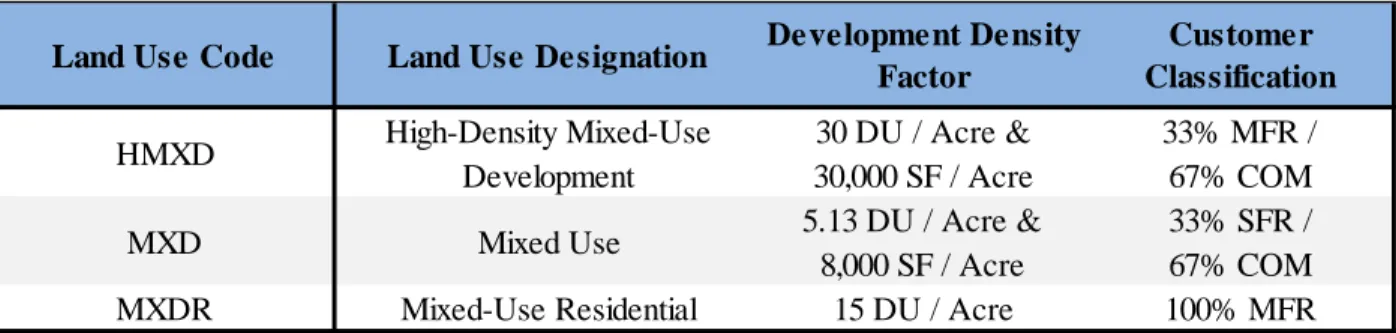
The breakdown of different assumptions for each mixed use category is included in Table 11. Interestingly, assumptions for the distribution of residential and nonresidential uses in the first two categories are the same except for the fact that the second category uses single family

residential (SFR) demand factors instead of multifamily residential (MFR) demand factors. Also, the ‘Mixed-Use Residential’ category follows the same pattern observed in other utility planning documents and simply applies the standard MFR demand factor to the entire property.

Table 11: Town of Cary 2009 Mixed Use Density Factors, and Classifications

Estimated demand for each mixed use category is calculated by multiplying the number of acres planned for that category by the customer classification percentage and development density factor and then applying the appropriate demand factor. Referring to Tables 8 and 9 above, the formula for estimating gallons of annual water use for a 10-acre HMXD development would be:

𝐴𝑛𝑛𝑢𝑎𝑙 𝐷𝑒𝑚𝑎𝑛𝑑 = (10 × 0.33 × 30 × 42.3) + (10 × 0.67 × 30,000 × 0.037) ≈ 11,625

In general, I think this ‘additive’ approach makes more sense than simply relying upon the demand factor for the underlying residential land use. It has the advantage of recognizing differences in water use between customer types and could be further refined as necessary to account for emerging patterns of development. Also, the fact that it is based on existing land use codes facilitates coordination between utilities and planning departments for municipalities within their service area. Another alternative approach would be to actually develop demand factors that specifically apply to mixed use developments.

HMXD High-Density Mixed-Use

Development

30 DU / Acre & 30,000 SF / Acre

33% MFR / 67% COM

MXD Mixed Use 5.13 DU / Acre &

8,000 SF / Acre

33% SFR / 67% COM

MXDR Mixed-Use Residential 15 DU / Acre 100% MFR

Land Use Code Land Use Designation Development Density Factor

(25)

21 | P a g e

Water Use in Selected Local Developments

Methodology

Given the wide variation in water use rates between different properties and locations, and the relative lack of information about the water use patterns of mixed use properties in particular, it is helpful to examine the actual characteristics and historical demands of mixed use

developments in OWASA’s service area. Toward that end, this section presents the results of interviews conducted with property managers at several sites in Chapel Hill and Carrboro along with analyses of historical water use data provided at the meter level by OWASA. A copy of the questionnaire that guided these interviews as well as a series of profiles summarizing water use at each property are included as Figures A.1 through A.5 in the Appendix. The overarching goal of this research was to capture information about the presence of various efficiency and

conservation measures in order to provide a point of comparison for the average annual demand assumptions presented in the previous sections. The properties included in this process were selected as examples of the types of developments that OWASA officials expect to become more prevalent in their service area going forward. Future studies could expand upon this research by attempting to survey a larger number of properties both inside OWASA’s service area, and in other local municipalities. Topics covered in the interviews include:

 Fixture sizes/types

 Metering/billing systems

 Mission statements, marketing collateral, and/or expressed ethos

 Behavioral programs targeting sustainability

 Maintenance staff size

 Known maintenance issues

 Management type

 Property ownership

 Building size and number of units

 Irrigation practices

 Land size and characteristics

 Amenities including pools and cooling towers

 Occupancy patterns

 Any additional water saving features

Since the properties included in this process were constructed at different times, the amount of meter data available for each development varies from nearly 5 years for Greenbridge to just over 2 years for 300 East Main. Additionally, it should be noted that certain data points acquired during the interviews may be rather imprecise. For example, occupancy data was reported only on an annual basis, and should likely be viewed as estimates rather than hard figures based on rent rolls or reviews of actual leases.

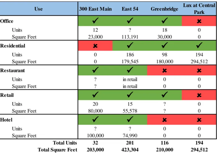
Mix of Uses

(26)

22 | P a g e

Greenbridge has recently installed a separate meter for the cooling tower in that property, so in the future it should be possible to differentiate cooling tower water from water drawn through the master meter.

Table 12: Survey Property Characteristics

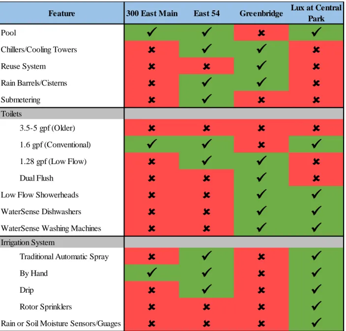
Fixtures & Amenities

During the interview process, property managers were asked to indicate whether or not their structures contained the water-related features included in Table 13 on the next page. Their responses point to many differences between the structures, but also mask certain facts that might help explain why a specific feature might be present in one property but not another. For example, since they are both infill developments with little to no greenspace, it would not make sense for either Greenbridge or 300 East Main to invest in an automatic irrigation system. Along similar lines, 300 East Main’s decision not to install WaterSense appliances is simply a reflection of the lack of residential units in the property, not a lack of effort to save water.

As a LEED Gold building, Greenbridge has taken the most extreme steps to conserve water. In fact, Greenbridge has installed all of the most efficient options for restroom fixtures, appliances, and irrigation included in the questionnaire. The Lux at Central Park, however, has nearly identical in-unit features with the exception of 1.28 gpf and dual flush toilets. East 54 has also received LEED recognition, with the entire development earning recognition through the pilot LEED-Neighborhood Development program, and the office portion receiving LEED-Platinum through the Core and Shell program. The fact that some properties have installed high-efficiency

Units ? ? 0 0

Square Feet 100,000 74,990 0 0

Total Units 32 201 116 194

(27)

23 | P a g e

features without seeking LEED certification may suggest an opportunity to supplement market pressures with other incentives in order to push new development toward higher water

conservation standards.

Table 13: Survey Property Features

Building Level Average Annual Demand

Average annual demand was calculated for each year in which both of the following conditions were met: (1) the property was operational for at least 10 months; and, (2) meter data was available for at least 10 months. All demand figures represent a combination of both indoor and outdoor demand, since metering was inconsistent across properties. If a property was operational or data was only available for 10 months in a given year, then an average monthly demand rate was used to produce implied annual demand. For example, meter data for the Lux at Central Park was only available for the first 10 months of 2016, so the annual demand calculated for that year

Feature 300 East Main East 54 Greenbridge Lux at Central



Toilets



WaterSense Dishwashers





WaterSense Washing Machines

(28)

24 | P a g e

is equal to the total actual demand for the first 10 months plus two times the average monthly demand in 2016. The reported average annual demand figure for the Lux at Central Park was then calculated by taking the average of actual and implied water demand figures for both 2015 and 2016.

A similar approach was used for average annual demand per dwelling unit (DU) in order to account for occupancy levels. Demand per DU was calculated as the total demand for each month divided by the estimated number of occupied DUs. Again, using the Lux at Central Park as an example, the questionnaire indicated that there was a 75 percent occupancy rate across 194 total units at the end of 2014. The calculated demand per DU for December 2014 is therefore equal to the actual volume of water reported by OWASA divided by 0.75 × 194 = 146 units. Average annual demand per DU was then calculated as the average of these monthly figures for each year of operation. That said, since the Lux at Central Park was only operational for 2

months in 2014, the reported average annual per DU and average annual demand figures exclude averages from that year. East 54 did not provide occupancy data, so a flat rate of 95 percent occupancy was assumed for the entire period. Since we do not know which DUs were occupied at any given point in time, it is not practicable to estimate the number of occupied square feet for each month. Average annual demand per square foot figures have therefore not been adjusted to account for occupancy.

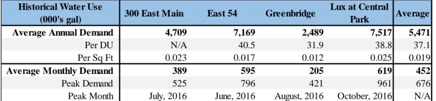
Table 14 below provides a summary of average water use for each of the surveyed properties. There are several patterns within this table worth noting. First, there is substantial variation across the water use rates for both per DU and per SF demands. Annual per DU demand ranges from a low of 31.9 kgpu for Greenbridge to 40.5 kgpu for East 54. This fact may be surprising given that both of these properties have received some level of LEED recognition, but the difference makes more sense considering the distribution of uses (Table 12). Indeed, residential uses account for approximately 86 percent of the total square footage at Greenbridge, but only around 42 percent of the total square footage at East 54. This means that the per DU rate for East 54 is skewed upward by the presence of over 243,000 SF of nonresidential units, thus illustrating one of the drawbacks of using per DU demand factors for mixed use properties. Another pattern worth noting is that both Greenbridge and East 54 display a substantially lower per SF water use rate than the two non-LEED properties. Finally, it is interesting that all four properties had their highest monthly use in 2016, although two properties (300 East Main, and The Lux at Central Park) only had two or three years of available data.

Table 14: Survey Property Average Demand

Table 15 provides a comparison between the average annual rates observed for the four survey properties and the average rates referenced earlier in this report. Note that the value of this

Historical Water Use

(000's gal) 300 East Main East 54 Greenbridge

Lux at Central

Park Average

Average Annual Demand 4,709 7,169 2,489 7,517 5,471

Per DU N/A 40.5 31.9 38.8 37.1

Per Sq Ft 0.023 0.017 0.012 0.025 0.019

Average Monthly Demand 389 595 205 619 452

Peak Demand 525 796 421 961 676

Talley_Trey.pdf

Anticipating Mixed Use Water Demand:

Chapel Hill & Carrboro, NC

Anticipating Mixed Use Water Demand:

Chapel Hill & Carrboro, NC

Department of City & Regional Planning

UNC Chapel Hill

Trey Talley

Table of Contents

Acronyms

Introduction

Factors Affecting Mixed Use Water Demand

Anticipating Mixed Use Water Demand in OWASA’s Service Area

Water Use in Selected Local Developments



































































































































