A Robust Dispersion Control Chart Based on M-estimate

Vol. 2, No. 4, pp 297-307 Winter 2009

A Robust Dispersion Control Chart Based on M-estimate

Faculty of Industrial Engineering, K. N. Toosi University of Technology, Tehran, Iran 1 _{[email protected],} 2 _{[email protected],} 3 _{[email protected]}

ABSTRACT

Process control charts are proven techniques for improving quality. Specifying the control limits is the most important step in designing a control chart. The presence of outliers may extremely affect the estimates of parameters using classical methods. Robust estimators which are not affected by outliers or the small departures from the model assumptions are applied in this paper to specify the control limits. All the robust estimators of dispersion which have been proposed during the last decade are evaluated and their performance in control charting is compared. The results indicate that the M-estimate is a better estimator of dispersion in the presence of outliers. We show that when the M-estimate with a bisquare ρ-function is used to estimate the dispersion, the S control chart has the best performance among all estimators.

Keywords: Statistical process control, S chart, Robust statistics, M-estimate.

1. INTRODUCTION

Process control charts are proven techniques for improving quality and productivity. A typical approach is to collect rational subgroups of reasonable sample sizes and then to construct control charts. Dispersion control charts, such as S chart, are the main focus of this research. In S control chart, if the standard deviation of a subgroup falls beyond the limits, it is an indication that the process variability is out of control.

Specifying the control limits is the most important step in designing a control chart. Improper estimation of the process dispersion which results in narrower or wider limits can increase the committed probability of type I error or the probability of type II error. When the limits are narrow the risk of a point falling beyond the limits, indicating an out of control when in fact the process is in control, increases. When the limits are wider the risk of a point falling between the limits, while the process is really out of control, increases. The presence of inliers or outliers cause an increase in risk of type I or risk of type II, respectively. The case of having only outliers is considered here. The presence of outliers may extremely affect the estimate of the parameters using classical methods. One approach to reduce the effect of outliers is to use an adaptive trimmer that iteratively deletes subsamples whose standard deviations fall outside the control limits. Once, the limits are recomputed the procedure of eliminating subsamples with standard deviations outside the control limits is repeated. This procedure has some drawbacks one which is addressed here.

When there are several outliers, average of standard deviations of subgroups may increase vastly and the 3-sigma distance will be inflated. Hence, the outliers remain unnoticed. This drawback will be examined in simulation study later in the paper.

Robust estimation is a new approach to estimate parameters. Such an approach provides ways to emulate classical methods, while not being unduly affected by outliers or other small departures from model assumptions. Classical methods are efficient in the absence of outliers, i.e., when model assumptions are true. For instance, when the data are from normal distribution, classical estimates are in some sense optimal when the data are normally distributed. But, they are suboptimal when the distribution of the data differs slightly from the assumed model. On the other hand, robust estimates maintain approximately optimal performance, not only under the assumed model, but also under small perturbations.

Application of robust statistics in statistical process control has increased in the past decade. The role of robust estimation has been well stated by Rocke (1989), who observed that:

• Statistics that are used to calculate the control limits should be robust against outliers. • Statistics that are indicated in the control chart should be sensitive to outliers.

Langenberg and Iglewicz (1986) proposed trimmed mean of subgroup ranges, Rocke (1989) used interquartile range (IQR) and Tatum (1997) recommended the modified bisquare A-estimator to estimate the standard deviation of the population. In addition, Mast and Roes (2004) used A-estimator for individual control chart and Omar (2008) suggested mean of subgroups median absolute deviations (MAD) as a dispersion estimator.

In this article the M-estimate with a bisquare ρ-function is suggested for estimating the process dispersion and determining the control limits for S charts. In section 2, the suggested estimator is introduced and the robustness of estimators is discussed in Section 3. Section 4 deals with mean squared error (MSE) which is used to evaluate the efficiency of the estimators. In section 5 the performance of control charts are compared by means of mean square deviation (MSD).

Simulated data from mixture of standard normal distribution and normal distribution with arbitrary parameters are generated, and the efficiency of estimators and the performance of control charts are assessed.

2. THE PROPOSED METHOD

M-estimates as proposed by Huber (1981) are the generalized forms of maximum likelihood estimates (MLEs). M-estimate is the solution of the equation (1)

(

)

1

ˆ _{arg min ,}

n i i

x θ

θ ρ θ

=

= ⎛_⎜ ⎞_⎟

⎝

∑

where ρ is a function with certain properties. Given f is a density function andρ = −logf , then ˆ

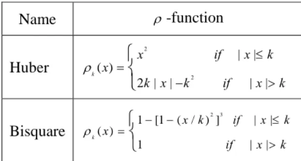
θ will be interpreted as the maximum likelihood estimator (MLE) of the parameter of distribution. There are several ρ-functions each of which has special properties. Two popular ρ-functions are Huber and bisquare (Maronna et al., 2006). These functions are shown in Table 1. The value of k is

chosen to ensure a high efficiency for the normal distribution. When the data are drawn from a normal distribution, the value of k should be determined in such a way that the M-estimator has a variance close to the variance of the optimal classical estimator.

The proposed ρ-function is a bisquare with k=1. The M-estimate for dispersion is also called the M-estimate of scale.

The M-estimate of scale is the solution of equation (2)

0 1 ˆ 1 ˆ n i i x n µ ρ δ σ = − = ⎛ ⎞ ⎜ ⎟ ⎝ ⎠

∑

where µˆ₀ is the primary mean estimate and δ is a positive constant.

There are several methods to compute M-estimates, such as Newton-Raphson, iterative pseudo-observations and iterative reweighting algorithm, Maronna et al. (2006). Among these methods, the third algorithm, described in Appendix, is used. Let W x( )=ρ( ) /x x2, where ρ is a ρ-function in M-estimation.

Table 1. Huber and bisquare ρ-functions

Name ρ-function

Huber

2

2

| | ( )

2 | | | |

k

x if x k

x

k x k if x k

ρ = ≤

− > ⎧ ⎨ ⎩ Bisquare 2 3

1 [1 ( / ) ] | | ( )

1 | | k

x k if x k

x

if x k

ρ = − − ≤

>

⎧ ⎨ ⎩

The preference for this method is that when W x( ) is bounded, even, continuous and non-increasing forx>0, then this method converges to the solution of equation (2) while, there is no guarantee for the other methods to converge to this solution (Maronna et al., 2006).

M-estimates of location and scale can be determined simultaneously or separately. Each method has its own properties. In general, separate estimation is more robust than simultaneous estimation. Simultaneous estimation is more useful in multivariate analysis (Maronna et al., 2006).

3. ROBUSTNESS OF ESTIMATES

Maronna et al. (2006) described three measures of robustness: Influence Function, Breakdown Point, and Maximum Bias. Influence function deals with small proportion of outliers, while breakdown point deals with large proportions. In addition, maximum bias clearly shows maximum bias of estimate for different proportions of outliers. Among these measurements, the breakdown point is more applicable than the others. However, Tatum (1997) defined breakdown bound of the control charts as b*= p mn/ , where n is the sample size, m is number of subgroups and p is the

largest number of individual observations that could be manipulated while still leaving the estimate bounded. This definition is roughly similar to the definition of the breakdown point which Maronna et al. (2006) have demonstrated. It is clear that there must be more typical than atypical individual data and so b*≤0.5.

Manipulation of only one observation can drive the estimates beyond any given bound. So it is clear that the breakdown bound of the average subgroup ranges and the average subgroup standard deviations are zero. One of the useful estimators is α-trimmed mean of data which discards α proportion of largest and smallest data and generally its breakdown point is equal to α (Maronna et al., 2006).

Langenberg and Iglewicz (1986) proposed 25% trimmed mean of the subgroup ranges to estimate σ. Suppose that m=20 and n=5, therefore this estimator trims the largest five and the smallest five subsample ranges. If one observation in each of the six subsamples is manipulated, then this estimate can be forced beyond any given bound so that the breakdown bound of this estimate becomesb* =p mn/ =5 /(20 5)× =0.05. Hence, breakdown bound for α-trimmed mean of subgroup ranges is

* _{/ /}

b =mα mn=α n (3)

Another estimate can be considered by using IQR. Rocke (1989) suggested the average of IQR’s subsample which is defined by

( ) ( ) 1

1 IQR

m

b j a j j

x x

m =

=

∑

where x_{( )b j} is the bth order statistic in the jth subgroup and a=

[

]

n= IQR is calculated by the difference between the second largest and the second smallest data. As a result, two outliers in one subgroup can disturb σˆ beyond any given bound. So breakdown bound for the average of IQR’s is 1/mn for n=4, 5, 6, 7 and 2 /mn for n=8, 9,10,11. For example, if m=20 and n=5 then b*=0.01. Rocke (1989) also proposed 25% trimmed mean of IQR’s subsample which its breakdown bound for n=4, 5, 6, 7 is *

2 / 4 1/

b = ⎡_⎣m ⎤_⎦+ mn.

estimator is another alternative as a dispersion robust estimator. Tatum (1997) used modified A-estimator and claimed that its breakdown bound is roughly 25%.

Maronna et al. (2006) proved that breakdown point for M-scale can be defined by δ in Equation (2) and that is min( ,1δ −δ). Thus when δ =0.5 is chosen, then b* =0.5 which is more desirable. Omar (2008) proposed mean of subgroups’ median absolute deviations to estimate dispersion of process. Although its breakdown point is equal to 0.5, its breakdown bound in control chart is much smaller. If m=20 and n=5, its breakdown bound is 0.02. Because three atypical observations in one subgroup can drive the estimation of process dispersion beyond any given bound. In addition, its efficiency under iid normal case is 37% which is not acceptable.

Breakdown bound explains robustness of an estimate and it doesn’t present anything useful about the bias or efficiency of an estimator. For instance, breakdown point of median as a mean estimator

is 0.5 while its efficiency in a case of iid normal is too low. Its bias is not so low in presence of outliers. In the next section the simulated data are used to measure and assess the aptness of the estimators.

4. MEASURING ESTIMATORS’ EFFCIENCY

In this section effort is made to find an estimator which estimates well, both in presence and absence of outliers. One thousand simulation runs of 20 subgroups each of size 5 were performed to generate data. The generated data have distribution from the mixture of standard normal and normal distribution with different parameters. The process dispersion is estimated by both classical and robust methods. The MSE for dispersion is calculated by

(

)

1000

2

1

1

ˆ MSE

1000 i i

σ σ σ

=

=

∑

where σ is the standard deviation of the process and ˆσ_i stands for the dispersion estimation in ith simulation run. The MSE for the following statistics which are used to estimate dispersion are computed and compared using the same simulated data.

1-S : The average of the subgroups’ standard deviations (Code S) 2- R : The average of the subgroups’ ranges (Code R)

3-AdaptiveS : The average of subgroups’ standard deviations that are within the control limits (Code aS)

4-AdaptiveR: The average of the subgroups’ ranges that are within the control limits (Code aR)

5-IQR: The average of the subgroups’ IQRs (Code IQR) 6-The 25% trimmed mean of the subgroups’ IQRs (Code IQRT) 7-The modified bisquare A-estimator with c=10(Code A10) 8-The modified bisquare A-estimator with c=7 (Code A7)

9-The simultaneous M-estimates of the location and the dispersion with bisquare ρ-function and 1

k= when the dispersion is estimated and k=3.44 when the location is estimated (Code SMD). 10-The M-scale with bisquare ρ-function and k=1 (Code MS)

11-The 25% trimmed mean of the subgroups’ ranges (Code RT)

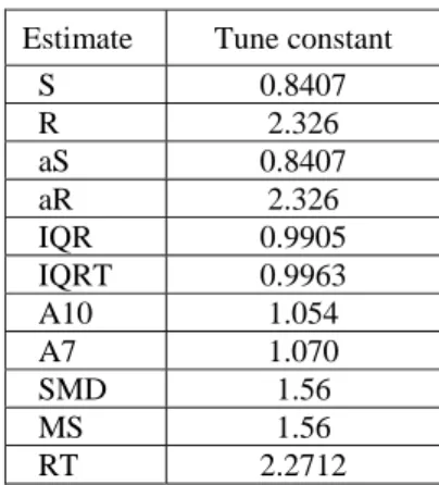
To provide an unbiased estimator of σ for the iid Normal case, the value provided by each of the eleven statistics must be divided by a normalizing factor. The factor for S, R, aS and aR are provided in Grant and Leavenworth (1996) and for codes IQR, IQRT and RT, they are obtained by 10000 simulation runs of 20 subgroups of size 5 using Matlab-software. The factors for A10 and A7 are computed by Tatum (1997) and finally the factors for SMD and MS are numerically calculated by Maronna et al. (2006). The dividing factors for estimating the process dispersion from different statistics are provided in Table 2.

Table 2. Tune constants for dispersion estimators

Estimate Tune constant

S 0.8407

R 2.326

aS 0.8407

aR 2.326

IQR 0.9905 IQRT 0.9963 A10 1.054

A7 1.070

SMD 1.56

MS 1.56

RT 2.2712

The estimators are compared based on three types of simulations:

Simulation type 1: generating mixed data from standard normal distribution with probability1-ε, and a normal distribution with mean a and standard deviation c, where

0.05, 0.10, 0.15, 0.20, 0.25

ε = , 0,1,..., 9a= and c=1, 2,..., 5. The distribution of data can be defined as

(0,1) P 1 ( , ) P

N N a c

ε ε = − =

⎧ ⎨

⎩ (6)

Simulation type 2: generating mixed data from normal distributions defined as the following

(0,1) P 1 ( , ) P / 2 ( , ) P / 2

N N a c N a c

ε ε ε = −

+ =

− =

⎧ ⎪ ⎨

⎪⎩ (7)

Where the values for ε , a and c are same as defined for simulation type 1.

Simulation type 3: generating mixed data from standard normal distribution, with the exception of one subgroup which is from N(0, )c where c=1, 2,..., 5.

The results to be presented are based on 1000 simulation runs for each level of change in a c, and ε for the three types of simulations.

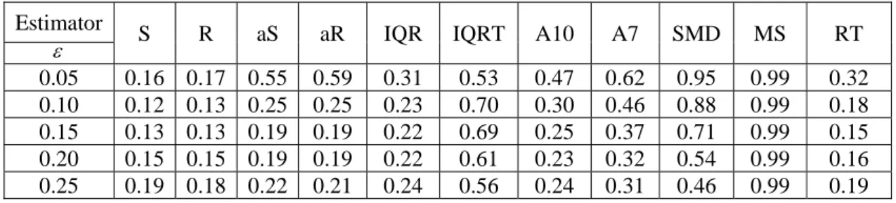
The efficiency of each estimator in estimating the process dispersion is measured by the average of relative mean square error (ARMSE) with respect to

ε

9 5

,

0 1 ,

Best MSE 1

ARMSE=

10 5 MSE

a c

a= c= a c

×

⎛ ⎞

⎜ ⎟

⎝ ⎠

Where MSEa,c stands for the MSE of the estimator when atypical data have normal distribution with

mean a and standard deviation c. And Best MSEa,c is the lowest MSE among estimators when

atypical data have normal distribution with mean a and standard deviation c. In addition it is clear that the estimator with the largest ARMSE is preferred. The maximum value for ARMSE is one.

Tables 3, 4, and 5 show ARMSE for simulation types 1, 2 and 3 for the eleven dispersion estimators. These tables illustrate that estimation based on MS is much better than the others. When proportion of outliers is low, the SMD is a good estimator. The third reasonable estimator, which is better than aS, aR, etc, is A7.

Fore more illustrative comparison of the estimators, control charts are used in the next section.

Table 3. ARMSE for dispersion estimators in Simulation type 1

Estimator

S R aS aR IQR IQRT A10 A7 SMD MS RT

ε

0.05 0.16 0.17 0.55 0.59 0.31 0.53 0.47 0.62 0.95 0.99 0.32 0.10 0.12 0.13 0.25 0.25 0.23 0.70 0.30 0.46 0.88 0.99 0.18 0.15 0.13 0.13 0.19 0.19 0.22 0.69 0.25 0.37 0.71 0.99 0.15 0.20 0.15 0.15 0.19 0.19 0.22 0.61 0.23 0.32 0.54 0.99 0.16 0.25 0.19 0.18 0.22 0.21 0.24 0.56 0.24 0.31 0.46 0.99 0.19

Table 4. ARMSE for dispersion estimators in Simulation type 2

Estimator

S R aS aR IQR IQRT A10 A7 SMD MS RT

ε

0.05 0.16 0.17 0.54 0.57 0.31 0.54 0.48 0.63 0.95 0.99 0.32 0.10 0.12 0.13 0.25 0.26 0.23 0.71 0.30 0.46 0.88 0.99 0.18 0.15 0.13 0.13 0.19 0.19 0.22 0.69 0.25 0.37 0.70 0.99 0.15 0.20 0.15 0.15 0.19 0.19 0.22 0.61 0.23 0.32 0.54 0.99 0.16 0.25 0.19 0.18 0.22 0.21 0.24 0.56 0.24 0.31 0.46 0.99 0.19

Table 5. ARMSE for dispersion estimators in Simulation type 3

Estimator S R aS aR IQR IQRT A10 A7 SMD MS RT ARMSE 0.30 0.31 0.30 0.32 0.59 0.82 0.39 0.44 0.82 0.86 0.28

5. CONTROL CHARTS’ PERFORMANCE

This section deals with control charts’ performance which is meant to show how good control charts are in detecting the positive signals. Although the most universal and applicable way to measure performance of control charts is the use of average run length (ARL), in this article the MSD is used to compare the performance of dispersion control charts. The MSD was applied by Tatum (1997) in a similar work to compare the performance of estimators.

The standard deviations applied to define the control limits are the estimators described in section 4. The data used in section 4 to evaluate the estimators are also applied here to define the control limits.

Tatum (1997) described the MSD for the dispersion control chart as

[

]

1000

2

1 1

MSD( ) ( , ) ( , ) 1000 i

J S J i S σ i

=

=

∑

where J shows the method of dispersion estimation, J =1, 2,...,11, S J i( , ) is the number of positive signals in the control charts using the Jth estimator and S( , )σ i is the number of positive signals in the dispersion control charts when σ is assumed to be known.

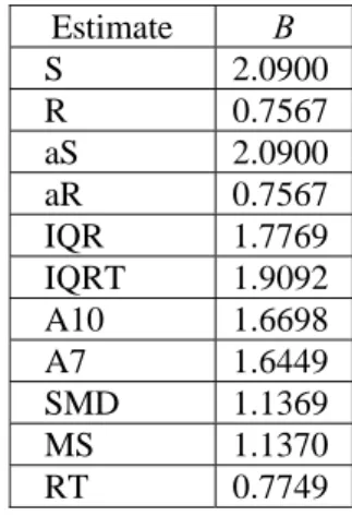
In the first step the control limits were modified such that the average false alarm rates under the normality assumption were equal when different estimators were used for dispersion. When σ was assumed to be known, an upper control limit equal to UCL=1.76σ yields a rate of 3.86% false alarms. The rate was obtained from 100000 simulation runs under normality assumption with known mean and variance. The values for B in UCL=Bσˆ were acquired from the same simulated data for IQR, IQRT, A10, A7, SMD, MS and RT. The values for S, R, aS and aR were taken from Grant and Leavenworth (1996). Table 6 provides the values for B.

Table 6. The values of B in UCL=Bσˆ for dispersion estimators Estimate B

S 2.0900 R 0.7567 aS 2.0900 aR 0.7567 IQR 1.7769 IQRT 1.9092 A10 1.6698 A7 1.6449 SMD 1.1369 MS 1.1370 RT 0.7749

Similar to the ARMSE which was used to introduce the best estimator, the average of relative mean square deviation (ARMSD) is applied to measure the performance of a control chart under different estimators for dispersion. The ARMSD is defined as:

9 5

,

0 1 ,

Best MSD 1

ARMSD=

10 5 MSD

a c

a= c= a c

⎛ ⎞

⎜ ⎟

⎜ ⎟

×

∑∑

where MSDa,c stands for the MSD of the control chart when atypical data have normal distribution

with mean a and standard deviation c. And Best MSDa,c is the lowest MSD among control charts

when atypical data have normal distribution with mean a and standard deviation c.

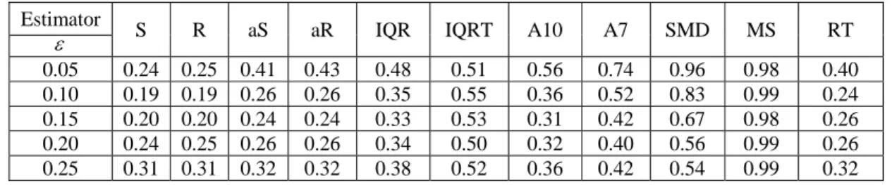
Tables 7, 8 and 9 show the ARMSD for dispersion control charts for Simulation types 1, 2 and 3. It is clear that dispersion control charts based on MS have the largest ARMSD and the best performance. The SMD had higher ARMSD when the value of ε is small. Hence MS is the best estimator for dispersion.

Table 7. ARMSD for dispersion control charts in Simulation type 1

Estimator

S R aS aR IQR IQRT A10 A7 SMD MS RT ε

0.05 0.25 0.25 0.42 0.44 0.48 0.51 0.57 0.76 0.95 0.98 0.41 0.10 0.19 0.19 0.25 0.26 0.35 0.55 0.36 0.52 0.84 0.98 0.25 0.15 0.20 0.20 0.23 0.23 0.33 0.53 0.31 0.41 0.67 0.98 0.23 0.20 0.25 0.25 0.27 0.27 0.34 0.51 0.32 0.39 0.56 0.99 0.26 0.25 0.31 0.31 0.32 0.32 0.39 0.52 0.36 0.42 0.54 0.99 0.32

Table 8. ARMSD for dispersion control charts in Simulation type 2

Estimator

S R aS aR IQR IQRT A10 A7 SMD MS RT ε

0.05 0.24 0.25 0.41 0.43 0.48 0.51 0.56 0.74 0.96 0.98 0.40 0.10 0.19 0.19 0.26 0.26 0.35 0.55 0.36 0.52 0.83 0.99 0.24 0.15 0.20 0.20 0.24 0.24 0.33 0.53 0.31 0.42 0.67 0.98 0.26 0.20 0.24 0.25 0.26 0.26 0.34 0.50 0.32 0.40 0.56 0.99 0.26 0.25 0.31 0.31 0.32 0.32 0.38 0.52 0.36 0.42 0.54 0.99 0.32

Table 9. ARMSD for dispersion control charts in Simulation type 3

Estimator S R aS aR IQR IQRT A10 A7 SMD MS RT

ARMSD 0.46 0.46 0.44 0.45 0.82 0.79 0.56 0.65 0.90 0.92 0.43

6. CONCLUSIONS AND RECOMMENDATIONS

This article presents two essential points. The first is that the classical estimators have some drawbacks when the true model deviates from the assumed distribution.

The second is that using robust estimators yield better estimates than classical estimates in presence of outliers for process dispersion. Furthermore, when no outlier exists among the data, the robust estimators perform the same as the classical estimators.

The M-estimator with bisquare ρ-function and k=1 suggested in this article for control charting performs better than other estimators for dispersion.

The robust estimators may behave differently under non-normal assumptions. This could be investigated in a separate research effort.

Acknowledgements

We thank anonymous referees for their helpful comments.

Appendix: Numerical Computation of M-estimate of scale

First, a good start point should be calculated as initial estimation of location and dispersion. Sample median and normalized median absolute deviation (MADN) can be used in this case. MADN is calculated as

Med (|x-Med(x)|) MADN

0.6745

= (A-1)

Now, the weight function is defined as

ˆ ˆ

w W

µ

σ

⎛ ⎞

= ⎜_⎝x ⎟_⎠ (A-2)

where W is as defined in (A-3).

2

( ) / 0 ( )

(0) 0

x x if x

W x

if x

ρ ρ

≠ =

′′ =

⎧ ⎨

⎩ (A-3)

where ρ( )x is theρ-function. Then

σ

2 1

1

ˆ ˆ

n

new old i

i wr n

σ

σ

δ

=

∑

where ˆ

ˆ

i i

old x

r

µ

σ

= . Moreover,µˆ is constant and ˆσ is updated in each iteration to estimate M-scale. Also, both µˆ and σˆ are updated to calculate simultaneous M-estimation.

Stopping condition is |σˆ_k+1/σˆ_k − <1 | ε.

REFERENCES

[1] Grant R., Leavenworth R. (1996), Statistical quality control; 7th edition, McGraw-Hill; New York. [2] Huber P.J. (1981), Robust statistics; Wiley; New York.

[3] Janace G.J., Meikle S.E. (1997), Control charts based on medians; The Statistician 46(1); 19-31. [4] Langenberg P., Iglewicz B. (1986), Trimmed mean X and R charts; Journal of Quality Technology

18; 152-161.

[5] Maronna R.A., Martin R.D., Yohai V.J. (2006), Robust statistics, Theory and methods; Wiley; New York.

[6] Mast J., Roes C.B. (2004), Robust individual charts for exploratory analysis; Quality Engineering 16(3); 407-421.

[7] Omar Moustafa (2008), A simple robust control chart based on MAD; Journal of Mathematics and Statistics 4(2); 102-107.

[8] Rocke D.M. (1989), Robust control charts; Thechnometrics 31(2); 173-184.

[9] Tatum L.G. (1997), Robust estimation of the process standard deviation for control charts; Thechnometrics 39(2), 127-141.