The Effect of Gauge Measurement Capability and Dependency Measure of Process Variables on the MCp

Vol. 4, No. 1, pp 59-76 Spring 2010

The Effect of Gauge Measurement Capability and Dependency Measure

of Process Variables on the MC

p

Davood Shishebori 1∗, Ali Zeinal Hamadani 2

Department of Industrial Engineering; Isfahan University of Technology; Iran; 1 _{[email protected],} 2 _{[email protected]}

ABSTRACT

It has been proved that process capability indices provide very efficient measures of the capability of processes from many different perspectives. These indices have been widely used in the manufacturing industry for measuring process reproduction capability according to manufacturing specifications. In the past few years, univariate capability indices have been introduced and used to characterize process performance, but are comparatively neglected for multivariate processes where multiple dependent characteristics are involved in quality measurement. Also, most of researches related to process capability indices have assumed no gauge measurement errors. Unfortunately, such an assumption does not reflect real situations accurately even with highly sophisticated advanced measuring instruments. Conclusions drawn from process capability analysis are hence unreliable. In this paper, we consider the effect of process variables correlation coefficient on the multivariate process capability index (MCp) for

different gauge measurement capabilities. Also, with respect to correlation coefficient and measurement capability we investigate the statistical properties of the estimated MCp. The

results indicate that gauge measurement capability has an important role in determining process capability. This factor would increase the effect of correlation coefficient on estimating the process capability, such that for different gauge measurement capabilities, correlation coefficients will change the results of estimating and testing the process capability.

Keywords: Capability analysis, Correlation coefficient, Critical value, Hypothesis testing,

Multivariateprocess, Gauge measurement errors. 1. INTRODUCTION

In manufacturing industry, there is growing interest in quantitative measures of industrial processes variation. One of the measuring tools most frequently used to measure the capability of a manufacturing process is process capability indices, designed to quantify the relation between the actual performance of the process and its specified requirements. These indices have received much interest in statistical literature during recent years (Vannman and Hubele , 2003). It has been proved that process capability indices provide very efficient measures of the capability of processes from many different perspectives (Chang and Wu, 2008). These capability indices, quantifying process potential and performance, are important for any successful quality improvement activity and

quality program implementation.

∗_{Corresponding Author}

Capability indices, Cp, Cpk, Cpm, and Cpmk, have been proposed in the manufacturing and service

industries providing numerical measures on whether a process is capable of reproducing items within the specification limits preset in the factory. A large number of papers have dealt with the statistical properties and the estimation of these univariate indices. Kotz and Johnson (2002) provided a compact survey and commented on some 170 publications on process capability indices during the years 1992 to 2000. Also Pearn and Kotz (2006) provided a comprehensive survey on process capability indices during the beginning of introducing these indices up to late 2005.

One interesting fact about the characteristic measuring in a process is that the inevitable variations in process measurements come from two sources: the manufacturing process and the gauge. Gauge capability reflects the gauge's precision, or lack of variation, but is not the same as calibration which assures the gauge's accuracy. As it has been emphasized in numerous occasions, process capability measures the ability of a process to meet reassigned specifications.

Most of research papers related to capability measure have assumed no gauge measurement errors (Pearn and Liao, 2005). Unfortunately, such an assumption does not reflect real situations accurately even with highly sophisticated advanced measuring instruments. Montgomery and Runger (1993) pointed out that the quality of data on the process characteristics relies very much on the gauge. Pearn et al. (2007) mentioned that any variation in the measurement process has a direct impact on the ability to make sound judgment about the manufacturing process. An inaccurate measurement system can thwart all the benefits of improvement endeavors resulting in poor quality. On the other hand, improving the gauge measurements and employing properly trained operators can reduce the measurement errors. However, the reality is that no measurement is free from error or uncertainty even if it is carried out with the aid of highly sophisticated and precise measuring instruments. Some research has been done for the case of univariate process capability while considering the measurement error in particular states. Pearn and Kotz (2006) provided a compact survey on pervious researches capability indices with gauge measurement errors during the beginning of introducing these indices up to late 2005.

Another point that is crucial in process capability indices is the bulk of the studies associated with analyzing the quality and efficiency of a process due to a single quality specification; but in modern manufacturing environments where complex processes require monitoring, the possibility of simultaneously monitoring and controlling two or more quality features is rapidly gaining importance. So, our studies on capability indices can not be restricted to the univariate domain. For this reason, multivariate methods for assessing process capability are proposed.

Chan et al.(1991), Taamet al.(1993), Pearnet al.(1992), Chen(1994), Karl et al.(1994), Shahriari

et al.(1995), Boyles(1996), Wang and Du (2000), Wang et al. (2000), and others have developed

and presented multivariate capability indices for assessing capability. Wang and Chen (1998) and

Wang and Du (2000) proposed multivariate extensions for Cp, Cpk, Cpm, and Cpmk based on the

principal component analysis, which transforms numbers of original related measurement variables into a set of uncorrected linear functions. A comparison of three novel multivariate methodologies

for assessing capability is illustrated in Wang et al.(2000). Although some multivariate capability

indices have been studied, and an extensive study has been done for the case of univariate process capability while considering the measurement error, there is a real need for considering this effect on the multivariate quality characteristics as there no study conducted in this regard.

In this paper we focus on the common capability index, MCp in multivariate state and consider the

measurement capabilities; in other words, we try to answer the question if there is a sound effect of

correlation coefficient on the estimation of MCp, when the measurement error increases.

2. MULTIVARITAL PROCESS CAPABILITY IN PRESENCE OF GAUGE MEASUREMENT ERRORS

The multivariate capability index MCp is defined as (Taam et al.(1993)):

1 2 2 / 1 2 / 2

9973 . 0 ,

1 _{( ) | | [ ( 1)]}

) (mod

)] ( ) ( ) [(

) (mod

−

− _{− ≤} = _{∑ Γ +}

∑ ′ − =

v v

v

p Vol ified tolerance region

q k X

X Vol

region tolerance ified

Vol MC

πχ μ

μ (1)

Where k(q) is the 99.73th percentile of the

_χ

2 _{distribution with v degrees of freedom or the}

dimension of variables; μ is the mean vector and

∑

represents the variance–covariance matrix of

X; ∑ is the determinant of

∑

and Γ

()

. is the gamma function; Vol (modified tolerance region) is

the largest ellipsoid centered at the target completely within the original tolerance region; and

)] q ( k ) X ( ) X [(

vol _{−μ ′ ∑}−1 _{−μ ≤ indicates a scaled 99.73% process elliptical region.}

Gauge repeatability and reproducibility (GR&R) studies focus on quantifying the measurement errors. Suppose that in the multivariate case, the measurement errors are described by a random

variable M ~ Normal (

μ

_Me

,

∑

_Me), where

μ

_Me = 0, is the mean vector, and

∑

_Meis the Variance

covariance matrix of the measurement error. So, based on the definition of Montgomery and Runger (1993), the gauge capability for the multivariate case is defined by:

) (mod

)] 1 ( [ | | ) (

region) tolerance ed

Vol(modifi

)] ( ) (

)

[( 1 2,0.9973 /2 1/2 2 1

region tolerance ified

Vol q

k X

X

Vol Me Me Me v v Me v

M ₌ −μ ′∑− −μ ≤ ₌ πχ ∑ Γ + −

λ (2)

Where ∑_Me is the determinant of

∑

_Me and and

λ

M is the gauge capability index for the

multivariate case. For the measurement system to be deemed acceptable, the variability in the measurements due to the measurement system must be less than a predetermined percentage of the engineering tolerance. So based on the recommendations, some guidelines for gauge acceptance are offered (Montgomery, 1996).

Considering the process capability in the measurement error system, we assume that the

observations X have a multivariate normal distribution Nv(μ,

∑

) and show the relevant quality

characteristic of a manufacturing process. Because of measurement errors, the observed variable Y

~ Nv(μY =μ, ∑Y =∑+∑Me) is measured by the assumption that X and Me are stochastically

independent, instead of measuring the true variable X. The empirical process capability index

(MCY_p) is obtained after substituting ∑_Y for

∑

, so the multivariate capability index

MC

Y_p is

defined as:

1 2 2 / 1 2 / 2

9973 . 0 ,

1 _{( ) | | [ ( 1)]}

) (mod

)] ( ) (

) [(

) (mod

−

− _{− ≤} = _{∑ Γ +}

∑ ′ − =

v Y

v v

Y Y

p Vol ified tolerance region

q k X

X Vol

region tolerance ified

Vol MC

πχ μ

It is easy to show that the relationship between the true process MCp and the empirical process

capability Y

p

MC is given as (Shishebori and Hamadani, 2008):

| | | | | | 2 ) ( Me Y Me Y p M p Y p MC MC MC ∑ − ∑ −∑ ∑ + =

λ (4)

Since the variation of data we observe is larger than that of the original data, the denominator of the

index MCp becomes larger and we will underestimate the true capability of the process.

3. ESTIMATION OF MCp IN PRESENCE OF GAUGE MEASUREMENT ERRORS

An estimator of MCp can be expressed as

1 2 2 / 1 2 / 2 9973 . 0

, ) | | [ ( 1)]

( ) (mod ) % 73 . 99 .( ) (mod ˆ − + Γ = = v v v p S region tolerance ified Vol region process estimated Vol region tolerance ified Vol C M πχ

Where S is the sample variance-covariance matrix from process and |S| is the determinant of S.

p C

Mˆ is a biased estimator of MCp multiplied by bv given as:

] 2 / 1 ) ( 2 / 1 [ )] 1 ( 2 / 1 [ ) 1 2

( /2

− − Γ − Γ − = v n n n b v v

We get an unbiased estimation of MCpas M~C_p =b_vMˆC_p.Pearn et al. (2007) showed that M~C_p is

the UMVUE (Uniformly Minimum Variance Unbiased Estimator) of MCp.

With respect to gauge measurement capability and using the estimators, SY, SMe and MˆC_p for the

parameters∑_Y,

∑

_Me and MCp, the biased estimator of MCp is given as:

1 2 2 / 1 2 / 2 9973 . 0 , 1 2 2 / 1 2 / 2 9973 . 0

, ( ) | | [ ( 1)]

) (mod )] 1 ( [ | | ) ( ) (mod ˆ −

− = _{+ Γ +}

+ Γ = v Me v v v Y v v Y p S S region tolerance ified Vol S region tolerance ified Vol C M πχ

πχ (5)

Where SY is the sample variance-covariance matrix and |SY| is the determinant of SY.

So the relationship between the estimators of the true process MCp and the empirical process

capability MCY_p is given as:

| | | | | | 2 | | | | | |

2 ₍~ ~ ₎

~ ~ ) ˆ ˆ ( ˆ ˆ Me Y Me Y Me Y Me Y S S S S p M p Y p S S S S p M p Y p C M C M C M or C M C M C M − − − − = ₊ + = λ λ (6) Illustration Example

It is assumed a bivariate quality control involving joint control of the length (L) and width (W) of a plastic product from a multivariate normality (both quality characteristics/ dimensions have the same unit of measure). Twenty five observations were collected from a plastic production line using

the same gauging device. The specification limits for L and W were set at (112.7, 241.3) and (32.7,

73.3), respectively. The center of the specifications was T

0

μ

= [177, 53]. The sample mean vector

and sample covariance matrix were

⎥ ⎦ ⎤ ⎢

⎣ ⎡ = =

6594 . 44 3308 . 85

3308 . 85 8347 . 348 ,

] 32 . 52 , 2 . 177

[ Y

T _S

X

Using 2

9973 . 0 , 2

χ

= 11.829 and |SY| = 8297.4, then we obtain the practical estimated value of process

capability index as:

2114 . 1 2

/ 1 | | ) 2

9973 . 0 , 2 (

] 2 / ) 7 . 32 3 . 73 [( ] 2 / ) 7 . 112 3 . 241 [(

ˆ ₌

×

− ×

− ×

=

Y S p

C M Y

χ π π

and ~ Y =(11/12)×(1.2114) =1.1104

p C

M .

This value is calculated by ignoring the gauge measurement capability. Now by considering the gauge measurement error for the data, and with respect to the independence of measuring instruments for two variables, we assume that the variance-covariance matrix of gauge measurement is:

⎥

⎦

⎤

⎢

⎣

⎡

=

0347

.

11

0

0

0347

.

11

Me

S

Thus we get S_Me =121.7637 as an estimation of ∑_Me . Using (2), one can get the gauge

measurement capability as 0.1 (λM =0.1); therefore, from (6) we obtain MˆC_p =1.7282 and

5842 1. ~ ₌

p C

M .

Comparing MˆC_p(M~C_p) with MˆCY_p(M~C_p), it is obvious that the effect of λM on the MCY_p will increase; in other words, with increasingλM , the MCY_p will decrease.

It is assumed that, the correlation matrix between process variables, considering the measurement error is given by:

⎥ ⎦ ⎤ ⎢

⎣ ⎡ =

1 8007 . 0

8007 . 0 1

ρ

4. EXPECTED VALUE, VARIANCE AND MSE OF

M

ˆ

C

Y_p

0 ) 1 ( ) ( 2 ) 1 ( ) ( ) ( )] ( [ ) ( ₃ 2 2 2 1

1 _× − _>

⎥ ⎥ ⎦ ⎤ ⎢ ⎢ ⎣ ⎡ ₋ = ×

= − − for x

x n MC x n MC f x g x g f x f v Y p v Y p Y dxd

Y (7)

and the rth moment of Y

p

C

Mˆ , according to the equation (7), is given by:

∏

∏

= − = − − Γ − − − Γ × = v i v v i v r Y p r Y p i n n i n MC C M E 1 2 / 1 2 / )] ( 2 / 1 [ ) 1 ( ] 2 / 1 ) ( 2 / 1 [ 2 ) ( ) ) ˆ

(( (8)

So, the expected value of Y

p

C

M

ˆ

:

Y p v v Y p Y

p MC n n _nv _b MC

C M

E = ×

− Γ − − Γ ⎟ ⎠ ⎞ ⎜ ⎝ ⎛ − × = 1 )] 1 ( 2 / 1 [ ] 2 / 1 ) ( 2 / 1 [ 2 1 ) ˆ ( 2 / (9)

Where

b

_v is a correction factor so that Y

p v Y

p b MC C

M~ = × ˆ is an unbiased estimator of Y

p

MC . From

equation (8) and the definition of variance, we have the variance of

M

ˆ

C

Y_p as:

| | | | | | 2 2 2 1 1 ) ( ) ( ) 1 ( )] ( 2 / 1 [ ) 1 ( ] 1 ) ( 2 / 1 [ 2 ) ˆ ( Me Y Me Y p M p v v i v v i v Y p MC MC b i n n i n C M Var ∑ − ∑ ∑ − ∑ = − = − + ⎥ ⎥ ⎥ ⎥ ⎥ ⎥ ⎦ ⎤ ⎢ ⎢ ⎢ ⎢ ⎢ ⎢ ⎣ ⎡ − − Γ − − − Γ =

∏

∏

λ (10)

For

λ

M >0, it is clear that

M

~

C

Y_p is a biased estimator of MCp and the bias is given as: p p M p Y p Y p MC MC MC C M E C M bias Me Y Me Y ) 1 ) ( 1 ( ) ~ ( ) ~ ( | | | | | |

2₊ −

= − = ∑ − ∑ ∑ − ∑ λ (11)

Which is a decreasing function of _λM_.

Taking into account both the bias and the variance of the estimators M~C_p and Y

p C

M~ , and using the

fact that MSE= (bias)2 _{+variance, the MSEs of}

p C

M~ and Y

p C

M~ , denoted by MSE(M~C_p) and

MSE( Y

p C

M~ ) are given as:

⎥ ⎥ ⎥ ⎥ ⎥ ⎥ ⎦ ⎤ ⎢ ⎢ ⎢ ⎢ ⎢ ⎢ ⎣ ⎡ − − Γ − − − Γ × =

∏

∏

= − = − 1 )] ( 2 / 1 [ ) 1 ( ] 1 ) ( 2 / 1 [ 2 ) ~ ( 1 1 2 2 v i v v i v v p p i n n i n b MC C M

⎥ ⎥ ⎥ ⎥ ⎥ ⎥

⎦ ⎤

⎢ ⎢ ⎢ ⎢ ⎢ ⎢

⎣ ⎡

+ +

+ ×

− Γ −

− − Γ +

×

=

∑ − ∑

∑ − ∑ ∑

− ∑

∑ − ∑ =

− = −

∏

∏

) )

(

2 (

) (

1 )]

( 2 / 1 [ )

1 (

] 1 ) ( 2 / 1 [ 2

1 ) ~ (

| |

| | | | 2 |

| | | | | 2

1 1 2

2

Me Y

Me Y Me

Y Me Y

p M p

M v

i v v

i v

v

p Y

p

MC MC

i n n

i n b

MC C

M MSE

λ λ

(13)

(b) (a)

(d) (c)

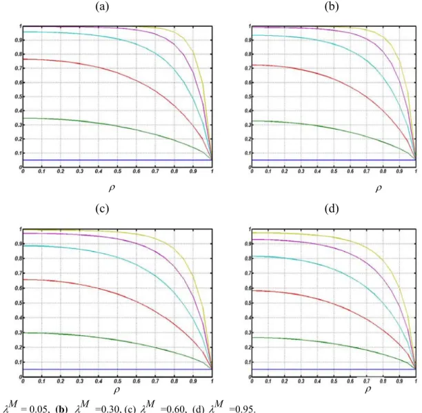
(a) λM = 0.05, (b) λM = 0.30 (c) λM = 0.60, (d) λM = 0.95.

Figure 1 Surface plot of γ for n = 5(1)100 and ρ

∈

[0, 1]

For comparing MSE (

M

~

C

Y_p) with MSE (

M

~

C

_p), we consider the function:

) ~ ( ))

~ ( (

) ~ ( ))

~ ( ( ) ~ (

) ~ ( )

, ,

( ₂

2

p p

Y p Y

p p

Y p M

p

C M Variance C

M bias

C M Variance C

M bias C

M MSE

C M MSE n

MC G

+ + =

=

= λ

γ (14)

ρ ρ

ρ ρ

Equation (14) was written in MATLAB 7.0 software and the three dimensional surface of γ was

obtained. Figure 1 shows the three dimensional surface of γ for MCp = 1.5842 with ρ ∈ [0 , 1] for

different gauge measurement errors (λM ).

According to figure 1, it is obvious that for a known value of measurement capability, the increase

in mean square error of Y

p

MC is more pronounced than that in mean square error of MC_p.

Therefore one can say that for a known value of λM , increasing the correlation coefficient between

process variables and also increasing the sample size will increase the mean square error of MC_p.

Of course, one can see in figure 1 that for a known value of measurement capability and correlation

coefficient, γ increases with the growth of sample size, because the effect of correlation coefficient

and also of measurement errors on process capability estimation is more observable with growing of sample size.

5. CONFIDENCE INTERVAL FOR MCp

Since

M

~

C

_p is a statistical estimator like other statistics, it is subject to the sampling variation,

therefore one needs to compute an interval to provide a range that includes the true MCp with high

probability. Based on the definition, a 100(1−α)% confidence interval for MCp can be established

(Pearn et al.(2007)). 100(1−α)% confidence interval bound can be written as (15):

⎥ ⎥ ⎥ ⎥ ⎦ ⎤ ⎢ ⎢ ⎢ ⎢ ⎣ ⎡ − − − ⎥ ⎥ ⎥ ⎥ ⎦ ⎤ ⎢ ⎢ ⎢ ⎢ ⎣ ⎡ − − − − − − − v Y v p v Y v p v Y p v Y p n F b C M n F b C M or n F C M n F C M ) 1 ( ) 2 ( ) ~ ( , ) 1 ( ) 2 1 ( ) ~ ( ) 1 ( ) 2 ( ) ˆ ( , ) 1 ( ) 2 1 ( ) ˆ ( 1 2 1 2 1 2 1 2 α α α α (15)

Furthermore, a 100(1−α)% lower confidence bound for MCp can be obtained as:

⎥ ⎥ ⎦ ⎤ ⎢ ⎢ ⎣ ⎡ − ⎥ ⎥ ⎦ ⎤ ⎢ ⎢ ⎣ ⎡ − − − v Y v p v Y p n F b C M or n F C M ) 1 ( ) ( ) ~ ( ) 1 ( ) ( ) ˆ

( 2 1 α 2 1 α (16)

However, as a result of the measurement errors, we take Y

p

C

M

~

as an estimator of MCp. Thus the

confidence bounds are:

⎥ ⎥ ⎥ ⎥ ⎦ ⎤ ⎢ ⎢ ⎢ ⎢ ⎣ ⎡ − − − ⎥ ⎥ ⎥ ⎥ ⎦ ⎤ ⎢ ⎢ ⎢ ⎢ ⎣ ⎡ − − − − − − − v Y v Y p v Y v Y p v Y Y p v Y Y p n F b C M n F b C M or n F C M n F C M ) 1 ( ) 2 ( ) ~ ( , ) 1 ( ) 2 1 ( ) ~ ( ) 1 ( ) 2 ( ) ˆ ( , ) 1 ( ) 2 1 ( ) ˆ ( 1 2 1 2 1 2 1 2 α α α α (17) ⎟ ⎟ ⎠ ⎞ ⎢ ⎢ ⎣ ⎡ ∞ − − ⎟ ⎟ ⎠ ⎞ ⎢ ⎢ ⎣ ⎡ ∞ − − − − , ) 1 ( ) 1 ( ) ~ ( , ) 1 ( ) 1 ( ) ˆ

( 2 1 2 Y1 _v

v Y p v Y Y p n F b C M or n F C

M α α (18)

In the discussed example, a 95% confidence interval and lower bound for MCp are given as

It is interesting to find out the confidence coefficient θ (the probability that the confidence interval

contains the actual MCp value) for the confidence bound given in (17). One can calculate this

coefficient using the following definition:

⎟ ⎟ ⎟ ⎟ ⎠ ⎞ ⎜ ⎜ ⎜ ⎜ ⎝ ⎛ + ≤ ≤ + − = ⎟ ⎟ ⎟ ⎟ ⎠ ⎞ ⎜ ⎜ ⎜ ⎜ ⎝ ⎛ − ≤ ≤ − − = − − − − − − − − | | | | | | 2 1 | | | | | | 2 1 1 2 1 2 ) ˆ ˆ ( ) 2 ( ) ˆ ˆ ( ) 2 1 ( ) 1 ( ) 2 ( ) ˆ ( ) 1 ( ) 2 1 ( ) ˆ ( Me Y Me Y Me Y Me Y S S S S p M Y S S S S p M Y v Y Y p p v Y Y p C M F y C M F P n F C M MC n F C M P λ α λ α α α

θ (19)

By substituting y in the above equation we get:

⎟ ⎠ ⎞ ⎜ ⎝ ⎛ ₊ − ⇒ − ⎟ ⎟ ⎠ ⎞ ⎜ ⎜ ⎝ ⎛ − − | | | | | | 2 2 2 2 ) ˆ ˆ ( ) ˆ ( ) 1 ( ˆ ~ ) 1 ( ~ ˆ Me Y Me Y S S S S p M Y p v p v Y p Y p C M C M n C M y n y C M MC λ

If we are interested in evaluating θ for the discussed example, then

θ

=

0

.

5560

, in other words,

the probability that the calculated confidence interval contains the real value of MCp is equal to

0.5560, which is small compared to 0.95. Accordingly, producers will be damaged if they ignore the effect of measurement error on the calculation of confidence interval which will result in rejecting many of their conformed products and making a lot of losses for their process.

In order to improve the confidence interval for the given confidence coefficient (α =1-θ), one can

recalculate the confidence bounds such that it contains the actual value of MCp with the probability

of θ. Hence, if we consider the proposed confidence interval to be L* _{and U}*_{, then with respect to}

the gauge measurement capability, the adjusted 100(1 − α)% confidence interval bound can be

written as (20):

(

)

(

)

) 2 ( ) ˆ ˆ ( ) 1 ( ˆ ) 2 ( , ) 2 1 ( ) ˆ ˆ ( ) 1 ( ˆ ) 2 1 ( 1 2 | | | | | | 2 1 * 1 2 | | | | | | 2 1 * α λ α α λ α − − − − − − − − − − ⎟ ⎠ ⎞ ⎜ ⎝ ⎛ × × = − − − ⎟ ⎠ ⎞ ⎜ ⎝ ⎛ × × − = Y Y p M v S S S S Y p Y Y Y p M v S S S S Y p Y F C M n C M F U F C M n C M F

L Y Me

Me Y Me Y Me Y (20)

For the discussed example, the new confidence interval is given as

L

*

₌

1

.

03073

,

U

*

₌

2

.

4673

_;

therefore, the 0.95 confidence interval for the actual value of MCp is [1.0307 , 2.4673].

Figure 2 shows the changing pattern of θ for different sample sizes, different λMand also different

correlation coefficients at 95% confidence interval.

According to figure 2, one can see that for a known sample size, by growing the amount of

correlation coefficient, the decreasing pattern of confidence coefficient (θ) is affected considerably;

in other words, by increasing the value of correlation coefficient, the effect of measurement

capability on the value of θ will increase and the probability that the 95% calculated confidence

interval contains the true value of MCp will decrease considerably. In addition, one can conclude

that, with growing the value of gauge measurement errors (λM), the effect of correlation

coefficient on reducing the value of confidence coefficient (θ) will increase considerably (figure 2).

Figure 3 shows the curve of the unadjusted lower confidence bound as a function of the correlation

behavior of the adjusted lower confidence bound as a function of the correlation coefficients. In both figures, the upper continuous straight line shows the lower confidence bound for the case of no measurement error, and the striped lines show the lower confidence bounds for different gauge measurement capabilities.

(b) (a)

(d) (c)

(a) λM = 0.05, (b) λM =0.30, (c) r λM =0.60, (d) λM =0.95

Figure 2 Changing procedure of θ with n = 25(25)100 (from bottom to top) and ρin [0, 1]

According to Figure 3, it is obvious that by increasing the measurement capability index, the effect

of correlation coefficient on the lower confidence bound for MC_pwill decrease, such that for large

ρand small λ the change is not considerable, but for large λ the effect of correlation on the lower

confidence bound is noticeable. In other words, the lower confidence bound will be underestimated and it will reduce the precision of estimated process parameters.

The lower bound estimation improves considerably with correcting the lower bound of

Y p

MC (Figure 4), and the effect of this improvement is more observable on the small values of

correlation coefficients.

ρ ρ

ρ ρ

Figure 3 ρ

∈

[0 , 1] for (a) λM = 0.05, (b) λM =0.30, (c) λM =0.60, (d) λM =0.95

Figure 4 ρ

∈

[0 , 1] for (a) λM = 0.05, (b) λM =0.30, (c) λM =0.60, (d) λM =0.95

6. HYPOTHESIS TESTING FOR CAPABILITY INDEX UNDER GAUGE MEASUREMENT ERRORS

In hypothesis testing, we determine whether or not a hypothesized value of a parameter is true based on the sample taken and the parameter estimate derived from it. That is, we are trying to find out where the estimated capability is relative to either true capability, hypothesized capability, or how different the estimated and true capabilities are. To do this, we estimate an index value,

compare it to a lower bound c0, and compute the so-called p-value. The quantity p refers to the

actual risk of incorrectly concluding that the process is capable of a particular test. In general, we want p-value to be no greater than 0.05. To test whether a given process is capable, we may consider the following statistical hypothesis testing:

) (

: 1

) (

: 0

capable is

process c

p MC H

capable not

is process c

p MC H

> ≤

Where c is the standard minimal criteria for MCp. The critical value, c, can be determined as:

α

χ

χ

χ

₋ × ₋ × × ₋ − ≥ = =

= = ≥ ⎟ ⎟ ⎟ ⎟ ⎟ ⎠ ⎞ ⎜ ⎜ ⎜ ⎜ ⎜ ⎝ ⎛ ⎟⎟ ⎠ ⎞ ⎜⎜ ⎝ ⎛ _c p MC c v n v n n n p MC v b P c p MC c p C M P ₀ ) 1 ( 2 ... 2 2 2 1 0

~ ₍₂₁₎

With respect to y=(χ_n2−₁×χ_n2−₂×...×χ_n2−_v), then we have:

2 1 2 0 2 ) ( ) 1 ( 0 2 ) ( ) 1 ( 0 ) 1

( ( ) c

c v b v n c c v b v n y P c v n c v b

P FY

y − = − ≤ → = ≥ − ⎟⎟ → = ⎟ ⎠ ⎞ ⎜ ⎜ ⎜ ⎝ ⎛ ⎟ ⎟ ⎟ ⎠ ⎞ ⎜ ⎜ ⎜ ⎝ ⎛ − _α

α

α

Thus, the critical value can be expressed as:

) 1 ( ) 1 ( 1 0 = − −_−α

Y v v F n c b

c (22)

And the power of the test (the chance of correctly judging a capable process as capable) can be computed as:

{

}

(

)

⎟⎟ ⎟ ⎠ ⎞ ⎜⎜ ⎜ ⎝ ⎛ _{− ×} < = > = − p p v y p p p MC c MC b F y P MC c C M P MC ₂ 2 1 0 ) 1 ( | ˆ ) ( α

π (23)

In the presence of measurement errors, the critical value (denoted by

c

₀Y) α-risk (denoted by

α

Y )

and the power of the test (denoted by

π

Y ) are:

| | | | | | 2 1 0 ) ( 1 ) 1 ( ) 1 ( Me Y Me Y c F n c b c M Y v v Y ∑ − ∑ ∑ − ∑ − + × − − = λ

α (24)

( )

( )

⎟⎟ ⎟ ⎠ ⎞ ⎜ ⎜ ⎜ ⎝ ⎛ + × − < = ∑ − ∑ −∑ ∑ | | | | | | 2 2 0 2 ) ( 1 ) 1 ( Me Y Me Y c c c b n y P M Y v v Y λ

α (25)

(

)

⎟ ⎟ ⎟ ⎠ ⎞ ⎜ ⎜ ⎜ ⎝ ⎛ + × × − < = ∑ − ∑ ∑ − ∑ − p p M p v y p Y _MC MC c MC b F y P MC Me Y Me Y | | | | | | 2 2 2 1 ) ( 1 ) 1 ( ) ( λ α

π (26)

With respect to (25), it can be seen that the right side of this probability equation is multiplied by

1 | | | | | | 2 ) ( _∑∑ ₋−_∑∑ _⎥⎦⎤− ⎢⎣ ⎡ ₊ Me Y Me Y c M

λ . So, we underestimate the true capability of the process when we calculate

than c0 will be less than the probability of that using

M

~

C

p. Thus, the α-risk using

M

~

C

Yp to

estimate MCp is less than the α-risk using

M

~

C

p to estimate MCp (

α

Y ≤α). Also in comparison of

(23) with (26); one can see that equation (26) is multiplied by

[

2 _|| | | _||

]

1

p M Me Y Me Y

)

MC

(

λ

+

_∑∑ ₋−_∑∑ − ; so the

power using

M

~

C

Y_p to estimate MCp is also less than the power using

M

~

C

_p to estimate MCp

(

π

Y ≤

π

).

To improve the method of testing hypothesis for the MCp, one can reconsider the testing procedure

such that in the case of gauge measurement errors, a better estimation of critical region and power of the test is obtained.

If we define

M

~

C

Y_p, using the mentioned definitions in the previous sections then:

v v n n n Y p v Y p v n v

n n Y p Y p v Y p Y p n MC b C M n C M MC b C M MC ) 1 ( ... ~ ) 1 ( ... ~ ~

ˆ 2 2

2 2 1 2 2 2 2 1 − × × × = ⇒ − × × × = − − − − − − χ χ χ χ χ

χ ₍₂₇₎

Therefore, the new α value is given by:

⎟ ⎟ ⎟ ⎟ ⎠ ⎞ ⎜ ⎜ ⎜ ⎜ ⎝ ⎛ = ⎟ ⎠ ⎞ ⎜ ⎝ ⎛ ₊ − < = ⎟ ⎠ ⎞ ⎜ ⎝ ⎛ _{≥ =} = ∑ − ∑ ∑ −

∑ MC c

MC c b n MC y P c C M c C M

P Y_p

p M v v Y p Y p Y p Me Y Me Y ~ ) ( ) 1 ( ~ ~ | | | | | | 2 * 0 2 * 0 * λ α

Based on the above probability phrase, the new critical value is obtained as (28):

[

]

| | | | | | 2 2 / 1 1 2 / * 0 ) ( ) 1 ( ) 1 ( Me Y Me Y c F n c b c M Y v v ∑ − ∑ −∑ ∑ − _{− +} − × × = λ α (28)

Also, to improve the power function of the mentioned testing hypothesis, one can use

M

~

C

Y_p based

on (27):

(

)

⎟ ⎟ ⎟ ⎠ ⎞ ⎜ ⎜ ⎜ ⎝ ⎛ + + × × − < = ⎟ ⎠ ⎞ ⎜ ⎝ ⎛ _{≥ =} = ∑ − ∑ ∑ − ∑ ∑ − ∑ ∑ − ∑ − p p M M p y Y p Y p p MC MC c c MC F y P c C M c C M P MC Me Y Me Y Me Y Me Y | | | | | | 2 | | | | | | 2 2 2 1 * 0 * ) ( ) ( ) 1 ( ~ ~ ) ( λ λ α π (29)

For the discussed example, assume that we want to test the following hypothesis at

(

α

=

0

.

05

)

:

2 : 2 : 1 0 > ≤ p p MC H MC H

Using (24) and (25), the critical value (_cY

0 ), and alpha value (αY) are calculated 3.0179 and 0.001

respectively; so the calculated _αY _{is considerably smaller than the significant level of the test}

((αY =0.001)<(α =0.05) _{), and it will lead to accept the null hypothesis in many cases.}

Accepting the null hypothesis means rejecting the actual capability of the process with respect to consumer view; therefore, it is essential to calculate the critical value by using (28) for testing hypothesis in the presence of measurement errors in order to avoid the false decision.

For the discussed example, the critical value using (28) is c*₀=2.1102. Using this value for testing

hypothesis we get the desired α value (α=0.05). Now if the capability index is increased to

3

MC_p = then the power of the test without considering the measurement error (26) is given as

0677 . 0 )

( _p =

Y _MC

π . If the measurement error is taken into account for evaluating the power of the test

(29), then π*(MCp)=0.5521. Comparing these two values shows that taking into account the gauge

measurement errors will cause a great deal of improvement in testing hypothesis for process capability index.

(b) (a)

(d) (c)

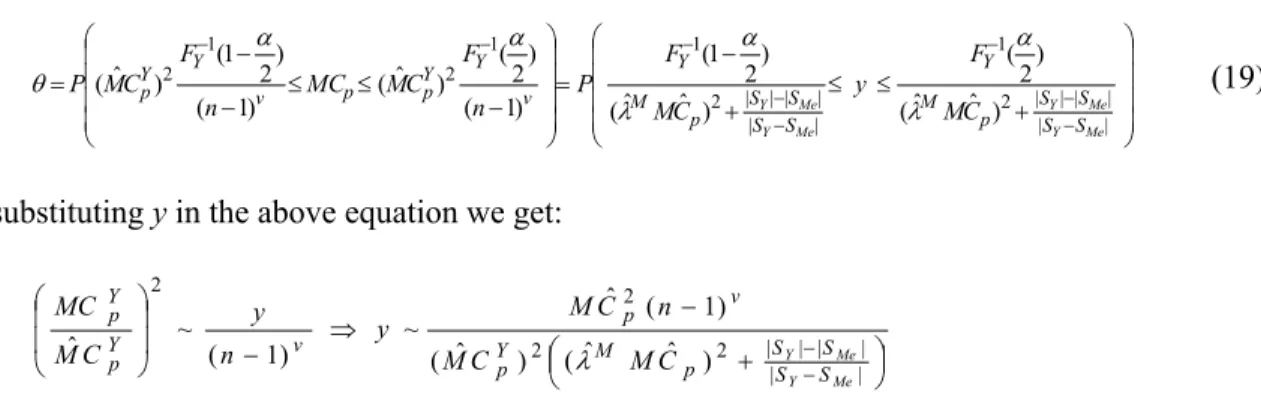
(a)λM= 0.05, (b) λM =0.30, (c) λM =0.60, (d) λM =0.95.

Figure 5 Changing procedure of α (

α

Y_M ) for ρin [0, 1] and n= 5(1)100

ρ ρ

ρ ρ

Figure 5 shows the changing procedure of α ( Y M

α ) according to the changing values of correlation

coefficient, gauge measurement capability and sample size for a type one error probability (α=0.05).

As can be seen, increasing the value of correlation coefficient will reduce the value of

α

Y_M with

respect to themeasurement capability index.

According to figure 5, one can see that with growing the correlation coefficient among process

variables, the

α

Y_M value decreases depending on the measurement capability. So it can be included

that with growing the correlation coefficient and also sample size, the

α

_MY value have a decreasing

behavior depending on measurement capability. On the other hand, whenever the measurement error increases, the effect of correlation coefficient on

α

_MY grows and

α

Y_M decreases considerably.

(b) (a)

(d) (c)

(a) λM= 0.05, (b) λM =0.30, (c) λM =0.60, (d) λM =0.95.

Figure 6 Changing procedure of

π

Y_M(MC_p) versus ρfor MCp =2.00(0.20)3.00 (from bottom to top)

ρ ρ

ρ ρ

Figure 6 shows the changing procedure of unadjusted power of testing ( Y

(

MC

_p

)

M

π

) with different

values of correlation coefficients, gauge measurement capability for different values of deviation

from testing value (c=2). The sample size and α value in this example are n=25 and α=0.05,

respectively.

As it is shown in figure 6, for a given value of measurement capability index, Y ( _p)

M MC

π

decreases

gradually as the correlation coefficient increases. This result shows that the deviation of process capability from the proposed value of c = 2 is not obvious and the testing hypothesis is not confirmed.

(b)

(a)

(d)

(c)

(a)λM= 0.05, (b) λM =0.30, (c) λM =0.60, (d) λM =0.95.

Figure 7 Changing procedure of * ( ) p M MC

π

versus ρfor MCp=2.00(0.20)3.00 (from bottom to top)

ρ ρ

ρ ρ

The effect of correlation coefficient on the adjusted power of the test given by (27) ( * ( ) p M MC

π

)

versus ρfor different measurement capabilities, given sample size (n=25), α=0.05 and c=2 is shown

in figure 7.

According to figure 7, for a given value of Gauge measurement capability, using the adjusted power

of the test ( * ( )

p M MC

π

), the effect of correlation coefficient on the power of the test is negligible for

0 < ρ < 0.7 and the reduced precision is not noticeable.

7. CONCLUSIONS

Most process capability researches in the literatures have been carried out irrespective of gauge measurement errors. Gauge capability has a significant effect on process capability measurement. An inaccurate measurement system can remove the benefits of such endeavors resulting in poor quality. Furthermore, the bulk of the studies associated with analyzing the quality and efficiency of a process are so far limited to discussing one single quality specification, but in real applications, manufactured products often have multiple quality characteristics and multiple characteristics processes are by now so common that our studies on capability indices can't be restricted to the univariate domain. In this paper, we considered the effect of process variables correlation coefficient

on the index MCp for different gauge measurement capabilities. With respect to the results obtained

in this paper, it is specified that gauge measurement capability has an important effect on determining the process capability and this effect grows with increasing the correlation coefficients of process variables. On the other hand, the effect of correlation coefficient on incorrect estimation of

the index MCp increases with growing of the gauge measurement errors.

So, conclusions about capability of the process without considering the gauge measurement capability are not reliable especially in processes with high correlation coefficients. Also we showed

that the α-risk and the power of the test may decrease with a significant magnitude due to gauge

measurement errors, which result in understating capability of the process. Since measurement errors may not be avoided, having proper confidence coefficients and power becomes essential. This necessity will be growing when the correlation coefficient of the process variables increases. Thus, we provided adjusted confidence bounds and critical values for practitioners to use in determining whether their processes meet the capability requirements.

REFERENCES

[1] Boyles R.A. (1996), Exploratory Capability Analysis; Journal of Quality Technology 28; 91–98. [2] Chan L.K., Cheng S.W.; Spiring F.A. (1991), A Multivariate Measure of Process Capability; Journal

of Modeling and Simulation 11; 1–6.

[3] Chang Y.C, Wei Wu, Chien. (2008), Assessing process capability based on the lower confidence bound of Cpk for asymmetric tolerances; European Journal of Operational Research 190; 205-227.

[4] Chen H. (1994), A multivariate process capability index over a rectangular solid tolerance zone; Statistica Sinica 4; 749–758.

[5] Karl D.P., Morisette J.; Taam W. (1994), Some Applications of a Multivariate Capability Index in Geometric Dimensioning and Tolerancing; Quality Engineering 6; 649–665.

[6] Kotz S., Johnson N.L. (2002), Process capability indices – a review, 1992-2000; Journal of Quality Technology 34(1); 1-19.

[7] Montgomery D.C. (1996), Introduction to Statistical Quality Control; 3rd ed, John Wiley & Sons; NewYork, NY.

[8] Montgomery D.C., Runger G.C. (1993), Gauge Capability and Designed Experiments, Part I: Basic Methods; Quality Engineering 6(1); 115-135.

[9] Pearn W.L., Kotz S., Johnson N.L. (1992), Distributional and inferential properties of process capability indices; Journal of Quality Technology 24; 216–231.

[10] Pearn W.L., Liao M.Y. (2005), Measuring process capability based on Cpk with gauge measurement

errors; Microelectronics Reliability 45; 739–751.

[11] Pearn W.L., Kotz S. (2006), Encyclopedia and Handbook of Process Capability Indices. Series on Quality, Reliability and Engineering Statistics, Vol. 12; World Scientific publishing Co, Pte. Ltd. [12] Pearn W.L., Liao M.Y. (2007), Estimating and testing process precision with presence of gauge

measurement errors; Quality and Quantity; Forthcoming.

[13] Pearn W.L., Wang F.K., Chen (2007), Multivariate Capability Indices: Distributional and Inferential Properties; Journal of Applied Statistics 34(8); 941–962.

[14] Shahriari H., Hubele N.F., Lawrence F.P. (1995), A Multivariate Process Capability Vector; Proceedings of the 4th Industrial Engineering Research Conference, Institute of Industrial Engineers; pp 304–309.

[15] Shishebori D., Hamadani A.Z. (2008), The Effect of Gauge Measurement Errors on Multivariate Process Capability, Proceedings of the 3th World Conference on Production and Operations Management (POM), Tokyo, 5-8 August 2008, Chapter 17; pp.2425-2432.

[16] Taam W., Subbaiah P., Liddy J.W. (1993), A Note on Multivariate Process Capability Indices; Journal of Applied Statistics 20(3); 339-351.

[17] Vannman K., Hubele N.F. (2003), Distributional Properties of Estimated Capability Indices Based on Subsamples; Quality and Reliability Engineering International 19; 111–128.

[18] Wang F.K., Du T.C.T. (2000), Using Principal Component Analysis in Process Performance for Multivariate Data; OMEGA, the International Journal of Management Science 28; 185-194.

[19] Wang F.K.; Miskulin J.D, Shahriari H. (2000), Comparison of Three Multivariate Process Capability Indices; Journal of Quality Technology 32(3l); 263-275.

[20] Wang F.K., Chen J. (1998), Capability index using principal component analysis; Quality Engineering 11; 21–27.