Journal of Industrial and Systems Engineering
Vol. 7, No. 1, pp 21 - 42
Autumn 2014
Developing EOQ model with instantaneous deteriorating items for a
vendor-managed inventory (VMI) system
Roya Tat
1, Maryam Esmaeili
1*, Ata Allah Taleizadeh
21
Department of Industrial Engineering, Alzahra University, Tehran, Iran [email protected], [email protected]
2
School of Industrial Engineering, College of Engineering, University of Tehran, Tehran, Iran [email protected]
Abstract
This paper studies the economic-order-quantity model (EOQ) for deteriorating items in two cases (with and without shortages) to evaluate how vendor managed inventory (VMI) affects supply chain. We consider two-level supply chain (single supplier and a single retailer) with one instantaneous deteriorating item. A numerical example and sensitivity analysis are provided to illustrate the effect of related parameters on total cost and optimal order quantity of two systems. The results show that VMI works better and delivers lower cost in all conditions than traditional supply chain (the system before implementation of VMI).
Keywords: Vendor-managed inventory, Supply chain, Economic order quantity
model (EOQ), Deterioration.
1.
Introduction
The effect of deterioration is very important in many inventory systems. Deterioration is explained as decay or damage such that the item cannot be used for its original purpose. Most of the commodities experience decay or deterioration over time. In supply chain management, it is too difficult to protect highly volatile liquids, food stuff, gasoline, liquid medicines, etc., for all business sectors. Owing to this fact, how to control and preserve inventories of deteriorating items becomes a significant problem for decision makers in modern organization.
VMI is an inventory cooperation initiative in supply chain system. Under a VMI system, the vendor decides on the appropriate inventory levels for each product of itself and its retailers, and the proper inventory policies to maintain these levels (Simchi-Livi,Kaminsky and Simchi-Livi, 2008).
*
Corresponding Author
The retailer makes its real-time inventory level accessible for the vendor. In fact in VMI system, the retailer’s role shifts from managing inventory to simply renting retailing space.
We organize the literature review section for both inventory models for deteriorating items and those for VMI systems. Ghare and Schrader (1963) were the pioneers of deteriorating inventory studies who examined the classical no-shortage inventory model with a constant rate of decay. Covert and Philip (1973) extended Ghare and Schrader’s constant deterioration rate to a two-parameter Weibull distribution. Philip (1974) then developed the inventory model with a three-parameter Weibull distribution rate and no shortages. Bahari-Kashani (1989) considered a replenishment schedule for deteriorating items with time-dependent demand. Goswami and Chaudhuri (1992) proposed a deterministic model in which they assumed deterioration is time-proportional and the replenishment rate is directly proportional to the time-dependent demand rate. Kim (1995) presented an inventory replenishment policy for deteriorating items with linearly increasing demand. Bhunia and Maiti (1998) presented an inventory model that assumed deterioration is a linearly increasing function of time. A detailed review of deteriorating inventory literatures is given in Raafat (1991) Goyal and Giri (2001). Lin, Tan and Lee (2000) examined the property of deterioration in EOQ model. They investigated the inventory replenishment policies for the cases with time-varying demand, linearly increasing deterioration rate, partial back-ordering, constant service level and equal replenishment intervals over a fixed planning horizon. Lin and Lin (2004) studied the joint inventory model between supplier and retailer relying on mutual cooperation, for dealing with more general cases they considered the deteriorated rate and partial back-ordering in their assumptions. Ghosh and Chaudhuri (2006) studied an EOQ model over a finite time horizon for a deteriorating item with a quadratic time-dependent demand, considering shortages in inventory. Sana (2010) investigated an EOQ model over an infinite time horizon for deteriorating items while the demand is price-sensitive, allowing partial backordering and time dependent deterioration rate. Khanra, Ghosh and Chuadhuri (2011) developed an EOQ model for a deteriorating item having time dependent demand when delay in payment is permissible. In their model the deterioration rate is assumed to be constant and the time varying demand rate is taken to be a quadratic function of time. Sicilia et al. (2014) studied a deterministic inventory system for items with a constant deterioration rate. In their model demand varies in time and it is assumed that it follows a power pattern. Shortages are allowed and backlogged. The ordering cost, the holding cost, the backlogging cost, the deteriorating cost, and the purchasing cost are considered in the inventory management. An approach is proposed to minimize the total cost per inventory cycle. Guchhait, Maiti and Maiti (2014) developed an inventory model of a deteriorating item with stock and selling price dependent demand under two-level credit period. The model is formulated as retailer’s profit maximization problem for both crisp and fuzzy inventory costs and solved using a modified Genetic Algorithm (MGA).
As a new concept, VMI can be traced back to the classical contribution of Magee(Magee and John, 1958). In recent years; various VMI models were widely studied by researchers. Dong and Xu (2002) presented an analytical model to evaluate the short-term and long term impact of VMI on supply chain profitability by analyzing the inventory systems of the parties involved. Yao, Evers and Dresner (2007) using the same assumptions as Dong with an additional assumption (the order quantity for the supplier is likely to be an integer multiple of the buyer's replenishment quantity) and explored how important supply chain parameters affect the cost savings to be realized from collaborative initiatives such as vendor-managed inventory (VMI). They then determined how the benefits were likely to be distributed between a buyer and a supplier in a supply chain. Ji, Shen and Wei (2008) focused on VMI's role as a strategy of integrated supply chain. This study helps to provide a better understanding of how important supply chain parameters, namely ordering costs and carrying charges, affect the inventory cost savings to be realized from VMI and the distribution of these savings between buyers and suppliers. Darwish and Odah (2010) develop a model for a supply chain with single vendor and multiple retailers under VMI mode of operation. Pasandideh, Akhavan
٢٣
Developing EOQ model with instantaneous deteriorating…
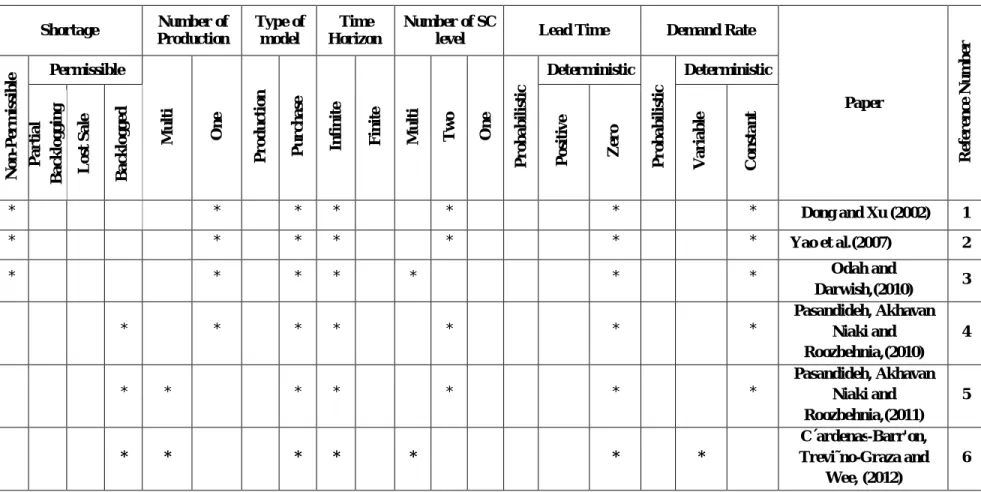
Niaki and Roozbehnia (2010)’s research is the most related one to our paper, they considered the retailer–supplier partnership through a VMI system and developed an analytical model to explore the effect of important supply chain parameters on the cost savings realized from collaborative initiatives. However, their model was an EOQ model with shortage, while our model assumes additional assumption of deterioration rate. In 2011 they developed an economic order quantity (EOQ) model first for a two-level supply chain system consisting of several products, one supplier and one-retailer, in which shortages are backordered, the supplier’s warehouse has limited capacity and there is an upper bound on the number of orders. Since the model of the problem is of a non-linear integer-programming type, a genetic algorithm is then proposed to find the order quantities and the maximum backorder levels such that the total inventory cost of the supply chain is minimized(Pasandideh, Akhavan Niaki and Roozbehnia, 2011). C´ardenas-Barr'on, Trevi˜no-Graza and Wee (2012) presented an alternative heuristic algorithm to solve a multi-product, multi-constraint VMI system based on EOQ with backorders considering two classical backorder costs: linear and fixed. The literature review for deteriorating items and VMI system are summarized in the Tables 1 and 2.
Since the combination of the two respective research streams (inventory models for deteriorating items and those for VMI systems) is scarce, this paper aims to fill the gap and propose vendor-managed inventory (VMI) as one of the new and effective policies for managing inventories in supply chains for deteriorating items.
This paper is organized as follows: Section 2 presents assumption, notation, and the models with the optimal solution regarding shortage and without shortage. Numerical examples are presented in section 3 to analyze the influence of different parameters on the optimal economic order quantity and the total cost before and after implementation of VMI. Finally, conclusions and future research topics are presented in section 4.
Table 1. Deteriorating Items R e fe r e n ce N u m b e r Paper Demand rate Deterioration rate Time horizon
Type of model Shortage Deterministic P r ob ab il is ti c C on stan t V ar iab le F in it e In fi n ite P u r c h a se P r od u cti on Permissible N on -p e r m is si b le C on stan t V ar iab le B ac k log ge d L os t S al e P ar ti al B ac k log gi n g 1
Ghare and Schrader (1963) * * * * * 2
Covert and Philip (1973) * * * * * 3 Philip (1974) * * * * * 4 Bahari-Kashani (1989) * * * * * 5
Goswami and Chaudhuri (1992)
* * * * * 6 Kim (1995) * * * * * 7
Bhunia and Maiti (1998)
* * * * * 8
Lin, Tan and Lee (2000)
* * * * * 9
Lin and Lin (2004)
* * * * * 10
Ghosh and Chaudhuri (2006)
* * * * * 11 Sana (2010) * * * * * 12
Khanra, Ghosh and Chuadhuri (2011)
* * * * 13
Et al. Sicilia (2014)
* * * * * 14
Guchhait, Maiti and Maiti (2014)
* * * * *
٢٥
Developing EOQ model with instantaneous deteriorating…
Table 2. VMI Systems
R e fe r e n ce N u m b e r Paper Demand Rate Lead Time Number of SC
level Time Horizon Type of model Number of Production Shortage Deterministic P r ob ab il is ti c Deterministic P r ob ab il is ti c O n e T w o M u lti F in it e In fi n ite P u r c h as e P r od u cti on O n e M u lti Permissible N on -P er m is si b le C on stan t V ar iab le Z e r o P os iti ve B ac k log ge d L os t S al e P ar ti al B ac k log gi n g 1
Dong and Xu (2002)
* * * * * * * 2
Yao et al.(2007)
* * * * * * * 3 Odah and Darwish,(2010) * * * * * * * 4 Pasandideh, Akhavan Niaki and Roozbehnia,(2010) * * * * * * * 5 Pasandideh, Akhavan Niaki and Roozbehnia,(2011) * * * * * * * 6 C´ardenas-Barr'on, Trevi˜no-Graza and Wee, (2012) * * * * * * *
2.
Model structure
In this research, the problem of a single instantaneous deteriorating product under VMI policy is studied. We construct a two-level supply chain consisting of a single supplier and single retailer and examine the inventory management practices before and after implementation of VMI. We assume that the retailer faces external demand from consumers and investigate the model in two cases including a) shortage is not permitted and b) shortage is permitted and will be fully backordered.
The mathematical models are developed based on the following assumptions:
a) A single- supplier- single-buyer supply chain with one instantaneous deteriorating item is considered.
b) Deliveries of orders are assumed to be instantaneous, that is, the lead time is zero. c) The retailer faces external demand from consumers; Costumer’s demand is deterministic. d) The production rate is infinite.
e) The product will be deteriorated with the fixed rate.
f) There is no repair or replacement of the deteriorated inventory during the period under consideration.
In addition, the following notations are used in model.
The order quantity
The order quantity in VMI policy
The constant rate of instantaneous deterioration
The supplier’s ordering cost per order
The buyer’s ordering cost per order
The deterioration cost per unit
The buyer’s constant demand rate
ℎ
The inventory holding cost held in buyer’s store in a period per unit time
The holding cost rate
(ℎ = < )The maximum level of backordering shortage
The maximum level of backordering in VMI system
The fixed cost of shortage per unit
̂
The cost of shortage per unit per time
The time cycle before VMI
The time cycle after VMI
The percentage of cycle length in which inventory is positive
The buyer’s inventory cost before VMI in case i
The buyer’s inventory cost after VMI in case i
The supplier’s inventory cost before VMI in case i
The supplier’s inventory cost afterVMI in case i
The total cost before VMI
٢٧
Developing EOQ model with instantaneous deteriorating…
2.1.
Case 1. Shortage is not permitted
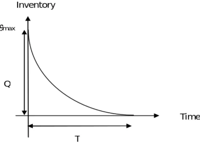
A pictorial description of the inventory policy without shortage is given in Figure 1.
Figure 1. The EOQ model for instantaneous deteriorating items
The inventory level is dropping to zero because of demand and deterioration. So differential equation shown in equation (1) shows the changing the inventory level during0, T.
1
1 dI t
=-θ t I t -D
dt 0≤ ≤ (1)
t t
- βdt T βdt
β(T-t)
0 0
1
t
D
I t =e De dt = e -1
β
(2)
From the Figure 1, since I T =0 &I(0)=Imax=Q we have;
βT
max
D e -1 I(T)=0,I(0)=I =Q ÞQ=
β (3)
The total inventory system cost for the cycle time T is made up of the buyer’s ordering cost, supplier’s ordering cost, product’s carrying cost that held in buyer’s store in a period and deterioration cost. The buyer’s holding cost, is:
Time T
Q max
D DT
2 β
β β T-t
T T
B 1 B
0 0
βT
B B
D e -1
h I (t)dt=h dt
β =h e -1 -h
(4)
Moreover the fixed cost of buyer is ABand the deterioration cost will be;
βT
e -1
C Q-DT =CD -T
β
(5)
2.1.1. Analysis of inventory costs
So prior to implementing VMI, the total cost of the buyer and the total cost of supplier are respectively shown in equation (6) and (7). Then the total cost of the chain is shown in equation (8).
B
βT
T B
01 1
0
e -1 1
KB = A +h I t dt+CD -T
T β
(6)
S 01
A KS =
T (7)
2
βT
B S
01 01
βT
B
D β
e -1
A +A +CD -T
β 1
TC=KB +KS = T
+h e -1-βT
(8)
Using approximation of the Taylor series expansion
2 2
βT β T
e =1+βT+
2 we have;
2
2 2 2
B B
01
1 D β T CDβT
KB = A +h +
T β 2 2
(9)
S 01
A KS =
٢٩
Developing EOQ model with instantaneous deteriorating…
01 01
2 2 2
B B
S 2
B
S B
TC=KB +KS
1 D β T CDβT
= A +A +h +
T β 2 2
A +A h DT CDβT
= + +
T 2 2
(11)
Since
, the total cost function is convex. So the optimal value of T can be
obtained by setting the first derivative of total cost function respect to T equal to zero yielding;
B B
2A T=
h D+CDβ (12)
Therefore;
β T Q = D T 1 +
2
(13)
But under VMI policy, since supplier should pay the buyer costs, then equation (6) to (8) will change to;
11
KB =0 (14)
VMI
VMI
βT
B S B 2 VMI
βT
11 VMI
VMI
D
A +A +h e -1-βT β
1
KS = e -1
T
+CD -T
β
(15)
VMI
VMI
VMI 11 11
βT
B S B 2 VMI
βT VMI
VMI
TC =KB +KS D
A +A +h e -1-βT β
1 =
e -1 T
+CD -T
β
(16)
In this section we use again from approximation of the Taylor series expansion for computational ease.
We can rewrite above formulas as follow:
11
2 2 2
VMI VMI
B B
11 S 2
VMI
β T CDβT
1 D
KS = A +A +h +
T β 2 2
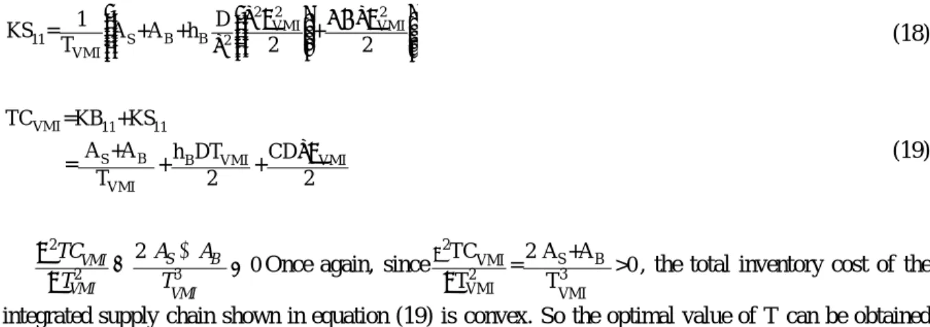
(18)
VMI 11 11
B
S B VMI VMI
VMI TC =KB +KS
A +A h DT CDβT
= + +
T 2 2
(19)
2
2 3
2
0
B S VMI
VMI VMI
A A
TC
T T
Once again, since
2
B S VMI
2 3
VMI VMI
2 A +A TC
= >0
T T
, the total inventory cost of the
integrated supply chain shown in equation (19) is convex. So the optimal value of T can be obtained by setting the first derivative of equation (19) respect to T equal to zero yielding;
S B
VMIB 2 A +A
T =
h D+CDβ (20)
And the order quantity in VMI policy can be determined as below.
VMI
VMI VMI
βT
Q =DT 1+
2
(21)
2.2.
Case 2. Shortage is permitted
In this section, we develop the previous model with an additional assumption that shortage is permitted and will be fully backordered
πˆ0,π=0
. A pictorial description of the inventory policy with shortage is given in Figure 2.Figure 2. The EOQ model for instantaneous deteriorating items with shortage
Time
T
(1-F)T
1(t)
2(t)
Q
b
max
Inventory
٣١
Developing EOQ model with instantaneous deteriorating…
During the time interval0,FTthe inventory level is dropping to zero because of demand and deterioration. So differential equation shown in equation (22) shows the changing the inventory level during0,FT.
1
1 dI (t)
=-θ(t)I (t)-D
dt 0≤ ≤ (22)
Therefore we have;
β(FT-t)
D
e -1
β (23)
Furthermore, at time FT, shortage occurs and the inventory level starts dropping below 0.
2
b 1-F T I t =
2
FT t T (24)
1-F T=bÞb=D 1-F T
D (25)
Therefore we have;
2 2 2
D 1-F T I t =
2 (26)
From the Figure 2, sinceI FT =0 and I(0)=Imax, we have;
max
max
1 0, 0
FT
D e
I FT I I I
(27)
From the Figure 2, since QImaxb we have;
βFT
max
D e -1
Q=I +b= + 1-F TD
β (28)
The total system cost for the cycle time T is made up of the buyer’s ordering cost, supplier’s ordering cost, product’s carrying cost that held in buyer’s store in a period, deterioration cost and cost of shortage. The buyer’s holding cost is:
1
2
β FT-t
FT FT
B B
0 0
βFT
B
D e -1
h I t dt=h dt
β
D
=h e -1-βFT β
(29)
Moreover the fixed cost of buyer is ABand the deterioration cost will be;
βFT max
D e -1-FTβ C I -DFT =C
β (30)
And the Shortage cost is:
2 2 2(t)
ˆ
πD 1-F T ˆ
π×I = 2
(31)
2.2.1. Analysis of inventory costs
So prior to implementing VMI, the total cost of the buyer and the total cost of supplier are respectively shown in equation (32) and (33). Then the total cost of the chain is shown in equation (34).
2 2 FT
B B 1
0
02 βFT
ˆ
πD 1-F T A +h I t dt+
2 1
KB =
T CD e -1-FTβ +
β
(32)
S 02
A KS =
T (33)
02 02
B S B 2
2 2
βFT
βFT
TC=KB +KS D
A +A +h e -1-βFT + β
1 =
CD e -1-FTβ
T πD 1-F Tˆ
+
β 2
(34)
Using approximation of the Taylor series expansion
2 2 2
βFT β F T
e =1+βFT+
٣٣
Developing EOQ model with instantaneous deteriorating…
2 2 2 2 B
B
02 2 2
h DF T CDβF T
A + +
1 2 2
KB =
T πD 1-F Tˆ +
2
(35)
S 02
A KS =
T (36)
2 2 B S B
02 02 2 2 2 2 h DF T
A +A + +
1 2
TC=KB +KS =
T CDβF T πD 1-F Tˆ +
2 2
(37)
The buyer’s inventory cost in Eq.35 is a function of T and F. So, global optimal value of T and F can be obtained by taking the partial derivative of Eq.35 respect to T and F, then setting them equal to zero (in Appendix we prove that T* and F* give a global optimal solution for the EOQ with instantaneous deteriorating items and shortage).
2 2 2
02 B B 2
ˆ πD 1-F KB -A h DF CDβF
= + + +
T T 2 2 2
(38)
02
* B
2 2
B
KB =0 T
2A T F =
ˆ DF h +Cβ +πD 1-F
(39)
02 B KB
ˆ
=h DFT+CDβFT-πD 1-F T F
(40)
* 02
B
KB πˆ
=0 F =
ˆ
F h +Cβ+π
(41)
SubstitutingF*intoT (F) , yields; *
* B B
B
ˆ 2A h +Cβ+π T =
ˆ
h D+CβD π (42)
Considering Eq. 25, amount of shortage before VMI can be calculated as follow:
Considering Eq.35 and Eq.42, the ordering quantity over the cycle before VMI can be determined as:
2 2 max
βF T
Q=I +b=D FT+ + 1-F TD 2 (44)
But under VMI policy, since supplier should pay the buyer costs, then equation (32) to (34) will change to;
12
KB =0 (45)
B S B 2 VMI
VMI 12 VMI 2 2 VMI βFTVMI βFTVMI D
A +A +h e -1-βFT β
CD e -1-FT β 1
KS = +
T β
ˆ
πD 1-F T + 2 (46)
2 2 VMI B S
VMI 12 12 B 2 VMI VMI
VMI
βFTVMI
βFTVMI
ˆ
πD 1-F T
A +A + +
2
1 D
TC =KB +KS = h e -1-βFT
T β
CD e -1-FT β + β (47)
Using approximation of the Taylor series expansion equations (46) and (47) will change to;
2 2
B VMI
B S
12 2 2 2 2
VMI VMI VMI
h DF T
A +A + +
1 2
KS =
T CDβF T πD 1-F Tˆ
+ 2 2 (48)
2 2 VMI S B
VMI 12 12 2 2 2 2 VMI B VMI VMI
ˆ
πD 1-F T A +A +
1 2
TC =KB +KS =
T h DF T CDβF T
+ + 2 2 (49)
Once again, since the total inventory cost in Eq.49 is a function of T and F. So, global optimal value of T and F can be obtained by taking the partial derivative of equation 49 respect to T and F, then setting them equal to zero (as we mentioned in pervious section in Appendix we prove that T* and F* give a global optimal solution for the EOQ with non-instantaneous deteriorating items and shortage).
٣٥
Developing EOQ model with instantaneous deteriorating…
2
B S
VMI B
2
VMI VMI
2 - A +A
TC (h +Cβ)
= + DF
T T 2
ˆ πD 1-F +
2
(50)
VMI VMI
* B S
VMI 2 2
B TC
=0 T
2 A +A
T F =
ˆ DF h +Cβ +πD 1-F
(51)
VMI
B D VMI
C
ˆ
= h F+CβF-π 1-F T F
(52)
* VMI
B
TC πˆ
=0 F =
ˆ
F h +Cβ+π
(53)
Substituting * VMI
F intoTVMI* F , yields;
* B S B
VMI B
2 A +A h +Cβ+πˆ
T =
ˆ
h D+CβD π (54)
Amount of shortage after VMI can be calculated as follow:
VMI VMI VMI
b = 1-F T D (55)
The ordering quantity over the cycle after VMI can be determined as:
max
VMI VMI
2 2
VMI VMI
VMI VMI VMI VMI
Q =I +b =
βF T
D F T + + 1-F T D
2
(56)
3.
Numerical example and sensitivity analysis
In order to illustrate above solution procedure, let us consider an inventory system with the following data:
Table 3. General data
We consider this example for both models. However, in the second model shortage is allowed and completely backlogged
π=80,π=0ˆ
. We solve the example by MATLAB and get following results.D C β
Table 4. The optimal values of decision variables
We now study the effect of changes in the system parametersA ,A ,h ,D,C,S B B βfor both models and
ˆ
just for second model on the optimal order quantity per cycle Q and the total relevant inventory cost
per unite before and after implementation of VMI policy. The sensitivity analysis is performed by changing the parametersA ,A ,h ,D,CS B B by +75%, +50%, +25%, -25%, -50% and -75% , and increasing
β cumulatively at the rate of 0.05 in the interval [0.005,0.5], taking one parameter at a time and
keeping the remaining parameters unchanged. The results are shown in Tables 5 and 6.
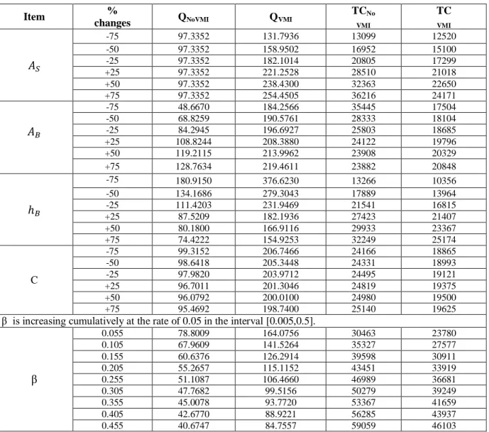
Table 5. Effect of changes in various parameters of the model in case 1
Item %
changes QNoVMI QVMI
TCNo VMI
TC VMI
-75 97.3352 131.7936 13099 12520
-50 97.3352 158.9502 16952 15100
-25 97.3352 182.1014 20805 17299
+25 97.3352 221.2528 28510 21018
+50 97.3352 238.4300 32363 22650
+75 97.3352 254.4505 36216 24171
-75 48.6670 184.2566 35445 17504
-50 68.8259 190.5761 28333 18104
-25 84.2945 196.6927 25803 18685
+25 108.8244 208.3880 24122 19796
+50 119.2115 213.9962 23908 20329
+75 128.7634 219.4611 23882 20848
ℎ
-75 180.9150 376.6230 13266 10356
-50 134.1686 279.3043 17889 13964
-25 111.4203 231.9469 21541 16815
+25 87.5209 182.1936 27423 21407
+50 80.1800 166.9116 29933 23367
+75 74.4222 154.9253 32249 25174
C
-75 99.3152 206.7466 24166 18865
-50 98.6418 205.3448 24331 18993
-25 97.9820 203.9712 24495 19121
+25 96.7011 201.3046 24819 19375
+50 96.0792 200.0100 24980 19500
+75 95.4692 198.7400 25140 19625
β is increasing cumulatively at the rate of 0.05 in the interval [0.005,0.5].
β
0.055 78.8009 164.0756 30463 23780
0.105 67.9609 141.5264 35327 27577
0.155 60.6376 126.2914 39598 30911
0.205 55.2657 115.1152 43451 33919
0.255 51.1087 106.4660 46989 36681
0.305 47.7682 99.5156 50279 39249
0.355 45.0078 93.7720 53367 41659
0.405 42.6770 88.9221 56285 43937
0.455 40.6747 84.7557 59059 46103
case QNoVMI QVMI TCNoVMI TCVMI
1 97.3352 202.6248 24658 19248 2 143.9583 299.6756 16672 13014
٣٧
Developing EOQ model with instantaneous deteriorating…
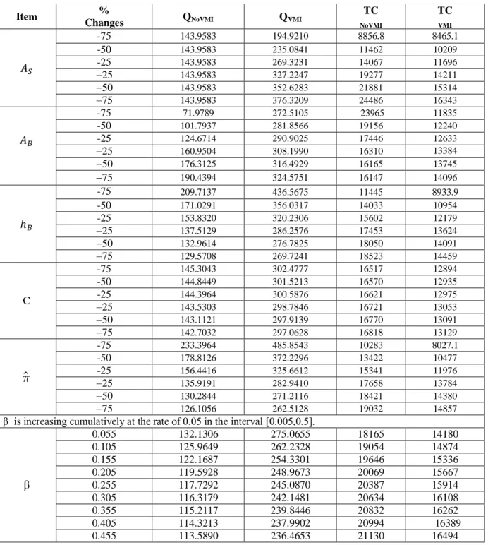
Table 6. Effect of changes in various parameters of the model in case 2
Item %
Changes QNoVMI QVMI
TC NoVMI
TC VMI
-75 143.9583 194.9210 8856.8 8465.1
-50 143.9583 235.0841 11462 10209
-25 143.9583 269.3231 14067 11696
+25 143.9583 327.2247 19277 14211
+50 143.9583 352.6283 21881 15314
+75 143.9583 376.3209 24486 16343
-75 71.9789 272.5105 23965 11835
-50 101.7937 281.8566 19156 12240
-25 124.6714 290.9025 17446 12633
+25 160.9504 308.1990 16310 13384
+50 176.3125 316.4929 16165 13745
+75 190.4394 324.5751 16147 14096
ℎ
-75 209.7137 436.5675 11445 8933.9
-50 171.0291 356.0317 14033 10954
-25 153.8320 320.2306 15602 12179
+25 137.5129 286.2576 17453 13624
+50 132.9614 276.7825 18050 14091
+75 129.5708 269.7241 18523 14459
C
-75 145.3043 302.4777 16517 12894
-50 144.8449 301.5213 16570 12935
-25 144.3964 300.5876 16621 12975
+25 143.5303 298.7846 16721 13053
+50 143.1121 297.9139 16770 13091
+75 142.7032 297.0628 16818 13129
-75 233.3964 485.8543 10283 8027.1
-50 178.8126 372.2296 13422 10477
-25 156.4416 325.6612 15341 11976
+25 135.9191 282.9410 17658 13784
+50 130.2844 271.2116 18421 14380
+75 126.1056 262.5128 19032 14857
β is increasing cumulatively at the rate of 0.05 in the interval [0.005,0.5].
β
0.055 132.1306 275.0655 18165 14180
0.105 125.9649 262.2328 19054 14874
0.155 122.1687 254.3301 19646 15336
0.205 119.5928 248.9673 20069 15667
0.255 117.7292 245.0870 20387 15914
0.305 116.3179 242.1481 20634 16108
0.355 115.2117 239.8446 20832 16262
0.405 114.3213 237.9902 20994 16389
0.455 113.5890 236.4653 21130 16494
Regarding the results obtained from tables 3 and 4, the following analysis are fulfilled:
(a) Increasing supplier’s ordering cost causes no effects on optimal order quantity in both models before implementation of VMI. But, it leads to rise in the optimal order quantity after implementation of VMI. Moreover, increasing supplier’s ordering cost leads to increase of inventory total costs having sharp increase in traditional supply chain. Inventory total costs before and after VMI are close to each other for lower order quantities. But in general, inventory total costs after implementation of
ˆ
VMI are lower than traditional supply chain and this gap will grow by increasing supplier’s ordering cost.
(b) Increasing buyer’s ordering cost in both models leads to increase in optimal order quantity having greater slope in traditional supply chain without VMI. In general, optimal order quantity after VMI is greater than it’s quantity before VMI. Moreover, inventory total cost before VMI has downward trend increasing buyer’s ordering cost, make this trend slighter. However, increasing buyer’s ordering cost leads to increase in inventory total cost after VMI implementation. In general, inventory total costs after implementation of VMI are lower than traditional supply chain.
(c) Increasing buyer’s holding cost in both models eventuate decline in optimal order quantity. But, optimal order quantity is greater after implementing VMI policy. Furthermore, increasing buyer’s holding cost leads to increase in inventory total cost before and after VMI policy. It is obvious that inventory total costs in traditional supply chain are greater than VMI supply chain and this deviation will grow by increasing buyer’s holding cost.
(d) Increasing buyer’s demand rate in both before and after VMI policy, leads to increase in optimal order quantity having greater slope in VMI supply chain. However, optimal order quantity after implementing VMI policy is higher than before it. This distance will grow by increasing demand rate. Moreover, increasing buyer’s demand rate in both before and after VMI policy, leads to increase in inventory total costs. As it observed in those tables, inventory total costs after implementation of VMI are lower than traditional supply chain.
(e) Increasing deterioration cost has a slight effect on optimal order quantity in traditional supply chain and VMI supply chain. As it obvious in the tables, optimal order quantity in VMI supply chain is significantly greater than traditional supply chain. Furthermore, increasing deterioration cost in both before and after VMI policy, eventuates increase in inventory total costs. Inventory total costs after VMI are much less than before VMI implementation.
(f) Increasing deterioration rate leads to decline in optimal order quantity of both models. However, optimal order quantity after VMI policy is greater than the quantity of before it. Furthermore, increasing deterioration rate leads to increase in inventory total cost before and after VMI policy. It is clear that inventory total costs in VMI supply chain are lower than traditional supply chain and this distance will grow with increasing deterioration rate.
(g) According to Table 6, increasing shortage cost eventuate decline in optimal order quantity. But, optimal order quantity after VMI implementation is higher than the before VMI quantity. Furthermore, increasing shortage cost leads to increase in inventory total cost before and after VMI policy. In general, inventory total costs in traditional supply chain are higher than VMI supply chain and this distance will grow with increasing shortage cost.
4.
Conclusions and future research
In this paper, we have considered a two-level supply chain for the EOQ model with single instantaneous deteriorating item to evaluate the performance of the VMI system. The total inventory costs and optimal order quantities have been derived as the performance measures. A numerical example and sensitivity analysis have been provided to illustrate the difference in total cost and optimal order quantity of both systems. It has been demonstrated that the VMI system is more beneficial for the coordination system and delivers lower cost in all conditions including back order. Furthermore, optimal order quantity in all conditions in VMI supply chain is greater than it’s quantity in traditional supply chain.
٣٩
Developing EOQ model with instantaneous deteriorating…
There are a number of directions for future research. For instance, in this study we assumed two-level supply chain with a single deterioration item, while the new model in which one supplier faces two or more buyers could be focused. The model in which the lost sales are considered and also shortage is partial backordering rather than completely backordering could be also investigated.
References
Bahari-Kashani, H. (1989). Replenishment schedule for deteriorating items with
time-proportional demand.
Journal of the Operational Research Society
, 75-81.
Bhunia, A. K., & Maiti, M. (1998). Deterministic inventory model for deteriorating items
with finite rate of replenishment dependent on inventory level.
Computers & operations
research
,
25
(11), 997-1006.
Cárdenas-Barrón, L. E., Treviño-Garza, G., & Wee, H. M. (2012). A simple and better
algorithm to solve the vendor managed inventory control system of product
multi-constraint economic order quantity model.
Expert Systems with Applications
,
39
(3),
3888-3895.
Covert, R. P., & Philip, G. C. (1973). An EOQ model for items with Weibull distribution
deterioration.
AIIE transactions
,
5
(4), 323-326.
Darwish, M. A., & Odah, O. M. (2010). Vendor managed inventory model for single-vendor
multi-retailer supply chains.
European Journal of Operational Research
,
204
(3), 473-484.
Dong, Y., & Xu, K. (2002). A supply chain model of vendor managed inventory.
Transportation Research Part E: Logistics and Transportation Review
,
38
(2), 75-95.
Ghare PM, Schrader GH., (1963). A model for exponentially decaying inventory system, Journal of Industrial Engineering (14). 238-43.
Ghosh, S. K., & Chaudhuri, K. S. (2006). An EOQ model with a quadratic demand,
time-proportional deterioration and shortages in all cycles.
International journal of systems
science
,
37
(10), 663-672.
Goswami, A., & Chaudhuri, K. S. (1992). Variations of order-level inventory models for
deteriorating items.
International Journal of Production Economics
,
27
(2), 111-117.
Goyal, S. K., & Giri, B. C. (2001). Recent trends in modeling of deteriorating inventory.
European Journal of operational research
,
134
(1), 1-16.
Guchhait, P., Maiti, M. K., & Maiti, M. (2014). Inventory policy of a deteriorating item with
variable demand under trade credit period.
Computers & Industrial Engineering
,
76
, 75-88.
Khanra, S., Ghosh, S. K., & Chaudhuri, K. S. (2011). An EOQ model for a deteriorating
item with time dependent quadratic demand under permissible delay in payment.
Applied
Mathematics and Computation
,
218
(1), 1-9.
Kim DH., (1995).A heuristic for replenishment of deteriorating items with linear trend in demand. International Journal of Production Economics (39). 265-70.
Lin, C., & Lin, Y. (2004). A joint EOQ model for supplier and retailer with deteriorating
items.
Asia-Pacific Journal of Operational Research
,
21
(02), 163-178.
Lin, C., Tan, B., & Lee, W. C. (2000). An EOQ model for deteriorating items with
time-varying demand and shortages.
International Journal of Systems Science
,
31
(3), 391-400.
Magee, John F., (1995) .Production planning and inventory control., McGraw Hill, New York.Pasandideh, S. H. R., Niaki, S. T. A., & Nia, A. R. (2011). A genetic algorithm for vendor
managed inventory control system of multi-product multi-constraint economic order quantity
model.
Expert Systems with Applications
,
38
(3), 2708-2716.
Pasandideh, S. H. R., Niaki, S. T. A., & Nia, A. R. (2010). An investigation of
vendor-managed inventory application in supply chain: the EOQ model with shortage.
The
International Journal of Advanced Manufacturing Technology
,
49
(1-4), 329-339.
Pentico, D. W., & Drake, M. J. (2009). The deterministic EOQ with partial backordering: a
new approach.
European Journal of Operational Research
,
194
(1), 102-113.
Philip, G. C. (1974). A generalized EOQ model for items with Weibull distribution
deterioration.
AIIE Transactions
,
6
(2), 159-162.
Raafat, F. (1991). Survey of literature on continuously deteriorating inventory models.
Journal of the Operational Research society
, 27-37.
Sana, S. S. (2010). Optimal selling price and lotsize with time varying deterioration and
partial backlogging.
Applied Mathematics and Computation
,
217
(1), 185-194.
Sicilia, J., González-De-la-Rosa, M., Febles-Acosta, J., & Alcaide-López-de-Pablo, D.
(2014). An inventory model for deteriorating items with shortages and time-varying demand.
International Journal of Production Economics
.
Simchi-Livi, D., Kaminsky, P., Simchi-Livi, E., (2008). Designing and Managing the Supply Chain-Concepts, Strategies and
Case Studies. 3ed, McGraw-Hill, New York.
Yao, Y., Evers, P. T., & Dresner, M. E. (2007). Supply chain integration in vendor-managed
inventory. Decision support systems, 43(2), 663-674.
Wang, C., Ji, S., Shen, J., & Wei, W. (2008, October). Supply chain model in vendor
managed inventory. In Service Operations and Logistics, and Informatics, 2008.
IEEE/SOLI
2008. IEEE International Conference on (Vol. 2, pp. 2110-2113). IEEE.
٤١
Developing EOQ model with instantaneous deteriorating…
Appendix A. proof of the optimality of the solution (41), (42), (53) and (54)
Although the cost function in (35), (49) is not convex, we can prove that (41), (42), (53) and (54) are global optimal using Pentico and Drake (2009)’s method. We can rewrite the cost function as follow:
2
0
1 2 3 3 3
G
TC= +T G +G +G F -2G F+G
T (A1)
Where:
B 0
B S
A=G ;(NoVMI(35):A=A ;
VMI(49):A=A +A ) (A2)
B 1 h D
=G
2 (A3)
2 CDβ
=G
2 (A4)
3 ˆ πD
=G
2 (A5)
Note that all theGis are positive andG >G ,C2 1 β>hB
For ease of notation, we can rewrite (A1) as:
0 G TC=TC(F,T)= +Tr F
T (A6)
Where:
21 2 3 3 3
r F = G +G +G F -2G F+G (A7)
Our objective is to establish the condition under which equation (A6) has a unique interior minimize. Differentiating (A6) with respect to T yields:
F 0 2 G TC
=- +r
T T
(A8)
Which equals zero if and only if T satisfies:
F
F
* G0
T=T =
Note that this is the same result, with appropriate change of notation, gives in (39) and (51). Since the discriminant ofr(F) is negative, r(F) has no roots. Thus, r(F) is either all positive or all negative. Sincer 0 =G >0
3 , r(F) is strictly positive in 0,1. Thus, (A9) gives, for each F, a unique * *
T =T F that minimizes the cost function given by (A6). Substituting the expression forT* F in (A9)
intoTC F,T given by (A6) gives:
*
0
TC F ºTC T F ,F =2 G r F (A10)
Which represent that minimal possible cost for each value of F.
Note thatTC F is continuous, so on the compact interval 0 ,1it has one or more local minima, the
smallest of which will be the global minimum of the cost function. To find these minima, take the first and second derivatives ofTC F with respect to F, yielding:
F F 0
r TC F = G
r
(A11)
3 2
F F F
F
F
2 0
G 2r r - r TC =
2r
(A12)
Note thatTC F, which is, with the change in notation, the same as TC F,T
F
as given in (40) and (52)
is continuous and satisfiesTC 0<0 :
F
1 2 3
3r =2 -G +G +G F-2G (A13)
F
1 2 3
r =2 -G +G +G (A14)
3
0 3 -2G TC 0 = G <0
G
(A15)
The second derivativeTC F given in (A12) factors into:
F
F
3 0 2 1
3 2 2G G G -G
TC =
r
(A16)