Confidence Intervals for the Power of Two-Sided Student’s t-test

(1)

Vol. 8, Nos. 1-2, pp 55-60

Confidence Intervals for the Power of Two-Sided

Student’s t-test

A. Bazargan-Lari1, A. A. Jafari2

1_{Department of Statistics, Islamic Azad University Fars Science & Research} Branch, Shiraz, Iran. (Bazargan-lari@susc.ac.ir)

2_{Department of Statistics, Shiraz University, Shiraz, Iran.}

Abstract. For the power of two-sided hypothesis testing about the mean of a normal population, we derive a 100(1−α)% confidence interval. Then by using a numerical method we will find a shortest confidence interval and consider some special cases.

1 Introduction

SupposeX1, ..., Xnis a random sample of size nfrom a normal

pop-ulation with meanµand variance σ2. The sample mean, ¯X, and the sample variance,S2, are respectively defined as

¯

X= 1

n

n X

i=1

Xi and S2=

1

n

n X

i=1

(Xi−X¯)2.

It is well-known that for testingH◦:µ=µ◦ againstH1 :µ6=µ◦,

with fixed µ0 and significance level α, the relevant test rejects H0

Key words and phrases: Confidence interval, MLE, power of the test, two-sided Student’s t-test.

(2)

whenever

|X¯ −µ◦|> √ S

n−1t1−α/2,n−1

where tp,v is thepth quantiles of the Student’s tdistribution with v

degrees of freedom.

The power function of this test (Lehmann, 1991) is

β(µ, σ) = P(|X¯ −µ◦|> √ S

n−1t1−α/2,n−1) = 1−G_n₋₁_,√

nµ−µ◦_σ (t1−α/2,n−1)

+G_n₋₁_,√

nµ−µ◦_σ (−t1−α/2,n−1). (1)

whereGv,δ(·) is the cumulative distribution function of the noncentral

tdistribution withvdegrees of freedom and noncentrality parameter

δ.

When σ is unknown, we cannot calculate the value of the power functionβ(µ, σ),but it can be estimated by using the invariant prop-erties of Maximum Likelihood Estimators (MLE). Since the MLE of

σ is S,so ˆ

β(µ, σ) = β(µ, S) = 1−G_n₋₁_,√

nµ−µ◦_S (t1−α/2,n−1)

+G_n₋₁_,√

nµ−µ◦_S (−t1−α/2,n−1).

Tarasi´nska (2005) proposed a minimum length method for deter-mining confidence intervals for the power of one-sidedt-test at fixed alternative means. He derived

P(1−G

n−1,∆

√ n b

(t1−α,n−1)< β(∆)<1+G_n₋₁_,∆√n a

(t1−α,n−1)) = 1−γ,

whereβ(∆) =β∗(µ, σ) = 1−G

n−1,∆

√ n σ

(t1−α,n−1) is the power

func-tion of the one-sided Student’s t-test, and ∆ =|µ−µ◦|.

He takes a=

√

nS

√

B and b=

√

nS

√

A. So, for fixed values of n, µ−µ◦

S ,

α, andγ, values ofA and B are found for minimizing

"

β∗(µ,

√

nS

√

B )−β ∗₍_µ,

√

nS

√

A )

#

,

under the condition

Z B

A

f(x)dx= 1−γ,

(3)

where f(x) is the probability density function of chi-squared distri-bution with (n−1) degrees of freedom. With this method the values of Aand B are found numerically.

Now, in this paper we first drive a 100(1−α)% confidence in-terval for the power of two-sided hypothesis testing about the mean of a normal population. Then by the above minimizing method, the shortest confidence intervals are obtained for some special cases.

2 Confidence intervals for the power of the

test

The main results of this section are presented by the following lemma and theorem.

Lemma 2.1. Let us define

h(δ) =Gv,δ(t)−Gv,δ(−t), in which t >0,is constant. Then

i) For all δ >0, the function h(δ) is a decreasing function .

ii) For all δ <0, the function h(δ) is an increasing function.

iii) h(δ) is an even function, that is h(−δ) = h(δ).

Proof.

i) Following Owen (1968), we have

Gv,δ(t) =

√

2π

Γ(v/2)2(v−2)/2 Z ∞

0

uv−1Φ(√tu

v −δ)φ(u)du,

where Φ(·) and φ(·) are the cdf and pdf of the standard normal dis-tribution, respectively. LetC =

√

2π

Γ(v/2)2(v−2)/2, then h(δ) =C

Z ∞

0

uv−1φ(u)

Φ(√tu

v−δ)−Φ(

−tu

√

v −δ)

du. (2)

In (2), letk(δ) = Φ(x−δ)−Φ(−x−δ) andx= √tu

v.We have

k0(δ) =φ(x+δ)−φ(x−δ) = √1

2πe

−1 2 (x

2₊_δ2₎

(e−xδ−exδ).

(4)

Since δ >0 andx >0, sok0(δ)<0. Thereforek(δ) and alsoh(δ) are decreasing functions of δ.

ii) The proof of this part is similar to the proof of part (i). iii) By direct use of (2), we get

h(−δ) = C

Z ∞

0

uv−1φ(u)

Φ(√tu

v +δ)−Φ(

−tu

√

v +δ)

du

= C

Z ∞

0

uv−1φ(u)

Φ(√tu

v +δ)−

1−Φ(√tu

v −δ)

du

= C

Z ∞

0

uv−1φ(u)

Φ(√tu

v −δ)−Φ(

−tu

√

v −δ)

du

= h(δ).

Since the value of β(µ, σ) for µ > µ◦ is equal to the value of

β(µ, σ) for µ < µ◦, we will find the confidence interval for β(µ, σ),

when µ > µ◦.

Theorem 2.1. Let (a,b) be any 100(1−γ)% confidence interval for σ, then

Pn1−G_n₋₁_,√

nµ−µ◦_b (t1−α/2,n−1) +Gn−1,√nµ−µ◦_b (−t1−α/2,n−1)

< β(µ, σ)<

1−G_n₋₁_,√

nµ−µ◦_a (t1−α/2,n−1) +Gn−1,√nµ−µ◦_a (−t1−α/2,n−1) o

= 1−γ. (3)

Proof. Since µ > µ◦,by part (i) of Lemma 2.1, we have 1−γ = P(a < σ < b)

⇐⇒ 1−γ = P(µ−µ◦

b

√

n < µ−µ◦ σ

√

n < µ−µ◦ a

√

n)

⇐⇒ 1−γ = P(β(µ, b)< β(µ, σ)< β(µ, a)).

Therefore, by using (1), we obtain (3).

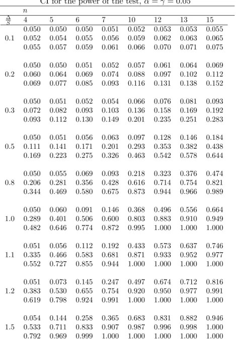
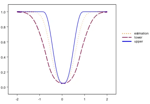
Using R software version 2.7.0., the minimum length method was carried out numerically, with steps equal to .001. Table 1 presents the estimates of the power of the test (the middle value in the cell), and the bounds for 95% confidence intervals of the power with α= 0.05. The curve of the bounds and of the estimate as functions of µ−µ◦

S for

n= 10 are given in Fig 1.

We note again that all the entries in Table 1 are also good for the case µ < µ◦.

(5)

Table 1. Values of lower bound of CI, estimate and upper bound CI for the power of the test, α=γ = 0.05

n

∆

S 4 5 6 7 10 12 13 15

0.050 0.050 0.050 0.051 0.052 0.053 0.053 0.055 0.1 0.052 0.054 0.055 0.056 0.059 0.062 0.063 0.065 0.055 0.057 0.059 0.061 0.066 0.070 0.071 0.075 0.050 0.050 0.051 0.052 0.057 0.061 0.064 0.069 0.2 0.060 0.064 0.069 0.074 0.088 0.097 0.102 0.112 0.069 0.077 0.085 0.093 0.116 0.131 0.138 0.152 0.050 0.051 0.052 0.054 0.066 0.076 0.081 0.093 0.3 0.072 0.082 0.093 0.103 0.136 0.158 0.169 0.192 0.093 0.112 0.130 0.149 0.201 0.235 0.251 0.283 0.050 0.051 0.056 0.063 0.097 0.128 0.146 0.184 0.5 0.111 0.141 0.171 0.201 0.293 0.353 0.382 0.438 0.169 0.223 0.275 0.326 0.463 0.542 0.578 0.644 0.050 0.055 0.069 0.093 0.218 0.323 0.376 0.474 0.8 0.206 0.281 0.356 0.428 0.616 0.714 0.754 0.821 0.344 0.469 0.580 0.675 0.873 0.944 0.966 0.989 0.050 0.060 0.091 0.146 0.368 0.496 0.556 0.664 1.0 0.289 0.401 0.506 0.600 0.803 0.883 0.910 0.949 0.482 0.646 0.774 0.872 0.995 1.000 1.000 1.000 0.051 0.056 0.112 0.192 0.433 0.573 0.637 0.746 1.1 0.335 0.466 0.583 0.681 0.871 0.933 0.952 0.977 0.552 0.727 0.855 0.944 1.000 1.000 1.000 1.000 0.051 0.073 0.145 0.247 0.497 0.674 0.712 0.816 1.2 0.383 0.530 0.655 0.754 0.920 0.950 0.977 0.991 0.619 0.798 0.924 0.991 1.000 1.000 1.000 1.000 0.054 0.144 0.258 0.365 0.683 0.831 0.882 0.946 1.5 0.533 0.711 0.833 0.907 0.987 0.996 0.998 1.000 0.792 0.969 0.999 1.000 1.000 1.000 1.000 1.000

(6)

Fig. 1. CI curves (95%) for the test power and the estimate of the power (the middle one) as the functions of µ−µ◦

S ,n= 10,α= 0.05

Acknowledgements

The authors are grateful to the editor and two referees for their help-ful comments and suggestions which led to the improvement in the presentation of the paper. The first author also thanks the Research Council of Islamic Azad University Fars Science & Research Branch, for their support.

References

Lehmann, E. L. (1991), Testing Statistical Hypothesis. New York: Wiley.

Owen, D. B. (1968), A survey of properties and applications of the noncentral t-distribution. Technometrics, 10, 445-478.

Tarasi´nska, J. (2005), Confidence interval for the power of student’s t-test. Statistics & Probability Letter,73, 125-130.

-2 -1 0 1 2

0.0 0.2 0.4 0.6 0.8 1.0

estmation lower upper