Modelling Dispersion Characteristics of Circular
Optical Waveguide with Helical Winding–
Comparison for Different Pitch Angles
A.K. Gautam* and V. MishraDepartment of Electronics Engineering, Sardar Vallabhbhai National Institute of Technology, Surat, India
*
Corresponding Author: [email protected]
Abstract— In this Article dispersion characteristic of conventional optical waveguide with helical winding at core – cladding interface has been obtained. The model dispersion characteristics of optical waveguide with helical winding at core-cladding interface have been obtained for five different pitch angles. This paper includes dispersion characteristics of optical waveguide with helical winding, and compression of dispersion characteristics of optical waveguide with helical winding at core-cladding interface for five different pitch angles. Boundary conditions have been used to obtain the dispersion characteristics and these conditions have been utilized to get the model Eigen values equation. From these Eigen value equations dispersion curve are obtained and plotted for modified optical waveguide for particular values of the pitch angle of the winding and the result has been compared.
KEYWORDS: Optical fiber communication,
fiber dispersion, helical winding, helix pitch angle, modal cutoff.
I.
I
NTRODUCTIONOptical fibers with helical winding are known as complex optical waveguides. The use of helical winding in optical fibers makes the analysis much accurate [1]. Singh [13] have proposed an analytical study of dispersion characteristics of helically cladded step –
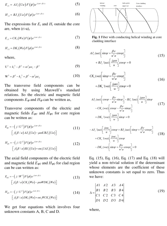
the core–cladding boundary surfaces. We assume that the waveguide have real constant refractive index of core and cladding is n1 and n2 respectively (n1>n2).
II.
T
HEORY ANDC
ALCULATIONS The optical waveguide is the fundamental element that interconnects the various devices of an optical integrated circuit, just as a metallic strip does in an electrical integrated circuit. The mode theory [10] is used to describe the properties of light that ray theory is unable to explain. A set of guided electromagnetic waves is called the modes [13, 16] of the fiber. For a given mode, a change in wavelength can prevent the mode from propagating along the fiber. The mode is no longer bound to the fiber. The mode is said to be cut off [13]. The wavelength at which a mode ceases to be bound is called the cutoff wavelength [11] for that mode. we consider the following boundary conditions [8].1 1 0
z
E sinψ +E cosφ ψ = (1)
2 2 0
z
E sinψ +E cosφ ψ = (2)
(
Ez1−Ez2)
cosψ −(
Eφ1−Eφ2)
sinψ =0 (3)(
Hz1−Hz2)
sinψ +(
Hφ1−Hφ2)
cosψ =0 (4)( ) ( )
( ) 1 1j t z
z
E =AJ Ua F φ e ω β− (5)
( ) ( ) ( )
1 1
j t z z
H =BJ Ua F φ e ω β− (6)
The expressions for Ez and Hz outside the core are, when (r>a),
( ) ( ) ( )
2 1
j t z z
E =CK Wa F φ e ω β− (7)
( ) ( ) ( )
2 1
j t z z
H =DK Wa F φ e ω β− (8)
where,
2 2 2 2 2
1 1
U =k –β =ω με −β (9)
2 2 2 2 2
2 2
W =β −k =β −ω με (10)
The transverse field components can be obtained by using Maxwell’s standard relations. So the electric and magnetic field components Eϕand Hϕ can be written as, Transverse components of the electric and magnetic fields Eϕ1 and Hϕ1 for core region can be written as:
(
)
( )( ) ( ) ( )
2 ( )
1
'
1 1
/ /
j t z
E j U F e
j a AJ Ua UBJ Ua
ω β φ φ β μω − = − ⎡ − ⎤ ⎣ ⎦ (11)
(
)
( ) ( ) ( ) ( )2 ( )
1
'
1 1 1
/ /
j t z
H j U F e
j a BJ Ua UAJ Ua
ω β φ φ β ωε − = − ⎡ + ⎤ ⎣ ⎦ (12)
The axial field components of the electric field and magnetic field Eϕ2 and Hϕ2 for clad region can be can written as:
(
)
( )( ) ( ) ( )
2 ( )
2
'
1 1
/
/
j t z
E j W F e
j a CK Wa WDK Wa
ω β φ φ β μω − = − ⎡ − ⎤ ⎣ ⎦ (13)
(
)
( ) ( ) ( ) ( )2 ( )
2
'
1 2 1
/ /
j t z
H j U F e
j a DK Wa WCK Wa
ω β φ φ β ωε − = − ⎡ + ⎤ ⎣ ⎦ (14)
We get four equations which involves four unknown constants A, B, C and D.
Fig. 1 Fiber with conducting helical winding at core cladding interface
2
( ) sin cos
'( ) cos 0
AJ ua u a j BJ ua u ν ν βν ψ ψ μω ψ ⎡ + ⎤ ⎢ ⎥ ⎣ ⎦ ⎡ ⎤ + ⎢ ⎥ = ⎣ ⎦ (15) 2
( ) sin cos '( ) cos 0
CK wa w a j DK wa w ν ν βν ψ ψ μω ψ ⎡ + ⎤ ⎢ ⎥ ⎣ ⎦ ⎡ ⎤ + ⎢ ⎥ = ⎣ ⎦ (16) 2 2
( ) cos sin '( ) sin
( ) cos sin
'( ) sin 0 j
AJ ua BJ ua
u a u
CK wa w a j DK wa w ν ν ν ν βν μω
ψ ψ ψ
βν ψ ψ μω ψ ⎡ − ⎤− ⎡ ⎤ ⎢ ⎥ ⎢ ⎥ ⎣ ⎦ ⎣ ⎦ ⎡ ⎤ − ⎢ − ⎥ ⎣ ⎦ ⎡ ⎤ + ⎢ ⎥ = ⎣ ⎦ (17) 1 2 2 2
'( ) cos ( ) sin cos
'( ) cos
( ) sin cos 0 j
AJ ua BJ ua
u u a
j CK wa w DK wa w a ν ν ν ν
ωε ψ ψ βν ψ
ωε ψ βν ψ ψ ⎡ ⎤ ⎡ ⎤ − ⎢ ⎥ + ⎢ + ⎥ ⎣ ⎦ ⎣ ⎦ ⎡ ⎤ + ⎢ ⎥ ⎣ ⎦ ⎡ ⎤ − ⎢ + ⎥= ⎣ ⎦ (18)
Eq. (15), Eq. (16), Eq. (17) and Eq. (18) will yield a non–trivial solution if the determinant whose elements are the coefficient of these unknown constants is set equal to zero. Thus we have:
1 2 3 4
1 2 3 4
1 2 3 4
1 2 3 4
Δ =
A A A A
B B B B
C C C C
D D D D
(19)
where,
2
1 ( ) sin cos
2 '( ) cos
⎡ ⎤ = ⎢ + ⎥ ⎣ ⎦ ⎡ ⎤ = ⎢ ⎥ ⎣ ⎦
A J ua
u a j
A J ua
u ν
ν
βν
ψ ψ
μω ψ (20)
3= 4= 1= 2=0
A A B B
2
3 ( ) sin cos
4 '( ) cos
⎡ ⎤ = ⎢ + ⎥ ⎣ ⎦ ⎡ ⎤ = ⎢ ⎥ ⎣ ⎦
B K wa
w a j
B K wa
w ν
ν
βν
ψ ψ
μω ψ (21)
2
2
1 ( ) cos sin
2 '( ) sin
3 ( ) cos sin
4 '( ) sin
C J ua
u a j
C J ua
u
C K wa
w a j
C K wa
w ν ν ν ν βν ψ ψ μω ψ βν ψ ψ μω ψ ⎡ ⎤ = ⎢ − ⎥ ⎣ ⎦ ⎡ ⎤ = − ⎢ ⎥ ⎣ ⎦ ⎡ ⎤ = − ⎢ − ⎥ ⎣ ⎦ ⎡ ⎤ = ⎢ ⎥ ⎣ ⎦ (22) 1 2 2 2
1 '( ) cos
2 ( ) sin cos
3 '( ) cos
4 ( ) sin cos
j
D J ua
u
D J ua
u a j
D K wa
w
D K wa
w a ν ν ν ν ωε ψ βν ψ ψ ωε ψ βν ψ ψ ⎡ ⎤ = − ⎢ ⎥ ⎣ ⎦ ⎡ ⎤ = ⎢ + ⎥ ⎣ ⎦ ⎡ ⎤ = ⎢ ⎥ ⎣ ⎦ ⎡ ⎤ = − ⎢ + ⎥ ⎣ ⎦ (23)
After simplifying the determinant, we get a simplified equation for lowest order modes.
1
2
2 2 '
2
1 1
' 2
1 1
2 2 '
2
1 1
' 2
1 1
( ) ( )
sin cos cos
( ) ( )
( ) ( )
sin cos cos 0
( ) ( )
k
J Ua J Ua
U
J Ua U a U J Ua
k
K Wa K Wa
W
K Wa W a W K Wa
β
ψ ψ ψ
β
ψ ψ ψ
⎛ + ⎞ − ⎜ ⎟ ⎝ ⎠ ⎛ ⎞ − ⎜ + ⎟ + = ⎝ ⎠ (24)
III.
R
ESULTSIt is now possible to interpret the characteristic equation (Eq. 24) in numerical terms. This will give us an insight into model properties of our waveguide. For this we can use following relations, 1 2 2 1 ' 2 1 2 ' 2 1 1 2 1 ' 2 1 2 ' 2 1 1 ( ) sin cos ( ) ( ) cos ( ) ( ) sin cos ( ) ( ) cos 0 ( ) J Ua U
J Ua U a
k J Ua U J Ua K Wa W
K Wa W a
k K Wa W K Wa
β ψ ψ ψ β ψ ψ ψ ⎛ + ⎞ ⎜ ⎟ ⎝ ⎠ − ⎛ ⎞ − ⎜ + ⎟ ⎝ ⎠ + = (25)
2 2 2
2 2 2 1 2
( / )k n
aw b
V n n
β
⎛ − ⎞
⎛ ⎞
=⎜ ⎟ = ⎜ ⎟
−
⎝ ⎠ ⎝ ⎠ (26)
2
2 2 2 2 2 2
1 2
2
( ) a ( )
V u w a π n n
λ
⎛ ⎞
= + =⎜ ⎟ −
⎝ ⎠ (27)
where b and V are known as normalization propagation constant and normalized frequency parameter respectively. We make some simple calculations based. We choose
n1=1.50, n2=1.46 and λ=1.55µm.
A. Dispersion Curve
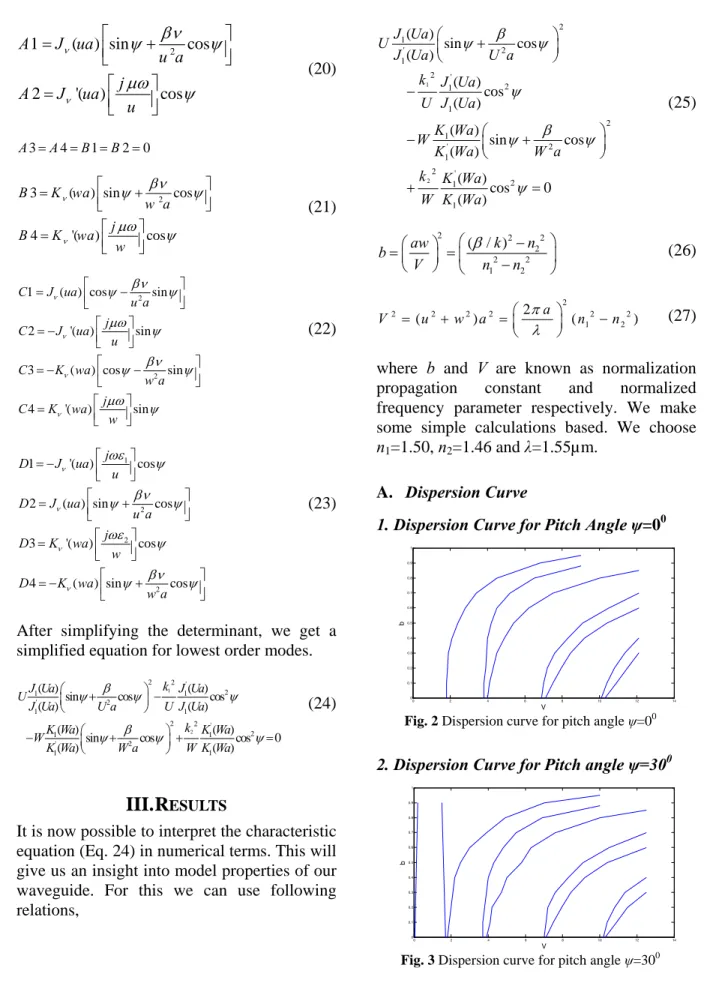
1. Dispersion Curve for Pitch Angleψ=00
0 2 4 6 8 10 12 14
0 0.1 0.2 0.3 0.4 0.5 0.6 0.7 0.8 0.9 1 V b
Fig. 2 Dispersion curve for pitch angle ψ=00
2. Dispersion Curve for Pitch angle ψ=300
0.1 0.2 0.3 0.4 0.5 0.6 0.7 0.8 0.9 1 b
3. Dispersion Curve for Pitch Angle ψ=450
0 2 4 6 8 10 12 14
0 0.1 0.2 0.3 0.4 0.5 0.6 0.7 0.8 0.9 1
V
b
Fig. 4 Dispersion curve for pitch angle ψ=450
4. Dispersion Curve for Pitch Angle ψ=600
0 2 4 6 8 10 12 14
0 0.1 0.2 0.3 0.4 0.5 0.6 0.7 0.8 0.9 1
V
b
Fig. 5 Dispersion curve for pitch angle ψ=600
5. Dispersion Curve for Pitch Angle ψ=900
0 2 4 6 8 10 12 14
0 0.1 0.2 0.3 0.4 0.5 0.6 0.7 0.8 0.9 1
V
b
Fig. 6 Dispersion curve for pitch angle ψ=900 We observed that, they all have standard expected shape. This effect is undesirable for the possible use of. This means that one effect of conducting helical winding is to these waveguide for long distance communication in pairs that is cutoff values for two adjacent modes converge.
We found that some curves have band gaps of discontinuities between some value of V. These represent the band gaps or forbidden bands of the structure. These are induced by
B. Dependence of Cutoff Values on Pitch
Angle
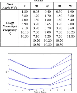
From Table I, we note particularly that the dependence of the cutoff V–value (Vc) on ψ is such that as ψ is increased, there is a drastic fall in Vc at ψ=300, and then a small increase as ψ goes from 300 to 600; then there is a quick rise as ψ changes from 600 to 900 (Fig. 7). Thus the two most sensitive regions in respect of the influence of helical pitch angle ψ on the cutoff values and the model properties of waveguides are ranges from ψ=00 to ψ=300 and ψ=600 to ψ=900 and these ranges of pitch angle expected to have potential applications with ψ as a means for controlling the model properties split the modes and remove a degeneracy which is hidden in conventional waveguide without windings.
TABLEICUTOFF VCVALUES FOR SOME LOWER ORDER
MODES
Pitch
Angle Ψ(0) 0 30 45 60 90
1.80 0.05 0.40 0.30 1.90 3.80 1.70 1.70 1.50 3.80 4.00 1.80 1.80 1.80 5.40 6.90 3.70 3.65 3.70 7.00 7.10 3.90 3.70 3.90 8.60 10.10 7.00 7.00 7.00 10.20 10.30 7.10 7.20 7.20 11.80 - 10.20 10.20 10.20 -
Cutoff Normalized
Frequency Vc
- 10.30 10.30 10.30 -
0 10 20 30 40 50 60 70 80 90
0 2 4 6 8 10 12
Angle in Degree
Vc
Fig. 7 Dependence of cutoff values Vc on the pitch angle ψ
IV.
C
ONCLUSIONWe observed that, they all have standard expected shape, but except for lower order modes they comes in pairs, that is cutoff values for two adjacent mode converge. This
means that one effect of conducting helical winding is to split the modes and remove a degeneracy which is hidden in conventional waveguide without windings.
From the above discussions we can conclude that the modal cutoff for helical pitch angle
ψ=300, 450 and 600 are higher than the modal cutoff for helical pitch angle ψ=00 and 900. This means, for some specific range of cutoff values Vc, one can have greater number of modes for helical pitch angle ψ=300, 450 and 600 than for helical pitch angle ψ=00 and 900. So the helical pitch angle ψ=300, 450 and 600 are better than helical pitch angle ψ=00 and 900.
R
EFERENCES[1] D. Kumar, and O.N. Singh II, “Modal
characteristics equation and dispersion curves for an elliptical step-index fiber with a conducting helical winding on the core-cladding boundary - An analytical study,” IEEE, J. Lightwave Technol. Vol. 20, pp. 1416–1424, 2002.
[2] D.A. Watkins, Topics in Electromagnetic
Theory, John Wiley and Sons Inc., NY, 1958.
[3] V.N. Mishra, V. Singh, B. Prasad, and S.P. Ojha, “Optical Dispersion curves of two metal-clad light guides having double convex lens core cross sections,” Microwave Opt. Technol. Lett. Vol. 24, pp. 229-232, 2000.
[4] V.N. Mishra, V. Singh, B. Prasad, and S.P. Ojha, “An Analytical investigation of dispersion characteristic of a light guide with an annular core cross section bounded by two cardioids,” Microwave Opt. Technol. Lett., Vol. 24, pp. 229-232, 2000 and Microwave Opt. Technol. Lett., Vol. 16, pp. 213-221, 1999.
[5] V. Singh, S.P. Ojha, B. Prasad, and L.K.
Singh, “Optical and microwave Dispersion curves of an optical waveguide with a guiding region having a core cross section with a lunar shape,” Optik, Vol. 110, pp. 267-270, 1999.
[6] V. Singh, S.P. Ojha, and L.K. Singh, “Model
Microwave Opt. Technol. Lett. Vol. 21, pp. 121-124, 1999.
[7] V. Singh, S.P. Ojha, and B. Prasad, “Weak guidance modal dispersion characteristics of an optical waveguide having core with sinusoidally varying gear shaped cross section,” Microwave Opt. Technol. Lett. Vol. 22, pp. 129-133, 1999.
[8] D. Gloge, “Dispersion in weakly guiding
fibers,” Appl. Opt. Vol. 10, pp. 2442-2445, 1971.
[9] P.K. Choudhury, D. Kumar, Z. Yusoff, and
F.A. Rahman, “An analytical investigation of four-layer dielectric optical fibers with au nano-coating - A comparison with three-layer optical fibers,” PIER Vol. 90, pp. 269-286, 2009.
[10]G. Keiser, Optical Fiber Communications, Chap. 2, 3rd ed. McGraw-Hill, Singapore, 2000.
[11]J. Ming-Liu, Photonic Devices, Cambridge University Press, UK, 2005.
[12]D. Kumar and O.N. Singh II, “Towards the dispersion relations for dielectric optical fibers with helical windings under slow and fast wave considerations – a comparative analysis,” PIER, Vol. 80, pp. 409-420, 2008.
[13]D. Kumar and O.N. Singh II, “An analytical study of the modal characteristics of annular step-index fiber of elliptical cross–section with two conducting helical windings on the two boundary surfaces between the guiding and non–guiding regions,” Optik, Vol. 113, pp. 193-196, 2002.
[14]U.N. Singh, O.N. Singh II, P. Khastgir, and K. K. Dey “Dispersion characteristics of helically cladded step – index optical fiber analytical study,” J. Opt. Soc. Am. B, Vol. 12 , pp. 1273-1278, 1995.
[15]M.P.S. Rao, V. Singh, B. Presad, and S.P. Ojha “Model characteristic and dispersion curves of hypocycloidal optical waveguide,” Optik, Vol. 110, pp. 81-85, 1999.
[16]A. Ghatak and K. Thyagarajan, Optical
Electronics, Cambridge University Press, India, 2008.
boundary – An analytical treatment,” Optik Vol. 112, pp. 561-566, 2001.
[18]G. P. Agrawal, Fiber Optic Communication
Systems, 3rd ed. John Wiley and Sons, Inc., New York, 2002.
Ajay Kumar Gautam was born in Bareilly (UP), India, in 1983. He pursued his Bachelor of Technology from Uttar Pradesh Technical University (U. P.) India in 2007, and completed Master of Technology from Sardar Vallabhbhai National Institute of Technology, Surat (Gujarat), India in 2010. He is working as Assist. Professor at Dev Bhoomi Group of Institutions, Dehradun, India. He published more than 5 papers in various National and International Journals.
V. Mishra was born in UP, India, in 1973. He received Bachelor and Master of Sciences from Purvanchal University U. P. India, and completed Doctor of Philosophy from Institute of Technology B. H. U. India in 2001. He worked as Lecturer in Multimedia University and then Assistant Professor in UTAR, Malaysia for nine years and now working as Associate professor in SVNIT, Surat, Gujarat, India. Dr. Mishra is member and chairperson for many Research Centers of Excellence in MMU, Malaysia. He is a senior Member of IEEE, Fellow of IETE, and published more than 60 papers in various National and International Journals. He has completed two external projects Funded by E-Science, Malaysian Government, and working on three projects from DST and DRDO India.