The Texture Animator
Damjan Strnad and Nikola Guid
Faculty of Electrical Engineering and Computer Science, University of Maribor, Slovenia
This paper discusses three distinct techniques for anima-tion of procedural textures and describes the assisting software tool. Animation is attained by moving the rendered point before texture evaluation, changing the definition of texture space or changing the texture colour mapping. Examples are given for textures that base on noise and turbulence functions in order to simulate natural phenomena. Some phases of texture animation process can be automated by using the code generator supported by a library of animation effects. Aspects of practical implementation are discussed and Renderman compliant code is presented.
Keywords: texture animation, procedural texture, code generator, Renderman specification
1. Introduction
Texturing is one of fundamental procedures in modern computer graphics. It significantly increases image realism and is essential for achieving the so-called photo-realism in arti-ficially constructed and rendered scenes. Tex-tures may be derived by scanning a photo or they can be procedurally defined. Procedural textures are today’s topic. They can be defined over arbitrary number of dimensions, although 3D solid textures get most practical use today. Procedural texture value is determined by pro-gram code and interpretation of that value de-pends on the renderer. The most common use of textures is surface colour representation that will also be adopted in this article.
Still images of textures have very limited us-age, especially if the texture represents inher-ently unsteady phenomenon (e.g. fire, water,
:::). Animated sequences consist of several
still images (frames) that differ in object and
light source positions, viewpoints and object geometries. To change object’s appearance, we might also use slightly different texture for each
frame. However, it is desired that the texturing function takes care of temporal variance of its output. We call such mutable texture an ani-mated texture.
To animate a texture we need to incorporate the temporal component into the texturing function. This is usually done in sense of a new input parameter, representing frame number or some other aspect of animation progress. We prefer to use progress indicator with values normalized to the range0,1]and call it thetime parameter.
The integration of new temporal dimension into existing static texture should be done in a way that provides the animated texture with follow-ing properties:
it changes rather smoothly over time,
its temporal development is sensible for the simulated phenomenon and avoids periodic-ity and
the computational overhead is small com-pared to the static version of a texture. All of examples given in this paper are described using Renderman shading language specifica-tion that is widely used among experts in photo-realistic image synthesis (Pixar, 2000). It
al-lows us to write user-defined procedural tex-ture functions, calledshaders. Many types of shaders exist that can be attached to any object in scene, but we are primarily concerned with
surface shaders.
formation in one of parameters. Renderman shading language will be our tool to express the implementation with practical background. We shall describe three distinct approaches for writing animated Renderman shaders. The or-der in which they will be discussed corresponds to the order in which changes are made to the shader procedure.
2. Animation techniques and their automation
The three approaches of our discussion are: time-based moving of the point before texture evaluation,
altering of the texture space over time and altering of the colour mapping function over time.
Advantage of the first two approaches over the third one is that they can be used for various kinds of textures, not only those representing the surface colour, since bump and displace-ment textures usually don’t use an extra map-ping from texture to feature space.
As we shall see, animating arbitrary textures can be automated to some extent, depending on the technique used. We have therefore writ-ten a relatively simple animating code generator
(we call it the texture animator) that can save
us a lot of tedious work. It is supported by a growing database of animating effects that are additionally modulated through clear user inter-face. The code produced is Renderman shading language compliant so it can be included in any shader relatively independently(minor variable
renaming may be necessary).
texture moves to the right). Linear paths are
extremely simple but also quite useless. Much more interesting are helical paths(Ebert et al.,
1998), spiral(vortex)paths and cycloidal paths.
Moving the point along some path can be easily automated. At the moment our texture animator includes most frequently used paths.
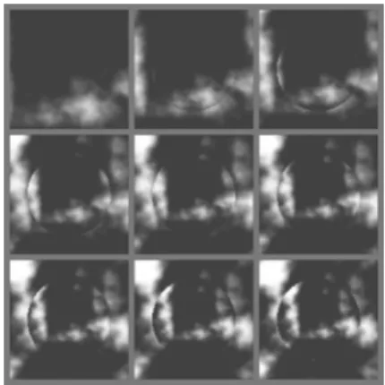
There is one problem with previously men-tioned paths – they are too regular to be natural. Smoke rising is rarely as perfect as a smooth he-lical path, although it manifests such behaviour at a large scale. Small-scale deviations are in-serted by means of a turbulent distortion that enhances animation veracity a great deal. A sample output of texture animator with per-turbed cycloidal path is:
// 6p are three periods of cycloid angle = 6 * PI * ntime
// move the point along the path, // move in z direction is linear P2 = transform("shader", P)
P2 -= (0.05 * (1 - 0.2 * cos(angle)), 0.05 * (fi - 0.2 * sin(angle)), -0.5 * ntime)
// add perturbation P2 += 0.05 * noise(P2)
An exemplary image sequence of animated flame texture is shown in fig. 1. The animation path is a vertical cycloid. Frames follow from top left to bottom right in rows.
Fig. 1.Animating flame by moving rendered points along cycloidal path.
shape and strength of attractor can vary over time, producing very practical animations. Again, spherical and linear attractors are eas-iest to do, while possibilities are almost unlim-ited(Ebert et al., 1994). Repulsorsare negative
attractors.
We have extended the texture animator to in-clude few primitive attractors/repulsors. Each
attractor is described by several characteristic parameters, such as centre point and radius for a spherical attractor. Each rendered point is moved in direction away from the closest point on the attractor, so that the visual effect is op-posite. The length of the move depends on the attractor strength and point-attractor distance. Fig. 2 is a sequence of frames showing the wide-angle objective effect of a strengthening circu-lar attractor/repulsor combination produced by
the following chunk of automatically generated code:
// circular attractor/repulsor is // described with its centre point // and radius
away = P-centre l = length(away)
// if inside the circle then // elongate the move
if (l<radius) away *= 2 // move the point
P2 = transform("shader", P) P2 += ntime*away
Fig. 2. Spherical attractor producing wide-angle objective effect.
2.2. Changing the texture space
Changing the texture space is probably the most natural way of texture animation. It requires di-rect modification of texture function core and thus necessitates its detailed knowledge. Tex-ture value is seldom calculated in one step, but rather gained by combining several quantities. Some of those quantities are given in parameter values and some are calculated separately. In the end, independent quantitiesqi may be
sim-ply added together to give the final texture value
T:
T =
X
i
wiqi (1)
Values wi are user-defined weights.
Normal-ized time component t can be comprised in calculation using any function f(t) that maps
range0,1]onto itself. Simplest cases of f are
f(t) = t and f(t) = 1;t. Texture evaluation
then sounds:
T =
X
i
wifi(t)qi (2)
Continuous mapping provided by functions fi
assures smooth texture animation.
Unfortunately, texture value is hardly ever pro-duced by a simple weighted summation. Par-ticipating quantities are usually interdependent. The extreme case would be if the amount of every quantity would influence the amount of next quantity, so the texture value would be the given by the following equation:
T =gn(gn ;1
ing various offsets, distortions and the like. Practical drawbacks of texture space animation are that it is not very intuitive and is also hard to automate, so texture animator is primarily used to insert typical cases of f functions.
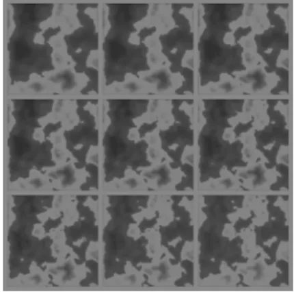
To demonstrate the richness and power of this technique, we have used a simplified version of fractal terrain generator(Musgrave et al., 1989).
Fig. 3 shows the image sequence of a develop-ing planet surface. Two quantities are bedevelop-ing regulated:
the amplitude multiplier in the fractal loop is linearly increased, causing the coastline to reshape and islands to appear and
the terrain altitude is evened out by a quadratic time function, producing the effect of vegeta-tion extincvegeta-tion.
Fig. 3.Development of planet texture with time-dependent texture function.
The relevant code reads:
alt = (1-ntime*ntime/2)
* fractal(P,8,2,0.5+(ntime*0.2))
colour mapping function transforms normalized texture values into colours usingcolour palette. Colour palette may contain arbitrary number of colours. For example, if colour palette contains 11 colours, then texture value 0.0 maps to the first colour, texture value 0.1 maps to second colour and so on. Texture value 1.0 maps to the last colour in the palette. Intermediate texture values map to colours that are interpolation of two corresponding colours from the palette. Such notion of colour mapping is in practice prevalent with mapping function being the in-terpolating curve, usually some sort of cubic colour spline(Musgrave, 1991). In spline
ter-minology the colours in the palette are called
knots. Spline-based colour mapping is particu-larly common in Renderman compliant shaders because the shading language directly supports cubic Catmull-Rom colour splines via built-in function calledspline.
Two different techniques can then be used to animate the texture:
changing the colour palette and changing the interpolating function.
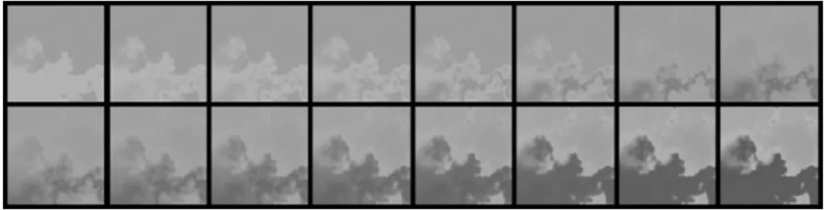
Fig. 4.Process of colour blending with time dependent colour palette.
time t is in case of linear palette interpolation given by:
Cti =(1;wifi(t))C
0
i +wifi(t)C
1
i (5)
Weights wi must all lie in the range 0,1] and
functions fimust be bijective on that range. All
power functions meet that condition.
Three or more colour palettes and another spline interpolation between them can supply addi-tional animating power. We emphasize that two interpolations are taking place here: interpola-tion of colour palettes and interpolainterpola-tion between colours in each palette.
Implementation of such scheme using the shad-ing language is very elegant:
Colour = spline(texturevalue,
pif1(f(ntime),colour11,,colour1i), pif2(f(ntime),colour21,,colour2i), ...
)
The outer spline function does the interpola-tion between colours in the palette. The latter are determined by inner interpolation functions, denoted bypifxabove. Depending on what kind of interpolation exists between colour palettes, functions mix, smoothstep or spline would be used in place ofpifxfor linear, cubic or general spline interpolation, respectively.
Second listed option is available with parameter-shapable interpolators. The simplest example is the Hermite spline that can be shaped by chang-ing tangent vectors in all points. Many variants of B-splines exist that can also be parametrically fine-tuned. Any such interpolating function can be used as long as it is reshaped in order to return colour values.
We have extended texture animator with colour mapping support routines. Up to four colour palettes may be constructed by visual picking up of colours and the desired interpolation scheme is built.
Fig. 4 shows phases of colour absorption pro-cess. The animation may not be extremely useful in this form but is typical for the tech-nique discussed here. The only thing changing is the colour palette of 10 colours. Fig. 5 shows apple ripening, attained by linear interpolation between colour palettes of four colours only. Richer collection of effects can be achieved with combinations of all mentioned techniques.
Fig. 5. Apple ripening with time dependent colour palette.
3. Conclusion
Texture animation has already proven its impor-tance in practice, but not all aspects of it have been presented here. Hypertextures(Perlin and
Hoffert, 1989)and other textures that are based
ture generation tools and specialized interfaces
(Worley, 1993).
References
1] D. S. EBERT, W. CARLSON, R. E. PARENT, Solid
Spaces and Inverse Particle Systems for Controlling the Animation of Gases and Fluids. The Visual Computer,10(1994), 179–190.
2] D. S. EBERT, F. K. MUSGRAVE, D. PEACHEY, K.
PERLIN, S. WORLEY, Texturing and Modeling – a
Procedural Approach, Academic Press, San Diego, 1998.
3] F. K. MUSGRAVE, C. E. KOLB, R. S. MACE, The
Synthesis and Rendering of Eroded Fractal Ter-rains, SIGGRAPH ’89 Proceedings, 23 (1989),
41–50.
4] F. K. MUSGRAVE, A Random Color Map
Anima-tion Algorithm, in Graphics Gems II, (1991) pp.
134–137, Academic Press, Boston.
5] K. PERLIN, E. M. HOFFERT, Hypertexture,
SIG-GRAPH ’89 Proceedings,23(1989), 253–262.
6] PIXAR,The Renderman Interface: Specification 3.2,
Pixar, San Rafael, 2000.
7] G. TURK, Reaction Diffusion Textures, Computer
Graphics,25(1991), 289–298.
8] S. WORLEY, Practical Texture Implementation,
Pro-cedural Modeling and Rendering Techniques course notes,ACM SIGGRAPH 1993,12.
Received:October, 2000
Accepted:November, 2000
Contact address:
Damjan Strnad Laboratory for Computer Graphics and Artificial Intelligence Department of Computer Science Faculty of Electrical Engineering and Computer Science University of Maribor Smetanova 17 SI-2000 Maribor, Slovenia phone:++386 62 220-7472
e-mail:[email protected]