Improving the Reliability of
Decision-Support Systems for
Nuclear Emergency Management by
Leveraging Software Design Diversity
Tudor B. Ionescu and Walter Scheuermann
Institut f¨ur Kernenergetik und Energiesysteme (IKE), Stuttgart, GermanyThis paper introduces a novel method of continuous ver-ification of simulation software used in decision-support systems for nuclear emergency management (DSNE). The proposed approach builds on methods from the field of software reliability engineering, such as N-Version Programming, Recovery Blocks, and Consensus Recov-ery Blocks. We introduce a new acceptance test for dispersion simulation results and a new voting scheme based on taxonomies of simulation results rather than individual simulation results. The acceptance test and the voter are used in a new scheme, which extends the Consensus Recovery Block method by a database of result taxonomies to support machine-learning. This enables the system to learn how to distinguish correct from incorrect results, with respect to the implemented numerical schemes. Considering that decision-support systems for nuclear emergency management are used in a safety-critical application context, the methods intro-duced in this paper help improve the reliability of the system and the trustworthiness of the simulation results used by emergency managers in the decision making process. The effectiveness of the approach has been assessed using the atmospheric dispersion forecasts of two test versions of the widely used RODOS DSNE system.
ACM CCS (2012) Classification: Information systems →Information systems applications→Decision sup-port systems→Expert systems
Keywords: software reliability, decision-support, simu-lation, safety-critical, machine-learning
1. Introduction
An atmospheric dispersion simulation code (ADSC) is a computer program, which imple-ments an atmospheric dispersion model(ADM).
In the aftermath of the Chernobyl nuclear acci-dent in 1986, atmospheric dispersion models and simulation codes were used to assess the radiological situation in Western Europe, which was one of the worst affected areas. On this occasion, at least two important aspects con-cerning ADMs and ADSCs became evident. Firstly, atmospheric dispersion models can be used for (1) assessing the radiological situa-tion any time after the release of nuclear trace species, (2) supporting decision-makers in the process of deciding upon and implementing ap-propriate counter-measures, such as the distri-bution of iodine tables or the evacuation of severely affected areas, while the accident is unfolding, and (3) training for nuclear emer-gencies (i.e., drills). These systems produce forecasts of the atmospheric dispersion of ra-dioactive materials using input data from var-ious sources, including nuclear power-plants, weather forecast centers, and radiological mea-surement stations. Dispersion forecasts are used by government emergency response committees and nuclear power-plant operators in preparing for and managing nuclear emergencies.
nu-clides. More recently, the European Commis-sion also funded a project, called ENSEMBLE [1] with the aim of developing a methodology for assessing the reliability of several medium and long-range atmospheric dispersion models currently in use in the European Union and other countries of the world. The outcome of this work was a multi-model approach, called en-semble dispersion modeling (EDM). The sys-tem aggregates results produced by different ADSCs implementing various models, and out-puts a unified result based on selecting the pth percentile result from the ensemble for each time step and each location of the monitored area.
1.1. Motivation
Germany, as well as other countries, in case of a significant release of radioactive materi-als into the atmosphere, the decision on which countermeasures to take and which sectors of the monitored area to evacuate first is taken based on these forecasts. Thus, simulation-based decision-support software systems must be regarded as safety critical. Therefore, it is necessary to investigate the reliability of such systems from a software reliability point of view. Section 4.1.1.2 of the NASA-STD-8719. 13B standard for safety-critical software[2] pro-vides a list of criteria for determining whether a software component or system must be con-sidered safety critical. Accordingly, it suffices for the software component in question to meet just one of the listed criteria in order for it to be regarded as safety critical. Paragraph 4.1.1.2.a. states that as soon as the software “processes data or analyzes trends that lead directly to safety decisions”, it must be considered safety critical. Moreover, note 4−1 from the same standard specifies that“if data is used to make safety decisions (either by a human or the sys-tem), then the data is safety-critical, as is all the software that acquires, processes, and transmits the data”. Decision support systems for man-aging nuclear emergencies(henceforth referred to as DSNE systems) are in use in all Euro-pean countries producing nuclear energy – see for example[1]for a comprehensive list. They are safety critical because erroneous dispersion simulation results could lead to false assump-tions about the dispersion of radioactive pollu-tants and may thus bias evacuation priorities.
1.2. Proposed Approach
Considering the simple fact that ensemble fore-casting systems are a paradigmatic example of the software design diversity principle, the pri-mary aim of this work is to assess the pos-sibility of detecting latent software faults in the dispersion models participating in ensem-ble forecasting systems using a new software design diversity method. The current approach helps improve the reliability of ADSCs by al-lowing the effective automated continuous ver-ification[3]of these simulation codes. The pro-posed approached is based on combining the N-Version Programming(NVP) [4]and Recov-ery Blocks(RB) [5]methods while developing a completely new voting scheme as well as a new acceptance test for dispersion simulation results.
The remainder of the paper is organized as fol-lows. We first briefly review the ADMs imple-mented in the RODOS system[6]and then pro-vide a literature review on verification methods for atmospheric dispersion simulation codes. We then review the current debate concerning software design diversity methods and argue that they are well suited for the case of dis-persion forecasting systems. We introduce a new acceptance test and taxonomy-based voter, which enable the application of the NVP and RB methods for the continuous verification of dispersion simulation codes. Finally, we evalu-ate the approach using two ensembles of artifi-cially generated data and discuss the results of the evaluation.
2. Materials and Methods
2.1. Atmospheric Dispersion Modeling
trace species. This property is an essential pre-requisite for the applicability of the software design diversity methods proposed in this work to the simulation codes implementing any of the models considered here.
2.1.1. The Gaussian Plume Model
The Gaussian Plume Model(GPM)is the old-est dispersion model with practical applicabil-ity. The model is based on an analytical solu-tion to the transport equasolu-tion, which accounts for the airborne transport of trace species. This transport occurs through the mean air flow(i.e., wind), in which case it is calledadvection, and through turbulent movement. Turbulence can disperse trace species in all three directions of space represented by the three axes of the Carte-sian system. This process is called diffusion. Any dispersion of substances which does not take place along the main flow is referred to as turbulent diffusion. The substances contained within an air volume are quantified by their con-centration per unit volume,c[kg m−3].
2.1.2. The Lagrangian Particle Model
The Lagrangian particle dispersion model (LPDM) [8]was adopted by the scientific com-munity and regulatory authorities by the end of the 90s as the field’s de facto standard[9]. The DIPCOT[10]simulation code, which is used in an operational DSNE system, represents an im-plementation of the Lagrangian particle model. In this model, an ensemble of particles is used to represent a much higher number of molecules of substance per particle released into the at-mosphere (i.e., trace species). The particles also reflect the physical properties of the trace species they stand for. The monitored area is divided into a 3-dimensional regular grid for which a wind field is computed at the begin-ning of each time step. Then, according to the wind velocity and direction, within one time step each particle can move from one grid cell to another whereby its location is updated. In addition to the change of position, the particle will suffer a change in its mass due to gravity (dry deposition) and/or precipitation(wet de-position). Through dry and wet deposition the air concentration of the trace specie(s) repre-sented by some particle will decrease according to first order differential processes.
2.1.3. Puff Models
Puff dispersion models are more accurate than Gaussian-Plume models and less time-consum-ing than the Lagrangian particle model. These models simulate the dispersion of trace species using a series of Gaussian puffs of different sizes. A puff contains a quantity of pollutant (characterized by its concentration) which is subject to turbulent diffusion and advection by a wind field in a way that is similar to how par-ticles are transported. RIMPUFF [11]and AT-STEP[12]are the two codes implementing puff models used to evaluate the current approach.
2.2. The Verification and Validation of Atmospheric Dispersion Simulation Codes
Much like any other software product, disper-sion simulation codes must undergo a thorough verification and validation phase prior to being integrated into production systems. [13] pro-vide an extensive overview of the best practices and methods for the verification and validation of simulation codes from the fields of compu-tational engineering and physics. According to[13], code to code comparisons are only ac-cepted as verification procedures provided that traditional and well accepted verification and validation procedures have been undertaken as well. An equivalent method to code to code comparisons has been used for comparing com-mercial seismic data processing software. In an extensive N-version programming study(called the T-experiments) [14], the authors show that the different versions of the scientific software participating to the study compared led to over-whelming disagreement between results due to software problems.
particle models only. That is, most of the tests cannot be applied to Puff models. Also, these tests can only be performed during the test and integration phase of the system because they re-quire extensive preparation, many repetitions, and qualitative assessment of the results. More-over, none of the tests can be easily automated. This makes them unsuitable for detecting er-rors in arbitrary dispersion simulation results produced by operational DSNE systems. In practice, the de facto standard method of ver-ification is that of plausibility checks through visual inspection.
In[15]the authors propose simple processes and tests for improving the reliability and usefulness of models, while in [16] which also provides a good review of other relevant work target-ing the software engineertarget-ing practices within the EMS community, the authors recommend a comprehensive 10-step development and eval-uation process for environmental models. Sci-entific software often has a lifetime of several decades and therefore the evolution of scientific software needs to be studied more thoroughly [17]. Different studies have pointed out that a quality-oriented software development culture may be considered less important in research institutes than model developments and refine-ments, considering that researchers are gener-ally more interested in producing and publish-ing state-of-the-art research results than high-quality software[14,18].
In [19] the authors define verification as “the determination that the code solves the chosen model correctly” and validation as “the deter-mination that the model itself captures the es-sential physical phenomena with adequate fi-delity”. The same authors further argue that ver-ification must always precede validation since otherwise any agreement between its results and experimental data is likely to be a product of chance.
In the field of atmospheric dispersion modeling, validation generally prevails over verification in most published studies. Perhaps, this is be-cause most codes are old and verification is usu-ally done only once in the early testing phase. Benchmarking (i.e., comparing the output of the code being verified to the outputs of well-established codes)is the most common verifica-tion method used in published work. Different
experimental data sets are also available from the HARMO website1 along with validation
and verification guidelines. Within the atmo-spheric dispersion modeling community there is a strong credo that verification must always imply comparisons with measurement data. In this context, considering that in software test-ing the aim is to also cover possibly unlikely input cases to the end of finding software faults, as for example in random testing [20], a para-dox becomes evident: while measurement data from experiments and accidents, such as the ones from Chernobyl and Fukushima, provide a gold standard for the evaluation of dispersion models, these datasets are limited in number. From a software testing perspective, this also limits the number and variety of input test cases considered for verification purposes. This prac-tice contrasts with the software testing princi-ples based on test case coverage criteria [21]. Test coverage criteria aim at stressing the limits of the software being tested to the end of find-ing more faults rather than makfind-ing the software behave as expected for a limited set of input cases.
In[22]and[17]the authors point out that there are very few published methods and studies aimed at finding and removing pure code faults (or mistakes) from scientific software. They propose a new type of testing activity, called code scrutinization, which is to be carried out before verification and validation. The authors show that random and mutation testing can suc-cessfully be used for code scrutinization. This white-box testing method is well suited for the developers of stand-alone dispersion simulation codes. However, for DSNE systems, which in-corporate several functionally redundant disper-sion simulation codes developed by different in-stitutes, the source code may not be available. Therefore, in the case of DSNE systems, most of the time only gray and black-box testing can effectively be carried out. The results of these testing activities are communicated to the devel-opers of the respective codes in the form of the input cases that triggered disagreement between the codes implemented in the DSNE system.
2.2.1. Validation and Benchmarking Studies with the RODOS System
The RODOS system encompasses three disper-sion codes-ATSTEP, DIPCOT, and RIMPUFF-developed at different research institutes around the world. RODOS is used in several Euro-pean countries(including Germany)as the offi-cial decision support system for nuclear disaster management. All three dispersion simulation codes used in RODOS have been subjected to validation using measurement data and to com-parisons with other systems [23,24,25,26]. In the most recent validation study targeting the codes used in the RODOS system based on inter-code comparisons and comparisons with experimental data the author states that “the models should deliver similar results under[the considered]circumstances,” while some results proved to be definitely wrong and some cases revealed significant discrepancies in the results of different models[27]. RODOS has also been evaluated using data from the Fukushima ac-cident and compared to other similar systems on the basis of the Fukushima case [28,29]. One study also discusses the modifications that needed to be made to the RODOS system in or-der to support several release phases spread over several weeks, as was the case of the Fukushima accident[30]. This type of release had not been foreseen by the creators of the system before the Fukushima accident.
After the Fukushima accident, a large bench-marking study which comprised 9 atmospheric dispersion models, including the three RODOS models, used in Germany and Switzerland has been carried out[31]. In this study, 8 artificially generated input cases starting from simple me-teorological conditions to realistic weather sit-uations were formulated to define the boundary conditions for the calculations. This experi-ment is noteworthy not only because it uses many atmospheric dispersion codes, but also because 7 of the 8 input cases are artificially generated. Only one case, deemed more realis-tic by the authors, uses weather data predicted by the COSMO model of the German Weather Service.
All these studies show that, while RODOS is a well-regarded validated DSNE system, there are improvements to be made whenever a new data set becomes available or new codes are used in the comparison. This underpins the idea
that continuous verification and better test cov-erage, which also includes unlikely input cases, can only improve the system over time.
2.3. Multi-Model Ensemble Forecasting Systems
Multi-model ensemble dispersion forecasting systems represent the state of the art approach in the ensemble dispersion forecasting commu-nity. In this approach, several functionally re-dundant simulation codes are used to produce an aggregated result, which is in fact selected using a voting scheme. While there is consen-sus in the community that ensemble systems produce better results than single version sys-tems [32], there is a lively debate in literature about how to identify the models, which have a bad influence on the other members of the ensemble to the end of using a more reliable reduced ensemble of models. One strategy is to eliminate those results from aggregation which are deemed redundant with respect to their bias [33]. This strategy contrasts with the software design diversity principle discussed in the next section of this paper. Current best practices in multi-model dispersion forecasting ensembles suggest that model diversity and accuracy are key to providing more realistic and trustwor-thy results [34]. Here diversity is believed to be beneficial within a reduced ensemble when it produces a better result with respect to the gold standard (i.e., measured data). However good diversity relies on the accuracy of individ-ual models, which must be assessed beforehand. The reduced ensemble approach is complemen-tary to the weighting approach, where the results of all ensemble members are weighted prior to being used in computing an aggregated result [35].
2.4. Software Design Diversity
has been argued that failure correlation strongly depends on the application of software engi-neering methods and best practices during the software development process, hence, the possi-bility of reducing the probapossi-bility for failure cor-relation by improving the software development processes [38]. In [39]the authors proposed a model for why different developer teams tend to make the same mistakes based on the notion of “variation of difficulty” over the demand space. This model states that greater variation of diffi-culty increases the failure dependence between functionally redundant software versions. An-other approach is to force diversity into the de-velopment process of the different versions – an approach which has been used for the Airbus A320 flight control software[40].
Currently, software design diversity methods are generally considered to improve the overall reality of the system, albeit at a cost that cannot be easily determined a priori[41]. The ongoing debate concerning the effectiveness of software design diversity is focused on the costs it in-volves over the costs of developing a reliable single version system [42]. In the case of at-mospheric dispersion forecasting software, the cost issue is not at stake because dozens of inde-pendently developed simulation codes already exist and have been integrated in ENSEMBLE systems. Here, the problem lies in the way that simulation results are being compared.
Once several functionally redundant versions, of a program are available, it is possible to de-velop a new software design diversity method based on existing patterns from the domain of software reliability engineering, such as Recov-ery Blocks(RB) [5]or N-version programming (NVP) [43]. Such methods require an accep-tance test and a voting scheme, both of which will be introduced in the following sections.
2.5. A New Acceptance Test for Atmospheric Dispersion Simulation Results
The acceptance test proposed in this paper can be regarded as both an accounting check and a reasonableness test – see[44]for a classification of acceptance tests. The acceptance test checks that the distribution of the frequency function of all concentration or dose values obtained by dropping the spatial information from the
dataset(i.e., by converting 2 and 3-dimensional matrices into one dimensional arrays of values) obeys a certain hypothetical distribution. The frequency function is obtained by generating a histogram of the values for all cells of the dis-cretized monitor area. Using simple input cases for which the activation of software faults is highly unlikely, we found that the hypothetical frequency function has the shape of the Weibull distribution [45], as also noted in [46]. Intu-itively, this means that (1) in any dispersion simulation result, the number of high concen-tration values must be much smaller than the number of low concentration values and(2)that the transition from one concentration level to another must be smooth and gradual. This rep-resents the hypothesis of the proposed accep-tance test, which was implemented in R2. After
reducing the two-dimensional matrix contain-ing the concentration or dose values to a one-dimensional array(i.e., dropping the spatial in-formation from the dataset) a goodness of fit test can be used with the resulting data set. The Kolmogorov-Smirnov goodness of fit test [47] proved to be suitable for an automated accep-tance test for several reasons. The Kolmogorov-Smirnov (KS) test is a distribution-free good-ness of fit test, which tests whether or not an em-pirical cumulative distribution function(CDF) fits a hypothetical(expected) CDF. Compared to other statistics, the KS test is more intuitive and easier to implement. Simplicity is a desir-able property of an acceptance test in a soft-ware reliability engineering sense. It also uses the empirical and hypothetical CDFs functions directly rather than contingency tables. Also, the hypothetical distribution of the concentra-tion and dose values was unknown to us when we started the tests and, in theory, the KS test works with any hypothetical distribution. Fi-nally, not as much emphasis was put on the selection of a particular statistical test as on the pragmatic implementation considerations. Any goodness of fit test that works with this kind of data and requires a simple implementation can be used.
Since the Weibull distribution is L-shaped it makes the application of an automated goodness of fit test difficult(in an L-shaped histogram the vast majority of the measurements fall into the first interval from the left). To overcome this
inconvenience, Weibull-distributed data sam-ples can be transformed into exponentially dis-tributed samples before applying the goodness of fit test. The transformation of the data set prior to applying a goodness of fit test is very common in the statistical practice[48].
2.6. A New Taxonomy-Based Voter for Atmospheric Dispersion Simulation Results
One way of obtaining taxonomies from arbi-trary data is through hierarchical clustering[49]. Hierarchical clustering has an important advan-tage over other clustering methods(such as par-titional clustering); namely, it allows for ex-act comparisons between resulting taxonomies. By relating new results to existing ones, a tax-onomy of intra-model results can be obtained. By intra-model results it is meant that all re-sults participating to the test are produced by the same dispersion simulation code. The tax-onomy represents the memory (or history) of the dispersion code whereas the process of clas-sifying a new result into an existing taxonomy may be regarded as a learning process. The most important thing here is to be certain that new results which are to be incorporated into a taxonomy (i.e., what is being learned) are not flawed; for, once accepted in the taxonomy, they are taken to be correct.
2.6.1. A New Metric for Atmospheric Dispersion Simulation Results
Ametricis a functionddefining a distance be-tween arbitrary individuals from a population. A data set with an associated metric is called a metric space and is denoted by (M,d). Dis-persion simulation results are provided in form of two or three-dimensional matrices whereby each matrix element corresponds to one area or volume element of the regular grid used to discretize the monitored area. The values con-tained in these matrices can be provided in ar-bitrary units. In the case of radioactive trace species, the values corresponding to each grid cell can be one of integrated activities/doses or as activity/dose rates expressed in either [Bq] (Bequerel) / [Sv] (Sievert) or [Bq] / [Sv] per unit of time.
Dispersion plumes can be regarded as distribu-tions of continuous variables in a finite space
delimited by the monitoring area. In this case the residual sum of squares(RSS)can be used as a metric on the result space by letting one of the plumes account for the observed valuesyi and the other one for the estimated valuesf(xi):
RSS=ni=1[yi−f (xi)]2. (1)
The normalized version of the RSS metric can be used with the results of arbitrary dispersion codes, since all of them produce matrix-based outputs. The use of a normalized metric also guarantees that the distances between arbitrary result spaces will be preserved(i.e., isometry). Since dispersion simulations are iterative, af-ter each time step a new result matrix becomes available. When comparing intra-model results, one can choose to include any number of time steps in the calculation of the normalized RSS metric. In statistics it is common practice to per-form transper-formations on the data prior to analyz-ing them. In the case of dispersion simulation results, applying a power transformation with a power 0 < p < 1 will smoothen and level the data since very large values will become smaller and sub-unitary values will increase. Given a power 0 < p < 1 and two dispersion simula-tion resultsr1andr2defined on anN byMcell
monitored area for a number of TStime steps, the generalized RSS distance is given by:
GRSS(r1,r2)=
i≤TS
t=1
i≤N
i=1
j≤M
j=1(r1[t,i,j]
p−r2[t,i,j]p)2
(2)
The advantage of this metric over other metrics is that it provides a high level of flexibility by letting the practitioner select the most suitable value ofp.
2.6.2. The Reference Input Case Ensemble
The reference input case ensemble will serve as the basis for the evaluation of the methods in-troduced in this work. The main requirements to the reference input case ensemble are the fol-lowing:
− It shall cover the entire monitored area sur-rounding the chosen point of emission;
(WD), wind speed(WS), accident category (AC), and diffusion category(DC);
− The variation shall be equidistant(where ap-plicable);
− The wind direction shall be varied such that neighboring plumes overlap to some extent;
− The number of simulation steps and the sim-ulated time shall not be varied from one input case to another.
The “each-used” test case coverage criterion [21] yielded the list of input cases shown in Figure 1. The names of the cases are coded as follows: the first letter represents the turbulent diffusion category(A to F), the next three digits represent the wind direction, the number fol-lowing the letter ‘S’ stands for the wind speed in m/s, and the number following the letter ‘F’ represents the release(or accident)category ac-cording to the DSRA risk study [50]. Table 1 contains information about the amount and type of radioactive substance that is released into the atmosphere depending on the release category. The categories are ordered with respect to the total activity of the released radionuclides. In consideration of the previously stated require-ments to the reference input case ensemble, the point of emission was chosen to be the KKP-2 (Philippsburg 2)reactor in Germany and the radius of the monitored area 16 km. The area surrounding the Philippsburg 2 reactor is rather flat, so the topography of the monitoring area does not have great influence. The simulation duration was chosen to be 2 hours divided into 12 time steps of 10 minutes each. The time win-dow of 2 hours was chosen in accordance with
Figure 1.Sketch of the reference input ensemble.
the modeling area of 16 km in radius, which is also within the scale of the Fukushima evacua-tion area. At the highest considered wind speed of 8 m/s(28.8 km/h), the trace species emit-ted at t = 0 would reach the boundary of the modeling area in less than 30 minutes. This is sufficient to activate software faults related to erroneously posed boundary conditions, which may occur after part of the trace species exit the monitoring area. Ill-posed boundary conditions can lead to a violation of the mass conserva-tion principle. This principle is fundamental in the numerical simulation of partial differen-tial equations, such as the transport equation, and thus provides a suitable verification crite-rion. The data used in the reference input case ensemble are generated using the meteorologi-cal preprocessor of the RODOS system and are thus artificial. It is a common practice in run-ning “what if” simulation scenarios for users of
Table 1.The eight release categories and corresponding amounts of radioactive materials with respect to the total amount present in the reactor according to the DSRA risk study[50]. A star marks the release categories
corresponding to core meltdown accidents.
Release category
Emission height
[m]
Duration
[h] gas [%]Noble Iodine[%] Alkali metals [%]
Tellurium / Antimony
[%]
Alkaline earth metal [%]
Ruthenium group
[%]
Lanthanides [%]
F8 100 6 0.02 0.00 0.00 0.00 0.00 0.00 0.00
F6* 100/10 3 2.30 0.00 0.00 0.00 0.00 0.00 0.00
F5* 10 3 2.30 0.11 0.07 0.07 0.01 0.01 0.01
F7 10 1 1.70 0.53 1.30 0.00 0.00 0.00 0.00
F4* 10 3 66.80 1.47 0.34 0.33 0.04 0.33 0.00
F3* 10 3 66.80 4.68 2.93 2.67 0.33 0.22 0.03
F2* 10 3 66.80 27.12 19.32 12.68 2.31 1.13 0.17
the system to manually input the wind speed and direction, as well as the precipitation rate and the turbulence parameters.
The released activity which is given by the re-lease category is taken into account when com-puting the GRSS metric for two arbitrary disper-sion simulation results. Thepparameter of the GRSS metric allows one to control the influence (or weight) of the amount of released activity (i.e., concentration of substance)upon the ref-erence taxonomy of results. For 0.4 > p > 1, the weight of the activity is greater than that of the wind direction. It is therefore justified to vary the release categories, and thus the amount of released activity among the input cases from the reference ensemble.
2.6.3. The Reference Taxonomy of Results
Considering a set of N intra-model dispersion simulation results (henceforth called ensemble of results), a distance matrixD is obtained by computing all possible distancesdijbetween all
result pairsij. The distances are computed us-ing the GRSS metric. Startus-ing from the distance matrixD, a multitude of clustering methods can be used to build a taxonomic scheme of disper-sion simulation results.
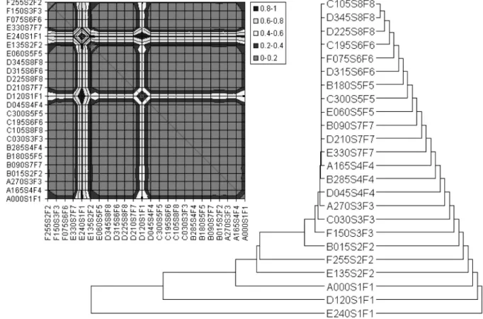
Figure 2 shows the surface plot of the 24 by 24 distance matrix corresponding to RIMPUFF results for the ensemble of 24 input cases in-troduced in the previous section as well as the taxonomy of results inferred by means of the centroid method. The results represent the time-integrated near-ground gamma sub-mersion dose. The distances have been com-puted using the GRSS metric(forp =1)for all 12 time steps accounting for a 2-hour simula-tion. The results taxonomy is represented as a phylogram. The lengths of the branches in the left hand side phylogram reflect the distances between the elements being clustered as pro-vided in the distance matrix. By contrast, the branch lengths of the phylogram on the right-hand side do not reflect the original distances from the matrix. Instead, this one’s purpose is to show the topology of the taxonomic tree.
Figure 2.Surface plot of a 24×24 distance matrix computed from RIMPUFF results for the 24 input case reference ensemble, as well as the corresponding taxonomic tree built by means of the centroid method. The taxonomy is
The phylogram has the topology of a caterpil-lar tree which reflects the order relations within the sample. The results are first ordered by the amount of the released radioactive materi-als specified by the release category (denoted “F1” to “F8” in the names of the input cases). The second ordering criterion appears to be the atmospheric stability class.
2.6.4. Comparing Taxonomies of Results
Dispersion simulation codes fulfill the two ba-sic requirements of the N-version programming paradigm: (1) they are developed and main-tained by completely independent developer teams, and(2)they implement dispersion mod-els which all approximate the solution to the transport equation. Hence, they start from the same basic functional requirement – solving the transport equation numerically. However, due to the inherent differences in the numerical schemes used for solving the transport equa-tion, the results of the various dispersion codes will differ to such an extent that finding suitable thresholds and tolerance values to be used by voters can be rather difficult.
The aim of the current approach is to assess the degree of similarity (or dissimilarity) between the results of two or more arbitrary dispersion codes C1. . .Cn by first constructing a taxon-omy of results for each of them starting from the same ensemble of input casesP={p1, . . . ,pn} and then by comparing the resulting taxonomies rather than individual results. Using P as the input case ensemble, each dispersion code Ck will produce an ensemble of results R(Ck) =
{r1(Ck), . . . ,rn(Ck)}, whereby pi corresponds to ri(Ck) for i = 1, . . . ,n. The next step is to build taxonomic trees for each result ensemble. In order to build a taxonomy T{R(Ck)} from the members of some result ensemble R(Ck), the pair-wise distances between all of its mem-bers need to be computed using the metric of choiced which gives a distance(or dissimilar-ity)matrixD(Ck) = [di,j]fori,j= 1, . . . ,n, as described in the previous section. In this con-text, what enables the implementing voters is the following conjecture:
If C1 and C2 are two dispersion simulation
codes correctly implementing arbitrary numer-ical schemes for solving the transport equation,
then there exists a distance metric di,j defined on the metric space (M,d) of the dispersion sim-ulation results produced by C1and C2such that
T{R(C1)} ≡T{R(C2)}.
A dispersion code is considered to correctly im-plement a numerical scheme for solving the transport equation if and only if it conserves its mathematical properties (i.e., determinism, strict monotonicity, and continuity). Failing to do so is taken to be an indication of the presence of residual software faults in the code caused by the misinterpretation of the model or some other programming or computing error. The same principle applies to post-processing steps, such as the gamma submersion and effective dose calculation. Assessing the similarity be-tween taxonomic trees requires a metric defined on the tree space. The Robinson-Foulds(RF) symmetric difference [51] between two taxo-nomic trees counts the number of branches in the first tree which are not present in the second tree plus the number of branches in the second tree which are not present in the first tree. For a tree of N leaves, the maximal RF distance is 2N-4 if the trees are rooted and 2N-6 otherwise.
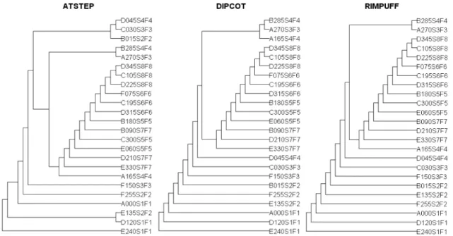
Figure 3 shows the taxonomic trees correspond-ing to the three codes implemented in the RO-DOS system. The RF distances between these trees are as follows(values in brackets represent percentages from the maximum RF distance for N =24):
• ADGRSS(p=0.6) =RF(ATSTEP,DIPCOT,
p=0.6) =16(38%),
• ARGRSS(p=0.6) =RF(ATSTEP,RIMPUFF,
p=0.6) =16(38%), and
• DRGRSS(p=0.6) =RF(DIPCOT,RIMPUFF,
p=0.6) =4(9.52%).
Figure 3.Taxonomic trees corresponding to the three dispersion codes implemented in RODOS. The trees were constructed by means of the GRSS distance withp=0.6.
2.7. New Software Design Diversity
Method for the Continuous Verification of Simulation Results
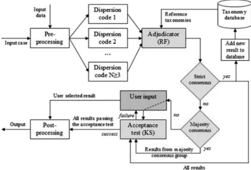
The workflow supporting the continuous verifi-cation of dispersion simulation results depicted in Figure 4 is based on the consensus recovery block algorithm[52], which combines the NVP and Recovery Block methods in one module. The novelty of the proposed method consists in using a database of result taxonomies in order to enable a machine learning process.
The method works as follows: the preprocess-ing step in the workflow from Figure 4 involves all computations which are usually required for preparing a dispersion simulation (wind and precipitation field computation, source term cal-culation, etc.) After preprocessing the input case and data, the simulation is performed by two or more functionally redundant dispersion codes. The adjudicator receives the results from allN ≥3 dispersion codes and fetches the refer-ence taxonomies corresponding to each of them from the database; then, it computes the dis-tance between the new result and the ones in the reference ensemble and reconstructs the taxo-nomic trees starting from the extended distance matrix. The new result is now regarded as a member of the reference ensemble. Next, the adjudicator computes the RF distance between the extended taxonomic trees. The following situations can arise:
- Strict consensus: the RF distances between all taxonomic trees are zero. All results are subjected to an acceptance test. The results passing the acceptance test are forwarded for post-processing;
- Majority consensus: the RF distance is zero within a group containing (N/2 +1) taxonomic trees (called majority consensus group). Only the results in the majority con-sensus group are subjected to an acceptance test. The results passing the acceptance test are forwarded for post-processing;
- Disagreement: consensus groups only con-tainN/2 or fewer trees. The user is informed about the disagreement and is asked to make a decision as to which result to take into consideration. This can be done by visual inspection, by analyzing the placement of the new results in the taxonomic trees, or by subjecting all results to the acceptance test.
Figure 4.Workflow for a dispersion forecasting system supporting functionally redundant simulation codes and continuous verification of results.
and RIMPUFF is given byCAL (ATSTEP, DIP-COT, RIMPUFF) = (20*100) / 24 = 83.33%. The sub-tree that is identical for all participat-ing codes will be referred to as the consensus tree (or taxonomy).
Continuous verification is achieved by imple-menting the tasks depicted in Figure 4 in the dispersion simulation workflow. Whenever a new simulation is carried out using 2 or more simulation codes, the results are added to the result taxonomies of each code stored in the tax-onomy database in Figure 4. This way, for each new result the user can be informed whether or not the new result leads to more disagreement among the simulation codes(i.e., by computing the CAL metric). If it does, the user can mark and comment the input case for further investi-gation by the creators of the simulation codes in question. Thus, the system helps identify input cases, which might reveal software faults upon a more detailed investigation. The results that do not lead to more disagreement between the codes are permanently added to the reference taxonomy database.
3. Experimental Validation
of the Approach
In order to validate the Kolmogorov-Smirnov acceptance test(KS-AT)and the
result-taxono-my-based voter for dispersion simulation re-sults, two versions of the RODOS decision sup-port system have been used. In the following, these two test versions of the system will be referred to as RODOS v1 and RODOS v2, re-spectively. Taking into account that each code implements a different numerical scheme, the RODOS systems is suitable for proving the va-lidity and practical applicability of the conjec-ture from section 2.6.4 and its implications. An-other argument in favor of this choice is the fact that RODOS is being used in several Eu-ropean countries (including Germany) as the official decision support system for nuclear dis-aster management[53]. The tests using the first version of the RODOS system revealed a num-ber of flaws in the results produced by the three dispersion codes implemented in the RODOS system, notably:
- The gamma dose levels computed by all three RODOS dispersion codes is not invari-ant with respect to the wind direction even when the topology of the monitored area is leveled;
- For certain input cases, ATSTEP yields zero-level gamma doses for the first few time steps despite that radioactive materials were re-leased in that time as well;
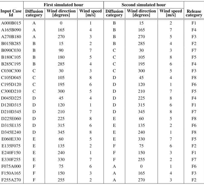
On the basis of these results the developers of the RODOS system admitted to have identified a fault in the ATSTEP dispersion code and car-ried out improvement works which concerned DIPCOT as well. These works eventually lead to a new release of the system(i.e., RODOS v2) which was afterwards made available to the au-thors. Using the two versions of the systems the exact same set of simulations has been carried out. These simulations were performed using two input case ensembles. The first one is rep-resented by the reference input case ensemble introduced earlier in this work. The second in-put case ensemble that was used is summarized in Table 2. It contains 24 input cases which rep-resent random combinations of the 24 reference input cases. Two simulated hours are divided
in 12 ten-minute time steps. After one simu-lated hour, the wind direction and speed change while all other parameters stay the same. Us-ing a second input case ensemble with varyUs-ing wind direction is motivated by the problems that dispersion models typically exhibit in rotating wind situations.
For both versions of the system, the correspond-ing reference taxonomy was used to verify the input cases from the second input case ensem-ble described in Taensem-ble 2. Each input case from this ensemble was regarded as a new simulation result to be verified given the existing opera-tional taxonomy. The procedure employed for accomplishing this task is the one depicted in Figure 4.
Table 2.The second input case ensemble with varying wind speed, direction, and diffusion category.
First simulated hour Second simulated hour Input Case
Id Diffusioncategory Wind direction[degrees] Wind speed[m/s] Diffusioncategory Wind direction[degrees] Wind speed[m/s] categoryRelease
A000B015 A 0 1 B 15 2 F1
A165B090 A 165 4 B 165 7 F4
A270B180 A 270 3 B 270 5 F3
B015B285 B 15 2 B 285 4 F2
B090C030 B 90 7 C 30 3 F7
B180C105 B 180 5 C 105 8 F5
B285C195 B 285 4 C 195 6 F4
C030C300 C 30 3 C 300 5 F3
C105D045 C 105 8 D 45 4 F8
C195D120 C 195 6 D 120 1 F6
C300D210 C 300 5 D 210 7 F5
D045D225 D 45 4 D 225 8 F4
D120D315 D 120 1 D 315 6 F1
D210D345 D 210 7 D 345 8 F7
D225E060 D 225 8 E 60 5 F8
D315E135 D 315 6 E 135 2 F6
D345E240 D 345 8 E 240 1 F8
E060E330 E 60 5 E 330 7 F5
E135F075 E 135 2 F 75 6 F2
E240F150 E 240 1 F 150 3 F1
E330F255 E 330 7 F 255 2 F7
F075A000 F 75 6 A 0 1 F6
F150A165 F 150 3 A 165 4 F3
3.1. Results
For each version of the RODOS system the KS test was first run on the basis of the two in-put case ensembles. The KS test can be ap-plied at a significance level(alpha)0.01, 0.05, 0.1, 0.15, etc. In practical terms, using al-pha=0.01 provides a less strict assessment than using alpha=0.05. Tests using alpha=0.05 lead to the rejection of more input cases than for al-pha=0.01 and it would have been more difficult to find correlations between the output of the voter and that of the acceptance test. However, we do recommend using a significance level of 0.05 if a more scrutinizing assessment of the trustworthiness of simulation results is aimed at, especially when the number of passing cases is getting closer to 100%.
The results of these tests are summarized in Ta-ble 3 (figures in boldface indicate an improve-ment from one version of the simulation code to another). They show that the KS test is sensitive to the improvements brought to the RODOS v2 system. The only exception is produced by the DIPCOT simulation code for the reference in-put case ensemble. In this case, the develop-ers might have introduced a new fault while attempting to correct others. Notably, the net improvement of ATSTEP v2 over ATSTEP v1 reflects the efforts of the developers to remove the flaws revealed by our previous verification analysis of the system.
Next, the consensus taxonomies for the two ver-sions of the systems were inferred on the basis on the reference input case ensemble. This is a prerequisite for performing the tests on the input case ensemble with rotating wind direc-tion. This yielded a 20-leaf consensus tree for the RODOS v1 simulation codes and a 21-leaf
consensus tree for the RODOS v2 simulation codes. In other words, the consensus agreement level for the two versions of the system wasCAL (ATSTEP v1,DIPCOT v1,RIMPUFF v1) = 83.33% and CAL (ATSTEP v2,DIPCOT v2, RIMPUFF v2) =87.5%, respectively.
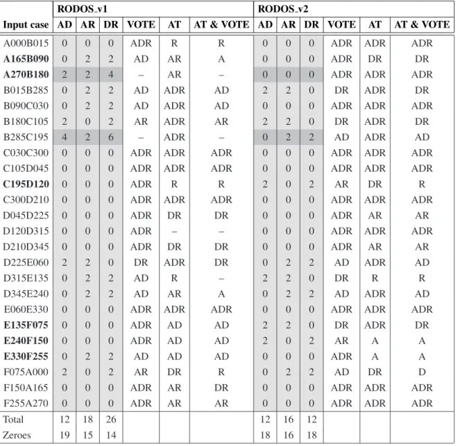
These high consensus agreement levels them-selves support the argument that the conjecture from section 2.6.4 holds for the dispersion codes implemented in both versions of the RODOS system. Moreover, the increase in the consen-sus agreement level between the codes from the second version of the system provides evidence that the CAL metric is sensitive to the removal of software faults from the simulation codes under investigation. Table 4 summarizes the consensus recovery block’s output for the re-sults of the two versions of the RODOS system for the 24 input cases from the test ensemble with varying weather conditions. In order to ensure equity for the comparison, an 18-taxon consensus tree(i.e., a sub-taxonomy of the con-sensus trees corresponding to the two versions of the system)correlated with the Kolmogorov-Smirnov test results was used with both versions of the RODOS system. The taxonomy based voter output clearly reveals an improvement of RODOS v2 over RODOS v1. While the to-tal RF distance for the pair ATSTEP-DIPCOT (AD)remains constant from one version to an-other, the pairs ATSTEP-RIMPUFF (AR) and DIPCOT-RIMPUFF (DR) yield smaller total RF distances (i.e., summed up over all input cases). The improvement for the pair DR is quite significant. While the improvements brought to the ATSTEP code were clearly re-flected by the KS test results, the smaller to-tal RF distance for the pair DIPCOT-RIMPUFF reflects the improvements in DIPCOT v2 over DIPCOT v1.
Table 3.Kolmogorov-Smirnov test results for the two input case ensembles for RODOS v1 and RODOS v2.
Reference Input Case Ensemble
α =1% ATSTEP v1 ATSTEP v2 DIPCOT v1 DIPCOT v2 RIMPUFF v1 RIMPUFF v2 Passed 16/24 22/24 20/24 19/24 21/24 21/24
Percent 66.67% 91.67% 83.33% 79.17% 87.50% 87.50%
Second Input Case Ensemble
α =1% ATSTEP v1 ATSTEP v2 DIPCOT v1 DIPCOT v2 RIMPUFF v1 RIMPUFF v2 Passed 17/24 20/24 15/24 19/24 20/24 23/24
Table 4.The strict consensus recovery block output for the 24 input cases with varying weather conditions for RODOS v1 and RODOS v2. Abbreviations: AD=RF(ATSTEP, DIPCOT); AR=RF(ATSTEP, RIMPUFF); DR=RF(DIPCOT, RIMPUFF); RF=Robinson-Foulds distance; VOTE=output of the taxonomy based voter for some given input case; AT=results of the Kolmogorov-Smirnov acceptance test; AT&VOTE=intersection of AT and VOTE output sets; A=ATSTEP; D=DIPCOT; R=RIMPUFF; Zeroes=number of input cases
for which the RF distance between the respective two simulation codes is zero.
RODOS v1 RODOS v2
Input case AD AR DR VOTE AT AT & VOTE AD AR DR VOTE AT AT & VOTE A000B015 0 0 0 ADR R R 0 0 0 ADR ADR ADR
A165B090 0 2 2 AD AR A 0 0 0 ADR DR DR
A270B180 2 2 4 – AR – 0 0 0 ADR ADR ADR B015B285 0 2 2 AD ADR AD 2 2 0 DR ADR DR B090C030 0 2 2 AD ADR AD 0 0 0 ADR ADR ADR B180C105 2 0 2 AR ADR AR 2 2 0 DR ADR DR B285C195 4 2 6 – ADR – 0 2 2 AD ADR AD C030C300 0 0 0 ADR ADR ADR 0 0 0 ADR ADR ADR C105D045 0 0 0 ADR ADR ADR 0 0 0 ADR ADR ADR
C195D120 0 0 0 ADR R R 2 0 2 AR DR R C300D210 0 0 0 ADR ADR ADR 0 0 0 ADR ADR ADR D045D225 0 0 0 ADR DR DR 0 0 0 ADR AR AR D120D315 0 0 0 ADR – – 0 0 0 ADR ADR ADR D210D345 0 0 0 ADR DR DR 0 0 0 ADR AR AR D225E060 2 2 0 DR ADR DR 0 2 2 AD ADR AD
D315E135 0 2 2 AD R – 2 2 0 DR R R
D345E240 0 2 2 AD AR A 0 2 2 AD ADR AD E060E330 0 0 0 ADR ADR ADR 0 0 0 ADR ADR ADR
E135F075 0 0 0 ADR AD AD 2 2 0 DR ADR DR
E240F150 0 0 0 ADR AD AD 2 0 2 AR A A
E330F255 0 2 2 AD AD AD 0 0 0 ADR A A F075A000 2 0 2 AR DR R 0 2 2 AD DR D F150A165 0 0 0 ADR AR DR 0 0 0 ADR ADR ADR F255A270 0 0 0 ADR AR AR 0 0 0 ADR ADR ADR
Total 12 18 26 12 16 12
Zeroes 19 15 14 18 16 18
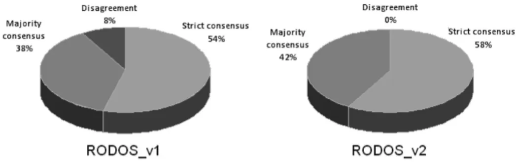
Figure 5 shows the exact percentages of the cases when each of the three possible outcomes (i.e., strict consensus / majority consensus / disagreement) is produced by the taxonomy-based voter for RODOS v1 and RODOS v2. Thanks to removing some of ATSTEP’s and DIPCOT’s software faults, the results for RO-DOS v2 no longer yield any cases of disagree-ment. The 8% disagreement share is split up in two fractions; one of them is gained by the strict consensus share, and the other one by the
majority consensus share. There also appears to be no improvement/deterioration pattern for the voter’s output except for the absence of dis-agreement cases from RODOS v2’s results. Figure 6 shows the percentage ratios of the 4 possible output types of the consensus recov-ery block(i.e., AT&VOTE column in)for both versions of the system:
Figure 5.Strict consensus/majority consensus/disagreement percentage ratios resulting from the taxonomy-based voter for the two RODOS versions for the 24 input cases with varying weather conditions.
Figure 6. Consensus/2 out of 3/1 out of 3/disagreement percentage ratios resulting from the output of the consensus recovery block(i.e., AT&VOTE column in Table 4)for the two RODOS versions for the 24 input cases
with varying weather conditions.
- 2 out of 3(labels “AD” for the pair ATSTEP-DIPCOT, “AR” for ATSTEP-RIMPUFF, and “DR” for DIPCOT-RIMPUFF): the results from two out of three codes are forwarded for post-processing;
- 1 out of 3(labeled “A” for ATSTEP, “D” for DIPCOT, and “R” for RIMPUFF): the result from one out of three codes is forwarded for post-processing;
- Disagreement(labeled “–”): the result from none of the codes is automatically forwarded for post-processing. The user is asked to make a decision.
Once again, for RODOS v2 the consensus re-covery block’s output does not yield any cases of disagreement. For RODOS v2, in 79.17% of the cases the user gets a consensual or “2 out of 3” recommendation from the system. This pos-itive evolution for RODOS v2 is due to a better correlation of the voter’s output with the ac-ceptance test results compared to RODOS v1’s case.
4. Conclusion
existence of latent software faults in simula-tion codes. The proposed approach thus helps finding further latent software faults in existing DSNE systems, such as the RODOS and the ENSEMBLE systems.
Considering that real data is the only gold stan-dard in the evaluation of atmospheric dispersion simulation software, we intend to repeat the ex-periment using the post-Fukushima version of the RODOS and possibly other systems based on a reference input case ensemble, which in-cludes the Fukushima data sets. For example, input case ensembles can be generated by vary-ing different parameters of the Fukushima data set. Such a study builds upon the approaches used in[31]and[30], while providing additional means for the application of verification crite-ria (such as the Gaussian boundary condition, the mass conservation principle, etc.) using the methods introduced in this work.
References
[1] S. Galmariniet al., “Ensemble dispersion forecast-ing, Part I: concept, approach and indicators”, At-mospheric Environment 38, pp. 4607–4617, 2004. http://dx.doi.org/10.1016/j.atmosenv.2004.05.031 [2] N. A. a. S. A. NASA, “NASA Standard for Software
Assurance (NASA-STD-8739.8)”, NASA, Wash-ington, D.C., 2004.
[3] P. E. Farrell et al., “Automated continuous ver-ification for numerical simulation”, Geoscientific Model Development, vol. 4, pp. 435–449, 2011. http://dx.doi.org/10.5194/gmd-4-435-2011
[4] A. Avizienis and J. C. Laprie, “Dependable com-puting: From concepts to design diversity”, Pro-ceedings of the IEEE 74, 1986, pp. 629–638. http://dx.doi.org/10.1109/PROC.1986.13527 [5] T. Anderson and R. Kerr, “Recovery blocks in
action: A system supporting high reliability”, in
Proceedings of the 2nd international conference on Software engineering, Los Alamitos, 1976. [6] J. Ehrhardt and A. Weis, “RODOS: Decision
Sup-port System for Off-site Nuclear Emergency Man-agement in Europe”, Directorate-General for Re-search, European Commission, Luxemburg, 2000. [7] D. Etling, “Theoretische Meteorologie”,Eine
Ein-fuhrung, Berlin-Heidelberg: Springer-Verlag, 2008.
[8] D. Etling et al., “Application of a random walk model to turbulent diffusion in complex ter-rain”, Atmospheric Environment, vol. 20, pp. 741–747, 1986. http://dx.doi.org/10.1016/ 0004-6981(86)90188-5
[9] Verein Deutscher Ingenieure, “Environmental me-teorology, Atmospheric dispersion models(Particle model - VDI 3945)”, VDI, D¨usseldorf, 2000. [10] S. Andronopoulos and E. Davakis,
“RODOS-DIPCOT Model Description and Evaluation”, KIT, Karlsruhe, 2009.
[11] S. Thykier-Nielsenet al., “Description of the At-mospheric Dispersion Module RIMPUFF”, KIT, Karlsruhe, 1999.
[12] J. P¨asler-Sauer, “Description of the Atmospheric Dispersion Model ATSTEP”, KIT, Karlsruhe, 2000.
[13] W. L. Oberkampf and T. G. Trucano, “Verification and validation in computational fluid dynamics”, Progress in Aerospace Sciences, vol. 38, 2002, pp. 209–272. http://dx.doi.org/10.1016/ S0376-0421(02)00005-2
[14] L. Hatton and A. Roberts, “How accurate is sci-entific software?”,IEEE Transactions on Software Engineering, vol. 20, pp. 785–797, 1994.
http://dx.doi.org/10.1109/32.328993
[15] D. P. Holzworthet al., “Simple software processes and tests improve the reliability and usefulness of a model”, Environmental Modelling & Software, vol. 26, pp. 510–516, 2011.
http://dx.doi.org/10.1016/j.envsoft.2010.10.014 [16] A. J. Jakeman et al., “Ten iterative steps in
development and evaluation of environmental models”, Environmental Modelling & Software, vol. 21, pp. 602-614, 2006.
http://dx.doi.org/10.1016/j.envsoft.2006.01.004 [17] D. Kellyet al., “Examining random and designed
tests to detect code mistakes in scientific software”,
Journal of Computational Science, vol. 2, pp. 47-56, 2011.
http://dx.doi.org/10.1016/j.jocs.2010.12.002 [18] Z. Merali, “Computational science: Error, why
scientific programming does not compute”, Nature 467, pp. 775–777, 2010.
http://dx.doi.org/10.1038/467775a
[19] D. Post and L. Votta, “Computational Science De-mands a New Paradigm”,Physics Today, vol. 58, pp. 35–41, 2005.
http://dx.doi.org/10.1063/1.1881898
[20] P. Godefroid et al., “DART: directed automated random testing”,ACM Sigplan Notices, vol. 40, pp. 213–223, 2005.
http://dx.doi.org/10.1145/1064978.1065036 [21] M. Grindal et al., “Combination testing
strate-gies: a survey”, Software Testing, Verification and Reliability, vol. 15, no. 3, pp. 167–199, 2005. http://dx.doi.org/10.1002/stvr.319
[22] D. Hook and D. Kelly, “Testing for trustworthiness in scientific software”, inICSE Workshop on Soft-ware Engineering for Computational Science and Engineering, Vancouver, BC, 2009.
[23] E. Davakiset al., “Validation of DIPCOT-II model based on the Kincaid experiment”, International Journal of Environment and Pollution, vol. 14, pp. 131–142, 2000.
http://dx.doi.org/10.1504/IJEP.2000.000534 [24] E. Davakiset al., “Validation study of the dispersion
Lagrangian particle model DIPCOT over complex topographies using different concentration calcula-tion methods”,International journal of environment and pollution, vol. 20, pp. 33–46, 2003.
http://dx.doi.org/10.1504/IJEP.2003.004242 [25] D. Arnold et al., “Comparison of the dispersion
model in rodos-lx and mm5-v3. 7-flexpart (v6. 2). A case study for the Nuclear Power Plant of Almaraz”, Hrvatski meteoroloˇski casopis 43, pp.ˇ 485–490, 2008.
[26] J. Brandt et al., “Numerical modelling of trans-port, dispersion, and depositionn˜validation against ETEX-1, ETEX-2 and Chernobyl”, Environ-mental Modelling & Software, vol. 15, pp. 521–531, 2000. http://dx.doi.org/10.1016/S1364-8152(00)00035-9
[27] J. P¨asler-Sauer, “Comparison and validation exer-cises of the three atmospheric dispersion models in RODOS”, Radioprotection, vol. 45, pp. S89–S96, 2010.
http://dx.doi.org/10.1051/radiopro/2010018 [28] I. V. Kovalets et al., “alculation of the far range
atmospheric transport of radionuclides after the Fukushima accident with the atmospheric disper-sion model MATCH of the JRODOS system”, In-ternational Journal of Environment and Pollution, vol. 15, pp. 101–109, 2014.
http://dx.doi.org/10.1504/IJEP.2014.065110 [29] ´A. Leel˝ossyet al., “Short and long term dispersion
patterns of radionuclides in the atmosphere around the Fukushima Nuclear Power Plant,”Journal of en-vironmental radioactivity, vol. 102, pp. 1117–1121, 2011.
http://dx.doi.org/10.1016/j.jenvrad.2011.07.010 [30] F. Gering et al., “Potential consequences of the
Fukushima accident for off-site nuclear emergency management: a case study for Germany.,”Radiat Prot Dosimetry, vol. 155, pp. 146–154, 2013. http://dx.doi.org/10.1093/rpd/ncs323
[31] C. Von Arxet al., “Comparison of operational at-mospheric dispersion models in Germany,” in16th International Conference on Harmonisation within Atmospheric Dispersion Modelling for Regulatory Purposes, Varna, 2014.
[32] A. Riccio et al., “Seeking for the rational basis of the median model: the optimal combination of multi-model ensemble results,”Atmospheric Chem-istry and Physics, vol. 7, pp. 6085–6098, 2007. http://dx.doi.org/10.5194/acp-7-6085-2007 [33] E. Solazzoet al., “Pauci ex tanto numero: reduce
re-dundancy in multi-model ensembles,”Armospheric Chemistry and Physics, vol. 13, pp. 8315–8333, 2013.
http://dx.doi.org/10.5194/acp-13-8315-2013
[34] I. Kioutsioukis and S. Galmarin, “De praeceptis fer-endis: good practice in multi-model ensembles,” At-mos. Chem. Phys., vol. 14, pp. 11791–11815, 2014. http://dx.doi.org/10.5194/acp-14-11791-2014 [35] S. Potempski and S. Galmarini, “Est modus in
rebus: analytical properties of multi-model ensem-bles,”Atmos. Chem. Phys., vol. 9, pp. 9471–9489, 2009. http://dx.doi.org/10.5194/acp-9-9471-2009 [36] J. C. Leveson and N. G. Knight, “A Large Scale Experiment In N-Version Programming,” inDigest of Papers FTCS-15: Fifteenth International Sympo-sium on Fault-Tolerant Computing, Ann Arbor, MI, 1985.
[37] J. C. Knight and N. G. Leveson, “An Experimen-tal Evaluation of the Assumption of Independence in Multi-version Programming,”IEEE Transactions on Software Engineering, vol. 12, pp. 96–109, 1986. http://dx.doi.org/10.1109/TSE.1986.6312924 [38] M. R. Lyu,Handbook of Software Reliability
Engi-neering. Maidenh: McGraw-Hill, 1996.
[39] D. E. Eckhardt and L. D. Lee, “A theoretical basis for the analysis of multiversion software subject to coincident errors,”IEEE Transactions on Software Engineering, vol. 12, pp. 1511–1517, 1985. http://dx.doi.org/10.1109/TSE.1985.231895 [40] D. T. P. Bri`ere, “AIRBUS A320/A330/A340
elec-trical flight controls-A family of fault-tolerant sys-tems,” inFault-Tolerant Computing FTCS-23. Di-gest of Papers, IEEE, 1993.
http://dx.doi.org/10.1109/ftcs.1993.627364 [41] D. F. McAllister and M. A. Vouk,Handbook of
Soft-ware Reliability Engineering. Maidenh: McGraw-Hill, 1996.
[42] B. Littlewood et al., “Modeling software design diversity: a review,”ACM Computing Surveys, vol. 33, 2001, pp. 177–208.
http://dx.doi.org/10.1145/384192.384195 [43] A. Avizienis, “The N-Version Approach to
Fault-Tolerant Software,”IEEE Trans. Softw. Eng., vol. 11, pp. 1491–1501, 1985.
http://dx.doi.org/10.1109/TSE.1985.231893 [44] H. Hecht, “Fault-Tolerant Software for Real-Time
Applications,”ACM Comput. Surv., vol. 8, pp. 391– 407, 1976.
http://dx.doi.org/10.1145/356678.356681 [45] W. Weibull, “A statistical distribution function of
wide applicability,” J. Appl. Mech.-Trans. ASME, vol. 18, pp. 293–297, 1951.
[46] K. Apt, “Applicability of the Weibull dis-tribution function to atmospheric radioactivity data,” Atmospheric Environment, vol. 10, pp. 777–781, 1967. http://dx.doi.org/10.1016/0004-6981(76)90079-2
[48] J. McDonald, Handbook of biological statistics, Baltimore. MD: Sparky House Publishing, 2009.
[49] J. A. Hartigan, Clustering algorithms. New York: John Wiley & Sons, 1975.
[50] Bundesministerium f¨ur Umwelt, Naturschutz und Reaktorsicherheit, “Leitfaden f¨ur den Fachberater Strahlenschutz der Katastrophenschutzleitung bei kerntechnischen Notf¨allen”, M¨unchen-Jena: Else-vier Urban & Fischer, 2004.
[51] D. R. Robinson and L. R. Foulds, “Comparison of phylogenetic trees,”Mathematical Biosciences, vol. 53, pp. 131–147, 1981. http://dx.doi.org/10.1016/ 0025-5564(81)90043-2
[52] M. A. Vouk et al., “An Empirical Evaluation of Consensus Voting and Consensus Recovery Block Reliability in the Presence of Failure Correlation,”
Journal of Computer and Software Engineering, vol. 1, pp. 367–388, 1993.
[53] C. R. Palma, “Off-site Nuclear Emergency Man-agement and Restoration of Contaminated Environ-ments”, Brussels: European Commission, 2007.
Received:May, 2015
Revised:July, 2015
Accepted:July, 2015
Contact addresses:
Tudor B. Ionescu Institut f¨ur Kernenergetik und Energiesysteme(IKE)
Pramergasse 26/14 1090-Vienna Austria e-mail: [email protected] Walter Scheuermann Institut f¨ur Kernenergetik und Energiesysteme(IKE)
Pfaffenwaldring 31 70569-Stuttgart Germany e-mail: [email protected]
TUDORB. IONESCUis a software engineer with industry experience in safety-critical software development. He received his doctorate degree from the University of Stuttgart. He is now employed as a senior software architect at SIEMENS. His research interests in-clude pattern-oriented software architecture, non-functional require-ments, fault-tolerant computing, flexible workflow systems, web-based technologies, and distributed computing.
![Table 1. The eight release categories and corresponding amounts of radioactive materials with respect to the total amount present in the reactor according to the DSRA risk study [50]](https://thumb-us.123doks.com/thumbv2/123dok_us/8038722.2128568/8.892.114.790.907.1150/release-categories-corresponding-amounts-radioactive-materials-respect-according.webp)