Modelling and Evaluating Software Project Risks with Quantitative Analysis Techniques in Planning Software Development

(1)

Modelling and Evaluating Software

Project Risks with Quantitative

Analysis Techniques in Planning

Software Development

Abdelrafe Elzamly

1,2

_{and Burairah Hussin}

1

1_{Information and Communication Technology, Universiti Teknikal Malaysia Melaka (UTeM), Malaysia} 2_{Department of Computer Science, Faculty of Applied Sciences, Al-Aqsa University, Gaza, Palestine}

Risk is not always avoidable, but it is controllable. The aim of this paper is to present new techniques which use the stepwise regression analysis to model and evaluate the risks in planning software development and reducing risk with software process improvement. Top ten software risk factors in planning software development phase and thirty control factors were presented to respondents. This study incorporates risk management approach and plan-ning software development to mitigate software project failure. Performed techniques used stepwise regression analysis models to compare the controls to each of the risk planning software development factors, in order to determine and evaluate if they are effective in mitigating the occurrence of each risk planning factor and, finally, to select the optimal model. Also, top ten risk planning software development factors were mitigated by using control factors. The study has been conducted on a group of software project managers. Successful project risk management will greatly improve the probability of project success.

Keywords: software project management, risk mana-gement, planning software development, software risk factors, risk management techniques, stepwise regression analysis techniques, quantitative techniques

1. Introduction

Despite much research and progress in the area of software project management, software de-velopment projects still fail to deliver accept-able systems on time and within budget. Much of the failure could be avoided by managers’ pro-active maintenance and dealing with risk factors rather than waiting for problems to oc-cur and then trying to react. Project manage-ment and risk managemanage-ment have been proposed

(2)

risk management aims to read risks as improve-ment opportunities and provide inputs to growth plans_[4_].

In our paper, we identified software planning risk factors and risk management techniques that guide software project managers to under-stand and mitigate risks in software analysis development projects. However, Software De-velopment Life Cycle, according to [5], is the process of creating or altering systems, and the models and methodologies that people use to develop these systems. Also, it includes the following phases: planning, analysis, design, implementation, and maintenance. In addition, we focused on the planning phase. During this phase, the group that is responsible for crea-ting the system must first determine what the system needs to do for the organization ₍new requirements gathering₎ and evaluate existing system_/software. Risk management is a prac-tice of controlling risk and the pracprac-tice consists of processes, methods and tools for managing risks in a software project before they become problems[6].

This study will guide software managers to ap-ply software risk management practices with real world software development organizations and verify the effectiveness of the modelling techniques on a software project. We hope that the approaches will succeed in the soft-ware risk management methodology, which will improve the probability of software project suc-cess. The objectives of this study are: to iden-tify the software risk factors of planning soft-ware development in the Palestinian softsoft-ware development organizations, to rank the soft-ware risk factors in planning softsoft-ware develo-pment according to their importance, severity and occurrence frequency based on data source, to identify the activities performed by software project managers, to model and evaluate the identified risks in the planning of software de-velopment.

According to Taylor, we should apply tech-niques consistently throughout the software pro-ject risk management process[7]Risk manage-ment is a practice of controlling risk and the practice consists of processes, methods, and tools for managing risks in a software project before they become problems _[6_]. Therefore, Boehm talked about value-based risk manage-ment, including principles and practices for risk

identification, analysis, prioritization, and miti-gation[8].

2. Literature Review

Previous studies had shown that risk mitiga-tion in software projects are classified into three categories – namely, qualitative, quantitative and mining approaches. Firstly, quantitative risk is based on statistical methods that deal with accurate measurement about risk or lead to quantitative inputs that help to form a regression model to understand how software project risk factors influence project success. Furthermore, qualitative risk techniques lead to subjective opinions expressed or self-judgment by soft-ware manager using techniques, namely sce-nario analysis, Delphi analysis, brainstorming session, and other subjective approaches to miti-gate risks. Elzamly and Hussin [9] improved quality of software projects of the participat-ing companies while estimatparticipat-ing the quality – affecting risks in IT software projects. The re-sults show that there were 40 common risks in software projects of IT companies in Palestine. The amount of technical and non-technical dif-ficulties was very large. Khanfar, Elzamly, et al. [10], the new technique used the chi-square(2₎

(3)

project. Top ten software risk factors in plan-ning phase and thirty risk management tech-niques were presented to respondents _[14_]. In addition, we identified and managed the main-tenance risks in a software development project by using fuzzy multiple regression analysis[15]. Also, we proposed new mining techniques that use the fuzzy multiple regression analysis tech-niques with fuzzy concepts to manage the ware risks in a software project. Top ten soft-ware risk factors in analysis phase and thirty risk management techniques were presented to respondents. However, these mining tests were performed using fuzzy multiple regression ana-lysis techniques to compare the risk manage-ment techniques with each of the software risk factors in order to determine if they are effective in reducing the occurrence of each software risk factor_[16_]. Also, the paper aimed to present a new mining technique to identify the risk man-agement techniques that are effective in reduc-ing the occurrence of each software implemen-tation risk [17]. In addition, we proposed the new quantitative and mining techniques to com-pare the risk management techniques to each of the software maintenance risks in order to iden-tify and model if they are effective in mitigating the occurrence of each software maintenance risk in software development life cycle [18]. Furthermore, we presented the stepwise mul-tiple regression analysis technique and Durbin Watson technique to reduce software mainte-nance risks in a software project_[19_].

The authors continue the effort to enrich the managing software project risks considering mining and quantitative approach with large data set. Two techniques are introduced, namely stepwise multiple regression analysis and fuzzy multiple regression to manage the software risks [20]. This paper aims to present new techniques to determine if fuzzy and stepwise regression are effective in mitigating the occurrence of software risk factor in the implementation phase [21_]. Finally, risk management methodology that has five phases: risk identification ( plan-ning, identification, prioritization), risk analysis and evaluation (risk analysis, risk evaluation), risk treatment, risk controlling, risk communi-cation and documentation relied on three cate-gories or techniques such as risk qualitative ana-lysis, risk quantitative analysis and risk mining analysis throughout the life of a software project to meet the goals[22]. Although there are many

methods in software risk management, software development projects have a high rate of risk failure. Thus, if the complexity and size of the software projects are increased, managing soft-ware development risk becomes more difficult [23]. There are several software risk manage-ment approaches, models, and frameworks ac-cording to a literature review.

3. Top 10 Software Risk Factors in

Planning Software Development Phase

We displayed the top ten software risk factors in planning software development project lifecy-cle that is most commonly used by researchers when studying the risk in software projects. However, the list consists of the 10 most se-rious risks to a project ranked from one to ten, each risk’s status, and the plan for addressing each risk. These factors need to be addressed and thereafter they need to be controlled. Con-sequently, we presented ‘top-ten’ based on sur-vey Boehm’s 10 risk items 1991 on software risk management_[24_], the top 10 risk items ac-cording to a survey of experienced project man-agers, Boehm’s 10 risk items 2002 and Boehm’s 10 risk items 2006-2007, Miler[25], The Stan-dish Group survey [26], Addison and Vallabh [27], Addison[28], Khanfar, Elzamly et al.[10], Elzamly and Hussin [11], Elzamly and Hussin [9], Aloini et al.[29], Han and Huang[30] [31], Aritua et al._[32_], Schmidt et al._[33_], Mark Keil et al._[34_], Nakatsu and Iacovou_[35_], Chen and Huang _[36_], Mark Keil et al. _[37_], Wallace et al. [38], Sumner [39], Boehem and Ross [40], Ewusi-Mensah[41], Pare et al.[42], Houston et al. [43], Lawrence et al. [44], Shafer and Offi-cer [45], hoodat and Rashidi [23], Jones et al. [46], Jones[47], Taimour[48], and other schol-ars, researchers in software engineering, to ob-tain software risk factors and risk management techniques. These software project risks are illustrated in Table 1.

4. Risk Management Techniques

(4)

Dimension No Software risk factors Frequency

P

la

nning

so

ft

w

ar

e

de

velo

pment

1 Low key user involvement 14

2 Unrealistic schedules and budgets 14

3 Unclear/misunderstood/unrealistic/change scope and objectives(goals) 8

4 Insufficient/inappropriate staffing 8

5 Lack of senior management commitment and technical leadership 8 6 Poor/inadequate planning and strategic thinking 7 7 Lack of effective software project management methodology 6 8 Change in organizational management during the software project 5 9 Ineffective communication software project system 3

10 Absence of historical data(templates) 2

Total frequency 75

Table 1.Illustrates top ten software risk factors in software projects according to researchers.

the software risk factors identified in planning software development; these controls are: C1: Using of requirements scrubbing, C2: Sta-bilizing requirements and specifications as early as possible, C3: Assessing cost and scheduling the impact of each change on requirements and specifications, C4: Developing prototyping and having the requirements reviewed by the client, C5: Developing and adhering a software project plan, C6: Implementing and following a com-munication plan, C7: Developing contingency plans to cope with staffing problems, C8: As-signing responsibilities to team members and rotate jobs, C9: Having team-building sessions, C10: Reviewing and communicating progress to date and setting objectives for the next phase, C11: Dividing the software project into con-trollable portions, C12: Reusable source code and interface methods, C13: Reusable test plans and test cases, C14: Reusable database and data mining structures, C15: Reusable user documents early, C16: Implementing_/utilizing automated version control tools, C17: Imple-menting/utilizing benchmarking and tools of technical analysis, C18: Creating and analyz-ing process by simulation and modelanalyz-ing, C19: Providing scenarios and methods and using the reference checking, C20: Involving manage-ment during the entire software project lifecy-cle, C21: Including formal and periodic risk as-sessment, C22: Utilizing change control board and exercising quality change control practices, C23: Educating users on the impact of changes during the software project, C24: Ensuring

quality-factor deliverables and task analysis, C25: Avoiding having too many new func-tions on software projects, C26: Incremental development(deferring changes to later incre-ments), C27: Combining internal evaluations by external reviews, C28: Maintaining proper documentation of each individual’s work, C29: Providing training in the new technology and organizing domain knowledge training, C30: Participating of users during the entire software project lifecycle.

5. Empirical Strategy

(5)

Respondents were presented with various ques-tions, which used scales 1–7. For presen-tation purposes in this paper and for effec-tiveness, the point scale is as follows: For choices being labeled ‘unimportant’ equals one, and ‘extremely important’ equals seven. Sim-ilarly, seven frequency categories were scaled into ‘never’ equals one and ‘always’ equals seven. All questions in software risk factors were measured on a seven-point Likert scale from unimportant to extremely important and software control factors were measured on a seven-point Likert scale from never to always. However, to describe “Software Development Company in Palestine” that has in-house de-velopment software and a supplier of software for local or international market, we depended on Palestinian Information Technology Asso-ciation ₍PITA₎ Members’ webpage at PITA’s website_[PITA 2012www.pita.ps/], Palestinian investment promotion agency[PIPA 2012http: //www.pipa.gov.ps/] to select top IT man-agers and software project manman-agers. In order to find the relation among risks that the soft-ware projects confront and the counter mea-sures that should be taken to reduce risks, many researchers used different statistical methods. In this paper, we used correlation analysis and regression analysis models based on stepwise selection method and Durbin-Watson Statis-tic. In general, the software risk management methodology includes five phases named as risk identification, risk analysis and evaluation, risk treatment, risk controlling, risk communication and documentation that contribute to the suc-cess of any undertaking software project. We started our risk management methodology by risk identification of all possible software risks in planning software development. Many risks possibilities are taken from the past literature; however, we take into consideration only the top ten risk softwares for planning software development based upon previous work. At the same time, we also identify the possible risk management techniques from the past lite-rature. Also we finished with 30 risk man-agement techniques that come from software project risk management involving risk analysis and evaluation, risk treatment, risk controlling, risk communication and documentation, in or-der to incorporate the quantitative approach and software risk management methodology to miti-gate planning software risks.

5.1. Correlation Analysis

Clearly, the preceding analysis states that there are correlations between determining variables besides correlation between risk factors and all determining control factors. However, the equa-tion of Correlaequa-tion Coefficient is the following:

r= n[

(xi,yi)]−(xi) (yi)

n(x2

i)−(xi)2

n(y2

i)−(yi)2

(1)

5.2. Regression Analysis Model

Regression modeling is one of the most widely used statistical modeling techniques for fitting a response(dependent)variableYas a function of predictor(independent)variablesXi ( multi-ple regression).

Y ₌0+1X1+. . .+nXn+ (2a) Indeed, software risk factor is a dependent able while control factors are independent vari-ables. A linear equation between one depen-dent and many independepen-dent variables may be expressed as:

ˆ

Y =b0+b1X1+b2X2+. . .+bnXn (2b) whereb0,b1,b2,. . .andbnare regression coef-ficients;X1,X2, . . .andXnare the independent variables, andY is the dependent variable. The values ofb0, b1, b2, . . .and bnof the multiple regression equation may be obtained by solving the linear equations system[49].

5.3. Stepwise Regression

(Adds and Removes Variables)

(6)

the multiple regression analysis method. Also, a stepwise-regression method is applied which systematically adds and removes model compo-nents based on statistical test to automatically identify the risks for a large scale data in oper-ation_[52_]. Therefore_[50_], SRM is particularly useful when we need to predict a dependent variable from a₍very₎large set of independent variables.

5.4. Coefficient of Determination

Coefficient of determination(R2)is the propor-tion of variapropor-tion in the observed values of the response variableY that is explained by the re-gression ˆY _[49_]:

R2= RSS_TSS =

(yˆ−yavg)2

(y−yavg)2 (3)

According to _[49_], regression sum of squares (RSS)is the variation in the observed values of the response variableY that is explained by the regression ˆY, while total sum of squares(TSS) is the variation in the observed values of the response variableY.

5.5. Durbin-Watson Statistic (D)

Durbin-Watson statistic is an index that tests for autocorrelation₍the relationship between values separated from each other by a given time lag)in the residuals(prediction errors)from a statisti-cal regression analysis( http://www.investo- pedia.com/terms/d/durbin-watson-stati-stic.asp/2013/2/26). Consequently, we will avoid using independent variables that have er-rors with a strong positive or negative autocor-relation, because this can lead to an incorrect forecast for the dependent variable. However, the value D always lies between 0 and 4 the defined D-W statistic as:

D₌

(ei−ei−1)2 e2

i ,

forN andK₋1 df ₍4₎

whereNis the number of observations.

5.6. Importance of Risk Factors in Planning Software Development Phase

All respondents indicated that the software risks of “ineffective communication software project

system” were the highest software risk factors and important ones. In fact, the risk factors sorted in descending order of respective means were identified as important which resulted in the following ranking of importance of the listed risks(in order of importance): Risk 9, Risk 10, Risk 3, Risk 1, Risk 6, Risk 8, Risk 7, Risk 2, Risk 4, Risk 5.

Risk N Mean Std. Deviation %

R9 76 3.934 0.806 78.684

R10 76 3.868 0.806 77.368

R3 76 3.842 0.801 76.842

R1 76 3.803 0.749 76.053

R6 76 3.789 0.736 75.789

R8 76 3.711 0.877 74.211

R7 76 3.697 0.766 73.947

R2 76 3.684 0.716 73.684

R4 76 3.658 0.946 73.158

R5 76 3.618 0.848 72.368

Total 76 3.761 0.543 75.211

Table 2.Mean score for each risk factor(planning software development).

5.7. Ranking of Importance of Risk Factors for Project Managers’ Experience

Table 3 shows the overall ranking of importance of each planning risk factor for the three cate-gories of project managers’ experience.

Phase Risk Experience_{2-5 years} Experience_{6-10 years} Experience_{> 10 years}

Pl

anni

ng

so

ft

w

are

de

ve

lopment

R1 R9 R3 R10

R2 R1 R10 R1

R3 R6 R9 R5

R4 R10 R6 R3

R5 R3 R1 R9

R6 R8 R8 R7

R7 R5 R7 R6

R8 R2 R2 R8

R9 R4 R4 R4

R10 R7 R5 R2

(7)

5.8. Frequency of Occurrence of Controls

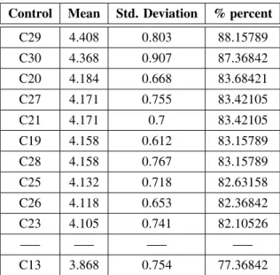
Table 4 shows the mean and the standard devi-ation for each control factor. The results of this paper show that most of the controls are used most of the time and rather often.

Control Mean Std. Deviation % percent

C29 4.408 0.803 88.15789

C30 4.368 0.907 87.36842

C20 4.184 0.668 83.68421

C27 4.171 0.755 83.42105

C21 4.171 0.7 83.42105

C19 4.158 0.612 83.15789

C28 4.158 0.767 83.15789

C25 4.132 0.718 82.63158

C26 4.118 0.653 82.36842

C23 4.105 0.741 82.10526

—– —– —– —–

C13 3.868 0.754 77.36842

Table 4.Mean score for each control factor.

5.9. Relationships Between Risks and Control Variables

Regression technique was performed on the data to determine whether there were significant re-lationships between control factors and risk fac-tors. These tests were performed using stepwise regression analysis model to compare the con-trols to each of the risk planning software de-velopment factors to determine and evaluate if they are effective in mitigating the occurrence of each risk factor. Significant relationships be-tween risks and controls, being important for the optimal models, are presented in the continua-tion. This study presents the model for software risk management within planning software de-velopment process.

R1: Risk of ‘Low Key User Involvement’ compared to controls.

Table 5, Table 6, Table 7 and Table 8 show that the obtained significant values ₍Sig.₎ are all less than the selected significant level of

C1 C2 C3 C5 C6

.336** .281* .283* .433** .524**

C10 C7 C8 C9 C11

.373** .323** .438** .460** .384**

C12 C14 C15 C19 C20

.271* .250* .264* .251* .309**

C21 C22 C24

.443** .370** .285*

*Correlation is significant at the 0.05 level(2-tailed). **Correlation is significant at the 0.01 level(2-tailed).

Table 5.Illustrates correlations between respective controls and R1.

Model R R Square Durbin-Watson

1 .524a _.275

2 .591b _.349 _1.729

a. Predictors:(constant), C6 b. Predictors:(constant), C6, C21

Table 6.Illustrates multiple correlations R, and R square.

Model _{Squares df}Sum of _SquareMean F Sig.

1 Regression 12.469 1 12.469 28.000 .000a

Residual 32.952 74 .445

Total 45.421 75

2 Regression 15.856 2 7.928 19.576 .000b

Residual 29.565 73 .405

Total 45.421 75

a. Predictors:(constant), C6 b. Predictors:(constant), C6, C21 c. Dependent variable: R1

Table 7.Illustrates an Analysis of Variance(ANOVAc₎_.

Model

Unstandardized

Coefficients StandardizedCoefficients

t Sig.

b Beta

1 (constant) 2.429 5.307 .000

C6 .476 .524 5.292 .000

2 (constant) 1.369 2.403 .019

C6 .381 .419 4.140 .000

C21 .295 .293 2.892 .005

Dependent variable: R1

Table 8.Illustrates the model coefficients, respective t values and their significance

(8)

 = 0.05, so there is a positive correlation between controls 1, 2, 3, 5, 6, 7, 8, 9, 10, 11, 12, 14, 15, 19, 20, 21, 22, 24 and Risk 1 (Table 5₎. However, the results show that Con-trols 6 and 21 have a positive impact value of

r6 = 0.524 and r21 = 0.443 respectively with

Risk 1. The multiple correlation R is 0.591, the value of R2 is 0.349 in the best model (stable model, Tables 6 and 7). This means that the Model 2 explained 34.9 % of the variability of dependent variable Risk 1. Furthermore, the Durbin-Watson statistic(D)is 1.729 and the ta-ble gives the critical values based on K ₌ 2 (regressors₎, N ₌ 76,  = 0_.05₍dU = 1.680,

dL =1.571); there is evidence of no

autocorre-lation(dU <D<2+dL: No autocorrelation).

However, we will avoid independent variables that have errors with a strong positive and nega-tive correlation in the stepwise multiple regres-sion model, because this can lead to an incorrect prediction based on independent variables.

R2: Risk of ‘Unrealistic Schedules and Budgets’ compared to controls.

Table 9, Table 10, Table 11, and Table 12 show that the obtained significant values are less than the selected significant value of  = 0.05, so there is a positive correlation between Controls 1, 3, 5, 6, 7, 8, 9, 10, 11, 24, 25, and Risk 2, respectively. In addition, Control 1 has an im-pact on Risk 2, and the results show that Con-trol 1 has a positive impact value of R=0.389 and the value of R2 _{is 0.151. This means}

that the model ₍Table 10₎ explained 15.1% of

C1 C3 C5 C6 C7 C8

.389** .297** .330** .355** .243* .229*

C9 C10 C11 C24 C25

.232* .349** .251* .331** .238*

*Correlation is significant at the 0.05 level(2-tailed). **Correlation is significant at the 0.01 level(2-tailed).

1 .389a _.151 _2.227

a. Predictors:(constant), C1

Table 10.Illustrates multiple correlation R, and R square.

1 Regression 5.817 1 5.817 13.204 .001a

Residual 32.604 74 .441

Total 38.421 75

a. Predictors:(constant), C1 b. Dependent variable: R2

Table 11. Illustrates an Analysis of Variance

(ANOVAb₎_.

Model

Unstandardized

t Sig.

b Beta

1 (constant) 2.844 5.553 .000

C1 .376 .389 3.634 .001

a. Dependent variable: R2

Table 12.Illustrates the model coefficients, respective t values and their significance(coefficientsa₎_.

the variability of response Risk 2. Further-more, Durbin-Watson statistic₍D₎is 2.227, and dU = 1.652, dL = 1.598 based on K = 1,

N = 76,  = 0.05; there is evidence of no autocorrelation(dU < D < 2+dL: No

auto-correlation).

R3: Risk of ‘Misunderstood / Unrealistic Scope and Objectives (Goals)’ compared to controls.

Table 13, Table 14, Table 15, and Table 16 show that the obtained significant values are less than the selected significant value of  = 0.05, so there is a positive correlation between Controls 1, 6, 10, 19, 30, and Risk 3, respectively. In ad-dition, Control 6 has an impact on Risk 3, and

C1 C6 C10 C19 C30

.254* .264* .247* .264* .235*

*Correlation is significant at the 0.05 level(2-tailed).

1 .264a _.070 _1.812

(9)

1 Regression 4.702 1 4.702 5.538 .021a Residual 62.825 74 .849

Total 67.526 75

Table 15.Illustrates an Analysis of Variance

(ANOVAb₎_.

Model

Unstandardized

t Sig.

b Beta

1(constant) 3.455 5.469 .000

C6 .292 .264 3.634 .021

Table 16.Illustrates the model coefficients, respective t values and their significance(coefficientsa₎_. the results show that Control 6 has a positive impact value of R=0.264 and the value of R2 is 0.070. This means that the model(Table 14) explained 7.0% of the variability of response Risk 3. Furthermore, Durbin-Watson statistic (D) is 1.812, and (dU = 1.652, dL = 1.598)

based on K = 1, N = 76,  = 0.05; there is evidence of no autocorrelation because of the rule(dU<D<2+dL: No autocorrelation). R4: Risk of ‘Insufficient / Inappropriate Staffing’ compared to controls.

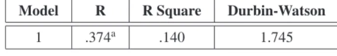
Table 17, Table 18, Table 19, and Table 20 show that the obtained significant values are less than the selected significant value of  = 0.05, so there is a positive correlation between Controls 1, 3, 5, 6, 7, 8, 9, 10, 11, 24, 28, and Risk 4, re-spectively. In addition, Control 6 has an impact on Risk 4, and the results show that Control 6 has a positive impact value ofR=0.374 and the value of R2_{is 0.140. This means that the model}

(Table 18) explained 14.0% of the

variabil-C1 C3 C5 C6 C7 C8

.285* .266* .313** .374** .247* .291*

C9 C10 C11 C24 C28

.276* .309** .249* .225* .263*

1 .374a _.140 _1.745

Table 18. Illustrates multiple correlation R, and R square.

1 Regression 9.898 1 9.898 12.031 .001a

Residual 60.879 74 .823

Total 70.776 75

(ANOVAb₎_.

Model

Unstandardized

t Sig.

b Beta

1(constant) 2.544 4.091 .000

C6 .424 .374 3.634 .001

a . Dependent variable: R4

ity of response Risk 4. Furthermore, Durbin-Watson statistic(D)is 1.745, and(dU =1.652,

dL = 1.598) based on K = 1, N = 76,

 = 0_.05; there is evidence of no autocorre-lation because of the rule₍dU < D < 2+dL:

No autocorrelation).

R5: Risk of ‘Lack of Senior Management Commitment and Technical Leadership’ compared to controls.

Table 21, Table 22, Table 23, and Table 24 show that the obtained significant values are less than the selected significant value of  = 0.05, so there is a positive correlation between Controls 1, 2, 3, 4, 5, 6, 7, 8, 9, 10, 11, 16, 18, 19, 20, 21, 22, 24, 25, 28, and Risk 5, respectively. Controls 6 and 16 have an impact on Risk 5. In addition, the results show that Controls 6, 16 have a positive impact value of 0.433, 0.329 re-spectively, multiple correlation is R=0.498 and value of R2_{is 0.248. This means that the model}

(10)

C1 C2 C3 C4 C5

.370** .272* .309** .233* .390**

C6 C7 C8 C9 C10

.433** .293* .293* .308** .307**

C11 C16 C18 C19 C20

.277* .329** .254* .256* .231*

C21 C22 C24 C25 C28

.294* .243* .232* .286* .283*

1 .433a _.187

2 .498b _.248 _2.427

Table 22. Illustrates multiple correlations R, and R square.

1 Regression 10.799 1 10.799 17.045 .000a

Residual 46.885 74 .634

Total 57.684 75

2 Regression 14.311 2 7.156 12.043 .000b

Residual 43.373 73 .594

Total 57.684 75

c. Dependent variable: R5

Table 23.Illustrates an Analysis of Variance(ANOVAc₎_.

Model

Unstandardized

t Sig.

b Beta

1(constant) 2.410 4.415 .000

C6 .443 .443 4.129 .000

2(constant) 1.077 1.414 .162

C6 .391 .382 3.683 .000

C16 .319 .252 2.431 .018

Table 24.Illustrates the model coefficients, respective t values and their significance

(coefficientsa_{, coefficients}b₎_.

based on K=2, N=76, =0.05; there is ev-idence of no autocorrelation(dU<D<2+dL:

R6: Risk of ‘Poor /Inadequate Software Project Planning and Strategic Thinking’ compared to controls.

Table 25, Table 26, Table 27, and Table 28 show that the obtained significant values are less than the selected significant value of  = 0.05, so there is a positive correlation between Controls 3, 4, 5, 6, 14, and Risk 6, respectively. Con-trols 5, 14, and 27 have an impact on Risk 6. In addition, the results show that Controls 5, 14

C3 C4 C5 C6 C14

.267* .249* .268* .228* .254**

1 .268a _.072

2 .351b _.123

3 .423c _.179 _2.006

a. Predictors:(constant), C5 b. Predictors:(constant), C5, C14 c. Predictors:(constant), C5, C14, C27

1 Regression 3.170 1 3.170 5.740 .019a

Residual 40.869 74 .552

Total 44.039 75

2 Regression 5.411 2 2.705 5.112 .008b

Residual 38.629 73 .529

Total 44.039 75

3 Regression 7.884 3 2.628 5.234 .003c

Residual 36.155 72 .502

Total 44.039 75

a. Predictors:(constant), C5 b. Predictors:(constant), C5, C14 c. Predictors:(constant), C5, C14, C27 d. Dependent variable: R6

(11)

Model

Unstandardized

t Sig.

b Beta

1(constant) 3.499 6.352 .000

C5 .256 .268 2.396 .019

2(constant) 2.394 3.145 .002

C5 .232 .243 2.201 .031

C14 .245 .227 2.058 .043

3(constant) 2.715 3.594 .001

C5 .292 .306 2.750 .008

C14 .377 .350 2.894 .005

C27 -.247 -.277 -2.219 .030

Table 28.Illustrates the model coefficients, respective t values and their significance(coefficientsa_,

coefficientsb_{, coefficients}c₎_.

have a positive impact value of 0.268 and 0.254, respectively, multiple correlation is R=0.423 and the value of R2 is 0.179. This means that the model (Table 26) explained 17.9% of the variability of response Risk 6. Also, Durbin-Watson statistic(D)is 2.006, and(dU=1.709,

dL = 1.543) based on K = 3, N = 76,  = 0.05; there is evidence of no autocorre-lation(dU <D<2+dL: No autocorrelation).

R7: Risk of ‘Lack of an Effective Software Project Management Methodology’

compared to controls.

Table 29, Table 30, Table 31, and Table 32 show that the obtained significant values are less than the selected significant value of  = 0.05, so there is a positive correlation between Controls 24, 25 and Risk 7, respectively. In addition, Control 24 has an impact on Risk 7, and the results show that Control 24 has a positive im-pact value of R₌0.394 and the value of R2 _is

0.155. This means that the model ₍Table 30₎ explained 15.5% of the variability of response Risk 7. Furthermore, Durbin-Watson statistic (D) is 1.933, and (dU = 1.652, dL = 1.598)

based on K = 1, N = 76,  = 0.05; there is evidence of no autocorrelation because of the rule₍dU<D<2+dL: No autocorrelation).

r C24 C25

R7 .394** .294*

1 .394a _.155 _1.933

Table 30. Illustrates multiple correlation R, and R square.

1 Regression 7.387 1 7.387 13.582 .000a

Residual 40.245 74 .544

Total 47.632 75

(ANOVAb₎_.

Model

Unstandardized

t Sig.

b Beta

1(constant) 2.327 3.566 .001

c24 .469 .394 3.685 .000

R8: Risk of ‘Change in Organizational Management During the Software Project’ compared to Controls.

R C17

R8 .255*

1 .255a _.065

2 .374b _.140

3 .444c _.197

4 .496d _.246 _1.883

d. Predictors:(constant), C17, C27, C25, C6

(12)

Total 57.632 75

2 Regression 8.075 2 4.037 5.947 .004b Residual 49.557 73 .679

Total 57.632 75

3 Regression 11.368 3 3.789 5.898 .001c Residual 46.263 72 .643

Total 57.632 75

4 Regression 14.198 4 3.550 5.803 .000d Residual 43.433 71 .612

Total 57.632 75

a. Predictors:(constant), C17 b. Predictors:(constant), C17, C27 c. Predictors:(constant), C17, C27, C25 d. Predictors:(constant), C17, C27, C25, C6

e. Dependent variable: R8

Table 35.Illustrates an Analysis of Variance(ANOVAe₎_.

Model

Unstandardized

t Sig.

b Beta

1(constant) 3.269 5.093 .000

C17 .282 .255 2.273 .026

2(constant) 4.268 5.802 .000

C17 .389 .352 3.060 .003

C27 -.295 -.290 -2.521 .014 3(constant) 3.457 4.320 .000

C17 .344 .311 2.741 .008

C27 -.397 -.391 -3.243 .002

C25 .306 .268 2.264 .027

4(constant) 2.723 3.196 .002

C17 .320 .290 2.608 .011

C27 -.441 -.434 -3.637 .001

C25 .287 .251 2.166 .034

C6 .236 .230 2.151 .035

coefficientsb_{, coefficients}c_{, coefficients}d₎_.

Table 33, Table 34, Table 35, and Table 36 show that the obtained significant values are less than

the selected significant value of  = 0.05, so there is a positive correlation between Control 17 and Risk 8. In addition, Controls 6, 17, 25, and 27 have an impact on Risk 8, multiple cor-relation value R=0.496, and the value of R2 is 0.246. This means that the model (Table 34) explained 24.6% of the variability of response Risk 8. Furthermore, Durbin-Watson statistic (D₎ is 1.883, and ₍dU = 1.543, dL = 1.709)

based on K=4, N=76, =0.05; there is ev-idence of no autocorrelation(dU<D<2+dL:

R9: Risk of ‘Ineffective Communication Soft-ware Project System’ compared to Controls.

Table 37, Table 38, Table 39, and Table 40 show that the obtained significant values are less than the selected significant value of  = 0.05, so there is a positive correlation between Controls 24, 27, 25, 5, and Risk 9. Controls 24, 27, 25, and 5 have an impact on the Risk 9. In addition, multiple correlation value R₌0.500, and the value of R2 _{is 0.250. This means}

that the model (Table 38) explained 25.0% of the variability of response Risk 9. Further-more, Durbin-Watson statistic(D)is 1.687, and (dU = 1.739, dL = 1.515) based on K = 4,

N ₌76,  = 0_.05; there is evidence of incon-clusive(dL <D<dU: Inconclusive).

R C24 C26

R9 .272* .233*

1 .272a _.074

2 .387b _.150

3 .448c _.201

4 .500d _.250 _1.687

d. Predictors:(constant), C24, C27, C25, C5

(13)

Total 51.789 75

2 Regression 7.772 2 3.886 6.445 .003b Residual 44.017 73 .603

Total 51.789 75

3 Regression 10.402 3 3.467 6.032 .001c Residual 41.378 72 .575

Total 51.789 75

4 Regression 12.951 4 3.238 5.919 .000d Residual 38.838 71 .547

Total 51.789 75

d. Predictors:(constant), C24, C27, C25, C5 e. Dependent variable: R9

Table 39.Illustrates an Analysis of Variance(ANOVAe₎_.

Model

Unstandardized

t Sig.

b Beta

1(constant) 3.233 4.539 .000

C24 .338 .272 2.427 .018

2(constant) 4.090 5.353 .000

C24 .461 .371 3.233 .002

C27 -.283 -.293 -2.560 .013 3(constant) 3.560 4.530 .000

C24 .360 .289 2.448 .017

C27 -.365 -.378 -3.186 .002

C25 .285 .263 2.139 .036

4(constant) 2.762 3.245 .002

C24 .275 .221 1.853 .068

C27 -.428 -.444 -3.708 .000

C25 .341 .315 2.571 .012

C5 .249 .241 2.159 .034

coefficientsb_{, coefficients}c_{, coefficients}d₎_.

R10: Risk of ‘Absence of Historical Data (Templates)’ compared to Controls.

Table 41, Table 42, Table 43, and Table 44 show that the obtained significant values are less than the selected significant value of  = 0.05, so

C1 C3 C4 C5 C6

.312** .354** .379** .349** .331**

C7 C8 C10 C29

.370** .253* .234* .256*

1 .379a _.143 _1.882

1 Regression 6.983 1 6.983 12.391 .001a

Residual 41.702 74 .564

Total 48.684 75

(ANOVAb₎_.

Model

Unstandardized

t Sig.

b Beta

1(constant) 3.023 5.690 .000

C4 .370 .379 3.520 .001

there is a positive correlation between Controls 1, 3, 4, 5, 6, 7, 8, 10, 29 and Risk 10, respec-tively. In addition, Control 4 has an impact on Risk 10, and the results show that Control 4 has a positive impact value R=0.379 and the value of R2_{is 0.143. This means that the model}

(Table 42₎ explained 14.3% of the variability of response Risk 10. Furthermore, Durbin-Watson statistic(D)is 1.882, and(dU =1.652,

dL = 1.598) based on K = 1, N = 76,

 = 0.05; there is evidence of no autocorre-lation because of the rule₍dU < D < 2+dL:

(14)

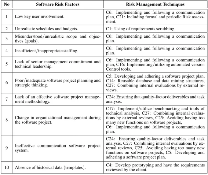
5.10. Software Risk Factors Identification Checklists and Control Factors (Risk Management Techniques)

Table 45 shows risk factors identification check-list with risk management techniques based on a questionnaire of experienced software project managers. We can use the checklist in software projects to identify and mitigate risk factors on lifecycle software projects by risk management techniques.

6. Conclusions

The concern of our paper are the modelling risks of planning software development. The results show that all risk planning software projects were very important, and important in software

project manager’s perspective, whereas all Con-trols are used most of the time, and rather often. This study incorporates risk management ap-proach and planning software development to mitigate software project failure by using step-wise multiple regression technique. These tests were performed using regression analysis( step-wise regression), in order to compare the Con-trols to each of the risk factors, to determine and evaluate if they are effective in mitigating the occurrence of each risk factor, and, finally, to select the optimal model. Only significant lationships between risks and controls were re-ported. In addition, we determined the positive correlation between risk factors and risk man-agement techniques, then measured impact risk in the software project lifecycle. We used cor-relation analysis, regression analysis, models based on the stepwise selection method(add and remove₎, and Durbin-Watson statistic.

How-No Software Risk Factors Risk Management Techniques

1 Low key user involvement. C6: Implementing and following a communicationplan, C21: Including formal and periodic Risk assess-ment.

2 Unrealistic schedules and budgets. C1: Using of requirements scrubbing.

3 Misunderstood_tives₍_goals₎_. /unrealistic scope and objec- C6: Implementing and following a communication_plan. 4 Insufficient/inappropriate staffing. C6: Implementing and following a communication_plan. 5 Lack of senior management commitment and_{technical leadership.} C6: Implementing and following a communicationplan, C16: Implementing/utilizing automated version

Control tools.

6 Poor_{strategic thinking.}/inadequate software project planning and

C5: Developing and adhering a software project plan, C14: Reusable database and data mining structures, C27: Combining internal evaluations by external re-views.

7 Lack of an effective software project manage-_{ment methodology.} C24: Ensuring that quality-factor deliverables and task_analysis.

8 Change in organizational management during_{the software project.}

C17: Implement/utilize benchmarking and tools of technical analysis, C27: Combining internal evalua-tions by external reviews, C25: Avoiding having too many new functions on software projects,

C6: Implementing and following a communication plan.

9 Ineffective communication software project_system.

C24: Ensuring quality-factor deliverables and task analysis, C27: Combining internal evaluations by ex-ternal reviews, C25: Avoiding having too many new functions on software projects, C5: Developing and adhering a software project plan.

(15)

ever, we reported the control factors in risk management approach were mitigated on risk planning software development factors in Ta-ble 45. Through the results, we found out that some controls don’t have impact, so the impor-tant controls should be considered by the soft-ware development companies in Palestinian. In addition, we cannot obtain historical data from database before using certain techniques. As future work, we intend to apply these study re-sults on a real-world software project to ver-ify the effectiveness of the new techniques and approach on a software project. We can use other techniques to manage and mitigate soft-ware project risks, such as neural network, ge-netic algorithm, Bayesian statistics, and other artificial intelligence techniques.

7. Appendix

Appendix illustrates models with an intercept (from Savin and White)

Durbin-Watson Statistic: 1 Percent Significance Points of dLand dU

and 5 Percent Significance Points of dLand dU.

K 1 2 3

N Significance dL dU dL dU dL dU

75 1% 1.448 1.501 1.422 1.529 1.395 1.557

75 5 % 1.598 1.652 1.571 1.680 1.543 1.709

K 4 5

N Significance dL dU dL dU

75 1 % 1.368 1.586 1.340 1.617

75 5 % 1.515 1.739 1.487 1.770

Acknowledgments

This study is supported by Faculty of Informa-tion and CommunicaInforma-tion Technology, Techni-cal University of Malaysia Malacca (UTeM), Malaysia and Al-Aqsa University, Palestine.

References

[1] K. SCHWALBE, Information Technology Project Management. Sixth. Course Technology, Cengage Learning, 2010, pp. 490.

[2] P. VASANT, Hybrid Mesh Adaptive Direct Search Genetic Algorithms and Line Search Approaches for Fuzzy Optimization Problems in Production Planning. In Handbook of Optimization Intelli-gent Systems Reference Library,38, I. ZELINKA, V. SNA´SELˇ , A. ABRAHAM, EDS., Berlin, Heidelberg: Springer Berlin Heidelberg, 2013, pp. 779–799.

[3] J. MILER AND J. G ´ORSKI, Supporting Team Risk Management in Software Procurement and Devel-opment Projects. In 4th National Conference on Software Engineering, 2002, pp. 1–15.

[4] C. R. PANDIAN,Applied software Risk management:

A guide for software project managers. Auerbach Publications is an imprint of the Taylor & Francis Group, 2007, pp. 246.

[5] J. HOFFER, J. GEORGE ANDJ. VALACICH, Modern

Systems Analysis and Design, 6th ed. Prentice Hall, 2011, pp. 575.

[6] J. SODHI AND P. SODHI, IT Project Management Handbook. Management Concepts, 2001, pp. 264.

[7] J. TAYLOR, Managing Information Technology Projects: Applying Project Management Strategies to Software, Hardware and Integration Initiatives. AMACOM c2004, pp. 274.

[8] B. BOEHM, Value-based software engineering.ACM

SIGSOFT Softw. Eng. Notes,28(2), pp. 1–12, Mar. 2003.

[9] A. ELZAMLY ANDB. HUSSIN, Estimating Quality-Affecting Risks in Software Projects.Int. Manag. Rev. Am. Sch. Press,7(2), pp. 66–83, 2011.

[10] K. KHANFAR, A. ELZAMLY, W. AL-AHMAD, E. EL -QAWASMEH, K. ALSAMARA, S. ABULEIL, Managing Software Project Risks with the Chi-Square Tech-nique.Int. Manag. Rev.,4(2), pp. 18–29, 2008.

[11] A. ELZAMLY, B. HUSSIN, Managing Software Project Risks with Proposed Regression Model Techniques and Effect Size Technique. Int. Rev. Comput. Softw.,6(2), pp. 250–263, 2011.

[12] A. ELZAMLY, B. HUSSIN, Managing Software Project Risks (Implementation Phase) with Pro-posed Stepwise Regression Analysis Techniques.

Int. J. Inf. Technol.,1(4), pp. 300–312, 2013.

[13] A. ELZAMLY AND B. HUSSIN, Managing Software Project Risks(Design Phase)with Proposed Fuzzy Regression Analysis Techniques with Fuzzy Con-cepts. Int. Rev. Comput. Softw., 8(11), pp. 2601– 2613, 2013.

[14] A. ELZAMLY, B. HUSSIN, Managing Software Project Risks (Planning Phase) with Proposed Fuzzy Regression Analysis Techniques with Fuzzy Concepts.Int. J. Inf. Comput. Sci.,3(2), pp. 31–40, 2014.

(16)

[16] A. ELZAMLY, B. HUSSIN, Managing Software

Project Risks(Analysis Phase)with Proposed Fuzzy Regression Analysis Modelling Techniques with Fuzzy Concepts. J. Comput. Inf. Technol., 22(2), pp. 131–144, 2014.

[17] A. ELZAMLY, B. HUSSIN, Modelling and mitigating Software Implementation Project Risks with Pro-posed Mining Technique. Inf. Eng., 3, pp. 39–48, 2014.

[18] A. ELZAMLY, Evaluation of Quantitative and Min-ing Techniques for ReducMin-ing Software Maintenance Risks. Appl. Math. Sci., 8(111), pp. 5533–5542, 2014.

[19] A. ELZAMLY, B. HUSSIN, Mitigating Software Main-tenance Project Risks with Stepwise Regression Analysis Techniques. J. Mod. Math. Front., 3(2), pp. 34–44, 2014.

[20] A. ELZAMLY, B. HUSSIN, A Comparison of Stepwise And Fuzzy Multiple Regression Analysis Tech-niques for Managing Software Project Risks: Anal-ysis Phase.J. Comput. Sci.,10(10), pp. 1725–1742, 2014.

[21] A. ELZAMLY, B. HUSSIN, A Comparison of Fuzzy and Stepwise Multiple Regression Analysis Tech-niques for Managing Software Project Risks: Im-plementation Phase. Int. Manag. Rev., 10(1), pp. 43–54, 2014.

[22] A. ELZAMLY, B. HUSSIN, An Enhancement of Framework Software Risk Management Methodol-ogy for Successful Software Development.J. Theor. Appl. Inf. Technol.,62(2), pp. 410–423, 2014.

[23] H. HOODAT, H. RASHIDI, Classification and Analy-sis of Risks in Software Engineering.Eng. Technol.,

56(32), pp. 446–452, 2009.

[24] B. BOEHM, Software Risk Management: Principles and Practices. IEEE Softw., (January), pp. 1–10, 1991.

[25] J. MILER, A Method of Software Project Risk Identification and Analysis. Gdansk University of Technology, 2005.

[26] CHAOS, The Standish Group Report. 1995.

[27] T. ADDISON, S. VALLABH, Controlling Software

Project Risks – an Empirical Study of Methods used by Experienced Project Managers. InProceedings of SAICSIT, 2002, pp. 128–140.

[28] T. ADDISON, E-commerce project development

Risks: Evidence from a Delphi survey. Int. J. Inf. Manage.,23(2003), pp. 25–40, 2003.

[29] D. ALOINI, R. DULMIN, V. MININNO, Risk

manage-ment in ERP project introduction: Review of the literature. Inf. Manag., 44(6), pp. 547–567, Sep. 2007.

[30] W. HAN, S. HUANG, An empirical analysis of Risk

components and performance on software projects. J. Syst. Softw.,80(1), pp. 42–50, Jan. 2007.

[31] S. HUANG, W. HAN, Exploring the relationship

be-tween software project duration and Risk exposure: A cluster analysis.Inf. Manag.,45(3), pp. 175–182, Apr. 2008.

[32] B. ARITUA, N. J. SMITH, D. BOWER, What Risks are common to or amplified in programmes: Evidence from UK public sector infrastructure schemes.Int. J. Proj. Manag.,29(3), pp. 303–312, Apr. 2011.

[33] R. SCHMIDT, K. LYYTINEN, M. KEIL, P. CULE, Iden-tifying Software Project Risks: An International Delphi Study.J. Manag. Inf. Syst.,17(4), pp. 5–36, 2001.

[34] M. KEIL, P. CULE, K. LYYTINEN, R. SCHMIDT, A Framework for Identifying Software Project Risks. Commun. ACM,41(11), pp. 76–83, 1998.

[35] R. NAKATSU, C. IACOVOU, A comparative study

of important Risk factors involved in offshore and domestic outsourcing of software development projects: A two-panel Delphi study.Inf. Manag.,

46(1), pp. 57–68, Jan. 2009.

[36] J. CHEN, S. HUANG, An empirical analysis of the

impact of software development problem factors on software maintainability.J. Syst. Softw.,82(6), pp. 981–992, Jun. 2009.

[37] M. KEIL, A. TIWANA, A. BUSH, Reconciling user

and project manager perceptions of IT project Risk: A Delphi study.Inf. Syst. J., 12(2), pp. 103–119, 2002.

[38] L. WALLACE, M. KEIL, A. RAI, How Software

Project Risk Affects Project Performance: An Investigation of the Dimensions of Risk and an Exploratory Model.Decis. Sci.,35(2), 2004.

[39] M. SUMNER, Risk factors in enterprise-wide/ERP

projects.J. Inf. Technol.,15(4), pp. 317–327, Dec. 2000.

[40] B. BOEHM, R. ROSS, Theory-W Software Project

Management: Principles and Examples. IEEE Trans. Softw. Eng.,15(7), pp. 902–916, 1989.

[41] KWEKU EWUSI-MENSAH, Software Development Failures: Anatomy of Abandoned Projects. The MIT Press, p. 276, 2003.

[42] G. PARE´, C. SICOTTE, M. JAANA, D. GIROUARD, Pri-oritizing Clinical Information System Project Risk Factors: A Delphi Study. In Proceedings of the 41st Hawaii International Conference on System Sciences, pp. 1–10, 2008.

[43] D. HOUSTON, G. MACKULAK, J. COLLOFELLO, Stochastic simulation of Risk factor potential ef-fects for software development Risk management. J. Syst. Softw.,59(3), pp. 247–257, Dec. 2001.

[44] B. LAWRENCE, K. WIEGERS, C. EBERT, The Top

Risks of Requirements Engineering, 2001.

[45] D. SHAFER ANDC. OFFICER, Software Risk: Why

(17)

[46] C. JONES, G. GLEN, G. ANNA, D. MILLER, Strategies

for improving systems development project success. Issues Inf. Syst.,XI(1), pp. 164–173, 2010.

[47] C. JONES, Applied Software Measurement Global Analysis of Productivity and Quality, Third. No. Third Edition. McGraw-Hill Companies, 2008, p. 662.

[48] A.-N. TAIMOUR, Why IT Projects Fail, 2005.

[49] C. MARTIN, J. PASQUIER, C. M., A. T., Software

Development Effort Estimation Using Fuzzy Logic: A Case Study. In Proceedings of the Sixth Mexi-can International Conference on Computer Science (ENC’05), pp. 113–120, 2005.

[50] X. JIN, X. XU, Remote sensing of leaf water

con-tent for winter wheat using grey relational ana-lysis (GRA), stepwise regression method (SRM)

and partial least squares (PLS). In First Interna-tional Conference on Agro-Geoinformatics (Agro-Geoinformatics), pp. 1–5, 2012.

[51] Y. LAN, S. GUO, Multiple Stepwise Regression

Analysis on Knowledge Evaluation. In Interna-tional Conference on Management of E-Commerce and E-Government, pp. 297–302, 2008.

[52] N. ZHOU, J. PIERRE, D. TRUDNOWSKI, A Stepwise Regression Method for Estimating Dominant Elec-tromechanical Modes. IEEE Trans. Power Syst.,

27(2), pp. 1051–1059, 2012.

Received:August, 2014

Revised:October, 2014

Accepted:November, 2014

Contact addresses:

Abdelrafe Elzamly Department of Computer Science Faculty of Applied Sciences Al-Aqsa University P.O.BOX: 4051 Gaza Palestine e-mail:abd elzamly@yahoo.com

Burairah Hussin Fakulti Maklumat & Komunikasi Universiti Teknikal Malaysia Melaka Locked Bag 1752, Durian Tunggal P.O.BOX: 76109 Durian Tunggal Melaka Malaysia e-mail:burairah@utem.edu.my

ABDELRAFE ELZAMLY is currently a Ph.D. student of Information and Communication Technology at the Technical University Malaysia Malaka(UTeM). Born on November 30, 1976 in Gaza, Palestine, he received his B.Sc. degree in 1999 from AI-Aqsa University, Gaza and his Master degree in Computer Information Systems in 2006 from the University of Banking and Financial Sciences. Since 1999 he has been working as a full time lecturer of Computer Science at AI-Aqsa Uni-versity. Also, from 1999 to 2007 he worked as a part time lecturer at the Islamic University in Gaza. Between 2010 and 2012 he worked as a Manager in the Mustafa Center for Studies and Scientific Research in Gaza. His research interests are in Risk management, quality software, software engineering and data mining.

(18)