arXiv:2012.09276v2 [cs.LG] 5 Jan 2021
A PREPRINT
Julian Zaidi∗ Ubisoft - La Forge
Jonathan Boilard
École de technologie supérieure
Ghyslain Gagnon
École de technologie supérieure
Marc-André Carbonneau∗ Ubisoft - La Forge
January 7, 2021
A
BSTRACTLearning to disentangle and represent factors of variation in data is an important problem in AI. While many advances are made to learn these representations, it is still unclear how to quantify dis-entanglement. Several metrics exist, however little is known on their implicit assumptions, what they truly measure and their limits. As a result, it is difficult to interpret results when comparing different representations. In this work, we survey supervised disentanglement metrics and thoroughly analyze them. We propose a new taxonomy in which all metrics fall into one of three families: intervention-based, predictor-based and information-based. We conduct extensive experiments, where we isolate representation properties to compare all metrics on many aspects. From experiment results and anal-ysis, we provide insights on relations between disentangled representation properties. Finally, we provide guidelines on how to measure disentanglement and report the results.
Keywords Representation Learning·Disentanglement·Metrics
1
Introduction
In recent years, learning disentangled representations has attracted a lot of attention from the machine learning commu-nity [1–25]. A disentangled representation independently captures true underlying factors that explain the data. Such representations offer many advantages: when used on downstream tasks, they improve predictive performance [15,16], reduce sample complexity [6, 18, 26, 27], offer interpretability [1, 26], improve fairness [17] and have been identified as a way to overcomeshortcut learningin deep learning [28].
Originally, disentanglement was evaluated by visual inspection, but recent research efforts were devoted to propose metrics for more rigorous evaluations [1–13]. Most of the time, a new metric is proposed alongside a new represen-tation learning method to highlight benefits not captured by existing metrics. Unfortunately, so far, it has often been unclear what these metrics quantify or not, and under which conditions [4, 9, 11, 16, 29]. Fair quantitative evaluation is important to assess research progress by comparing new representation learning methods with the state-of-the-art, but also equally important for practitioners when performing model selection and hyper-parameter tuning [12].
While most metrics correlate on simple data sets, they do not on more complex and realistic data [16]. Moreover, this correlation does not mean that they lead to the selection of the same model, as observed in [4, 16, 29]. We highlight this problem in our experiments in Section 5.1. Having metrics leading to different conclusions means that before choosing a model or a hyper-parameter setting, one must chose an appropriate metric for the application. This is not a
trivial task because existing metrics measure different properties of disentanglement and pose different, often implicit, assumptions on these properties. Moreover, these metrics are sometimes complex procedures themselves subject to hyper-parameter configuration. The goal of this paper is to provide some guidance to practitioners for selecting the appropriate metric for their application.
Very few papers discuss how to measure disentanglement. In [16], the authors conduct a large-scale study on disen-tanglement in the unsupervised setting. Their main conclusion is that disentangling predefined factors is impossible without inductive bias, and that random seeds and hyper-parameters have a greater impact on performance than the architecture of the studied models. They also conducted experiments to measure the degree of agreement of the six metrics used in the paper. They found that five of the six metrics correlate on the simple dSprites data set [1], but only mildly on other more realistic data sets. Unfortunately, no interpretations is given onto why one of the metrics sometimes inversely correlates with the others, or why metrics measuring different properties strongly correlate. In [5], the authors propose a framework for the evaluation of disentangled representations. They identify three desirable prop-erties of a disentangled representation: explicitness, compactness and modularity. They introduce the idea that these properties should be quantified separately. They propose a new metric decomposed in three parts. The key idea of measuring different properties separately is also advocated in [6]. The authors point out that one of the three properties, compactness, is of lesser interest in practical scenarios. We will discuss these properties in detail in Section 2. To our knowledge, [11] is the only study focusing on comparing metrics. The authors organize metrics based on the basic disentanglement properties they measure. Then, they verify that metrics assign a high score to all perfect repre-sentations and a low score to all reprerepre-sentations that do not satisfy the measured property. Through demonstrations, they expose fail cases for several metrics. This constitutes a significant step towards the theoretical analysis of metrics in extreme cases.
In this paper, we propose an in-depth analysis of supervised disentanglement metrics with real-world applications in mind. We establish a clear taxonomy of metric families and underline their strengths and shortcomings. We compare the metrics with respect to many practical considerations such as robustness to noise and hidden factors, nonlinear relationship, accuracy, calibration and computational efficiency. We conduct experiments that abstract the representation learning model and data, which allows to generate representations for which we can accurately control and isolate the properties under study. Moreover, it also alleviates difficulties related to the identification of ground truth generative factors in data sets. We focus our analysis onsupervisedmetrics (i.e. metrics that require ground truth factors) since there exist very fewunsupervisedmetrics [9, 12, 13]. To our knowledge, this is the first time that such extensive and fully controlled experiments are conducted, and that metrics are compared in depth.
Contributions:
• We carry out an extensive review of disentanglement metrics, where we expose underlying assumptions, implementation complexity and other practical considerations.
• We establish a clear taxonomy of metric families and underline their strengths and short-comings.
• We conduct experiments that evacuate ambiguities introduced by learning algorithms and data sets to directly measure a metric’s performance.
• We release our code to allow for the use of our metric implementations and the reproduction of our experi-ments2.
• We provide recommendations for meaningful comparison between representations, as well as guidance for selecting appropriate metrics depending on the application context.
The rest of the paper is organized as follows: We start by identifying desirable representation properties that we wish to quantify. In Section 3, we define desirable characteristic for a metric. In Section 4, we survey existing metrics and present our taxonomy. In section 5, we present our experiments and their results. In Section 6, we discuss the implications of our findings and provide insight on how to measure disentanglement. We identify possible extensions to the paper in the conclusion.
2
2
Properties of a Disentangled Representation
Before analyzing metrics, we discuss what constitutes a disentangled representation. While there is no unanimously accepted definition of disentanglement, most agree on two main aspects [9, 14, 18, 26, 30, 31]: First, the representation has to be distributed. This means that an input is a composition of explanatory factors and corresponds to a single point in the representation space. Like in [5] we call this point acodein the remainder of this paper. Each factor is encoded
in separate dimensions of the code. In Section 2.1, we further discuss factor independence and its implications. Second, the representation should also encode relevant information for the downstream task. Depending on the application and the representation learning algorithm, the way codes and factors relate to each other may vary significantly. We discuss Information content in Section 2.2.
2.1 Factor Independence in Representation
Factor independence means that the variation in one factor does not affect other factors, i.e. there is no causal effect between them [32]. In a disentangled representation factors are also independent in the representation space. In other words, a factor affects only a subset of the representation space, and only this factor affects this subspace. Most authors agree on the importance of this property which has different names (e.g.,disentanglement[5],modularity[6]). In this paper, we use the name convention of [6] and refer to this property asmodularity.
Some authors argue that the subset of the representation space affected by a factor should be as small as possible. Ideally, only one dimension completely describes a factor. This property is calledcompletenessin [5], but is called compactnessin [6]. In this paper we refer to this property ascompactness.
The desirability of compactness relates to the type of factors for a given application. As argued in [6], enforcing compactness may be counterproductive. A group of code dimensions provides more flexibility when describing com-plex factors [33]. For instance, if an angle is represented as a single valueθ ∈ [0,2π], there is a discontinuity in the space at2π. Alternatively, if two dimensions encode the angle (e.g. sinθ andcosθ), continuity is preserved.
Furthermore, sometimes factors are complex concepts like facial expression [19] or phonetic content [21], which are unlikely describable by a 1-dimensional space. As a second argument against enforcing strict compactness, Ridgeway and Mozer [6] explain that allowing redundancy in the learned latent space allows for different equivalent solutions, which facilitate model optimization from a practical standpoint.
All metrics assume that a set of independent factors exists in the problem. However, in practice, identifying useful and interpretable independent factors represents a challenging task [23]. Factors must be conceptually independent, but should also be statistically independent [2]. This condition is hard to satisfy in real-world data sets where certain factor realizations tend to co-occur more than others [14]. For example, in a data set of fruit images, we could be interested in two conceptually different factors: fruit type and color. However, color is statistically dependent with the fruit type. Dependent factors impact modularity score. If two factors were to share information, parts of the representation relate to both. The selection of factors is application-specific and is beyond the scope of this paper.
2.2 Information Content
To be truly useful, a representation should completely describe explanatory factors of interest. In other words, it should be possible to retrieve the complete factor realization from a point in the representation space (code). We call this propertyexplicitnesslike in [14].
Perfect explicitness entails a generalizable relation between factors and codes was learned. The nature of this relation may vary and is implicitly assumed by some metrics. A linear relation between factors and codes is the simplest, and arguably most desirable, type of relation [6]. In applications like user-specified conditioned generation, learning a monotonic relation, even if not linear, allows for intuitive navigation in the representation space.
While a monotonic relation is a desirable characteristic for continuous factors, sometimes they are best described as categorical. In that case, the learning model must partition the representation space in regions corresponding to each category. The sample distribution in this space is multi-modal. Navigating this representation space by increasing the value of a code makes little sense. Measuring disentanglement with categorical factors necessitates metrics that do not make assumptions on the nature of the factor-code relation.
In [26], the authors argue that a good representation should be invariant to other factors and noise. Unfortunately, it is not always clear which factors are pertinent for the downstream tasks. This is why it is advocated to learn as many factors as possible and discard as little information as possible [19, 26].
3
Characterization of Disentanglement Metrics
Section 2 established three main properties of disentangled representations: modularity, compactness, and explicitness. This section enumerates desirable characteristics for a disentanglement metric.
Evidently, a metric should accurately measure a disentanglement property or a subset of the properties described in Section 2. Ideally the metric should not have failure modes as identified in [2, 11]. The scoring range of the metric should be calibrated. The metric should attribute the minimum score to a completely random or fully entangled representation and a perfect score to a perfectly disentangled representation. We verify this in the experiment of Section 5.2. We provide details on how to normalize the output range for metrics that were not normalized in their original implementation in Section 4.
In addition to being calibrated, a metric score should also evolve linearly with the quality of the disentanglement properties it measures. The worst-case scenario would be a metric that acts as a step function, which offers very low score interpretability and makes the comparison between two models with the same score meaningless. Moreover, such behavior renders the metric highly unstable. We evaluate howlinearlythe metric scores change with respect to explicitness in Section 5.2, as well as to compactness and modularity in Section 5.3.
As discussed in section 2.2, every metric makes an implicit assumption on the shape of the factor-code relationship. Sometimes, the application may dictate the type of relationship expected. For instance, if a linear relation is expected, metrics which penalize non-linear relations [5, 7] are best equipped to assess the quality of a representation. However, in most situations metrics should not make any assumptions and should capture nonlinear and multimodal relations. In Section 5.5 we compare metrics on monotonic and increasingly nonlinear relations.
A metric should not be overly sensitive to hyper-parameter configuration. Low parameter sensitivity ensures stability across different configurations. A metric overly sensitive to configuration behaves unpredictably and may lead to inaccurate conclusions when comparing models. Hyper-parameters can be predictor parameters (e.g., regularization weights), discretization granularity, batch size, validation protocol, etc. The best way to mitigate hyper-parameter sensitivity is to reduce the number of parameters to set in the first place.
In real-world applications, data sets are likely to be noisy. Metrics that measure compactness or modularity should be tolerant to noise, while explicitness metrics should reflect the amount of noise in the representation. We measure robustness to noise in the experiment of Section 5.2. In the context of measuring disentanglement, explaining factors that are not targeted by the metric can also be viewed as sources of noise. In most real-world applications, there will be several factors that will not be identified and measured. We evaluate tolerance to these distracting factors in Section 5.6.
Finally, there are practical considerations when choosing a metric. Some metrics have a high computational com-plexity, while others require a large number of data points to yield meaningful results. We briefly discuss these considerations in Section 6.2.
4
Metrics
This section surveys existing supervised metrics. We propose a new taxonomy that organizes metrics into three fam-ilies. A family groups metrics based on their underlying working principle. Intervention-basedmetrics compare
codes by creating subsets of data in which one or more factors are kept constant.Predictor-basedmetrics use regres-sors or classifiers to predict factors from codes. Information-basedmetrics leverage information theory principles,
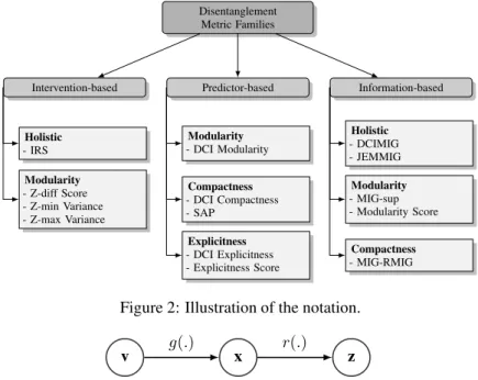
like mutual information (MI), to quantify factor-code relationships. Inspired by [11], we further divide each family in groups based on the disentanglement property that the metrics are designed to measure. Holistic methods capture two or more properties in a single score. Figure 1 shows all metrics organized following the proposed taxonomy. In the rest of this section, after introducing the notation, we go over all families in greater detail and describe metrics individually.
4.1 Notation
Inspired by [3], we denote a set ofNobservations (x) asX={x1,x2, ...,xN}. Each of these observations is assumed to be completely explained by a set ofM factorsV ={v1, v2, ..., vM}through a generative processg(v)7→ x. We denoteV = {v1,v2, ...,vN} the set of factor realizations that producedX. A representation learning algorithm is
a mappingr(x) 7→ zwherez ∈ Rd is a point in the learned code space denoted by Z = {z
1, z2, ..., zd}. Z = {z1,z2, ...,zN}is the set of all points in X projected in the code space byr(.). Supervised disentanglement metrics
Figure 1: Taxonomy of disentanglement metrics. Metrics are grouped in families based on their underlying working principle. Each family is divided in groups based on the disentanglement property that they are designed to measure.
Disentanglement Metric Families
Intervention-based Predictor-based Information-based
Holistic
- IRS
Modularity
- Z-diff Score - Z-min Variance - Z-max Variance
Modularity
- DCI Modularity
Compactness
- DCI Compactness - SAP
Explicitness
- DCI Explicitness - Explicitness Score
Holistic
- DCIMIG - JEMMIG
Modularity
- MIG-sup - Modularity Score
Compactness
- MIG-RMIG
Figure 2: Illustration of the notation.
v g(.) x r(.) z
compute a score by comparingV toZ. Figure 2 illustrates the notation. Everywhere in the paper, boldface lowercase letters represent vectors.
4.2 Intervention-based Metrics
The metrics in this family evaluate disentanglement by fixing factors and creating subsets of data points. Codes and factors in the subsets are compared to produce a score. To sample the fixed size data subsets, these methods discretize the factor space. This sampling procedure necessitates large quantities of diverse data samples to produce a meaningful score. These metrics do not make any assumptions on the factor-code relations which is their main advantage. However, there are several hyper-parameters to adjust, such as the size and the number of data subsets, the discretization granularity, classifier hyper-parameters or the choice of a distance function. Finally, failure modes, situations where the metrics wrongly score representations, were identified in [2] and [11].
4.2.1 Z-diff
Z-diff metric [1], sometimes called theβ-VAE metric, selects pairs of instances to createbatches. In a batch, a factor vi is chosen randomly. Then, a fixed number of pairs are formed with samplesv1 and
v2 that have the same value for the chosen factor (v1
i = v 2
i). Pairs are represented by the absolute difference of the codes associated with the
samples (p=
z1−z2
). The intuition is that code dimensions associated with the fixed factor should have the same value, which means a smaller difference than the other code dimensions. The mean of all pair differences in the subset creates a point in a final training set. The process is repeated several times to constitute a sizable training set. Finally, a linear classifier is trained on the data set to predict which factor was fixed. The accuracy of the classifier is the Z-diff score. For a completely random classifier we expect an accuracy of1/MwhereM is the number of factors. This can be used to scale the output closer to the[0,1]range.
4.2.2 Z-min Variance
Z-min Variance3metric [2], also called FactorVAE metric, was introduced to address some of the weaknesses of Z-diff
metric. The intuition is the same as for Z-diff: code dimensions encoding a factor should be equal, if the factor value is the same. First, all codes are normalized by their standard deviation computed over the complete data set. For as subset, a factor is randomly selected and fixed at a random value. The subset contains sampled instances for which the selected factor is fixed at the selected value. Variance is computed over the normalized codes in the subset. The code
dimension with the lowest variance is associated to the fixed factor. Several subsets are created and the factor-code associations are used as data points in a majority vote classifier. Z-min Variance score is the mean accuracy of the classifier. Like for Z-diff, random classifier accuracy of1/M can be used to scale the output closer to the[0,1]range.
4.2.3 Z-max Variance
Z-max Variance3 metric [3], also known as R-FactorVAE, is similar to Z-min Variance. The main difference is the
approach used to collect subsets of samples. Here, all factor values are fixed except one. This time, the intuition is that if all factors are the same except one, code dimensions corresponding to the free factor should exhibit higher variance. A majority vote classifier is also used to compute the score, but it is the code dimension with the highest variance that is chosen as a training point.
4.2.4 Interventional Robustness Score (IRS)
IRS [4] computes distances between sets of codes before and after an intervention on factor realizations. The intuition behind the metric is that changes innuisancefactors should not impact code dimensions attributed to targeted factors. First a reference set is created from instances where realizations of target factors are fixed. Then a second set contains instances with the same targeted factor realization, but different realizations of nuisance factors. The metric computes the distance (e.g.ℓ2) between the mean of code dimensions associated to targeted factors. This sampling and distance measurement procedure is repeated several times and the maximum observed distance is reported. The final metric reports a weighted average of the maximum distances. The distances are weighted by the frequency of the factor realizations in the data set.
4.3 Predictor-based Metrics
These metrics train regressors or classifiers to predict factor realizations from codes (f(z)7→v). Then the usefulness
of each code dimension in predicting a given factor is analyzed. These methods are naturally suited to measure explicitness. They are typically equipped to deal with continuous factors as well as categorical factors simply by choosing an appropriate predictor. However, compared to Information-based metrics, they require more design choices and hyper-parameter tuning. This means a metric is more likely to behave differently from one implementation to another.
4.3.1 Disentanglement, Completeness and Informativeness (DCI)
In [5], the authors propose a complete framework to evaluate disentangled representations instead of a single metric. They report separate scores for modularity, compactness and explicitness, which they call disentanglement, complete-ness and informativecomplete-ness. Regressors are trained to predict factors from codes. Modularity and compactcomplete-ness are estimated by inspecting the regressor’s inner parameters to infer predictive importance weightsRij for each factor and code dimension pair. In the paper, they use a linear lasso regressor or a random forest for non-linear factor-code mappings. For the lasso regressor, the importance weightsRijare the magnitudes of the weights learned by the model, while the Gini importance [34] of code dimensions is used with random forests.
The compactness for factorviis given byCi= 1 +Pd
j=1pijlogdpijwherepijis theprobabilitythat code dimension zj is important to predictvi. These probabilities are obtained by dividing each importance weight by the sum of all importance weights related to this factor:pij =Rij/Pd
k=1Rik. The compactness of the whole representation is the average compactness over all factors.
Similarly, the modularity for code dimensionzj is given byDj = 1 +PM
i=1pijlogMpijwherepijthe isprobability
that code dimensionzjis important to predict onlyvi. This time the importance weights are normalized with respect
to codes: pij = Rij/PM
k=1Rkj. The modularity score for the whole representation is a weighted average of the individual code dimension modularity scoresPd
j=1ρjDj. The scores are weighted byρjto account for codes that are less important to predict factors. The weightρjis the total importance forzjnormalized by the sum of all importance
weights:ρj =PM
i=1Rij/ Pd
k=1 PM
i=1Rik.
The prediction error of the regressor measures the explicitness of the representation. With normalized inputs and outputs, it is possible to compute the estimation error for a completely random mapping and use it to normalize the score between 0 and 1. We postulate that a representation is not explicit if the mean squared error (MSE) of the predictor is higher than the expected MSE between two uniformally distributed random variables (X andY). It can
be showed that MSE=E[(X−Y)2
] = 1/6. Thus, explicitness can be written as1−6·MSE. In our implementation, values under 0 are reported as 0.
4.3.2 Explicitness Score
In [6], the authors propose to use a classifier trained on the entire latent codes to predict factor classes, assuming that factors have discrete values. They suggest using a simple classifier such as logistic regression and report classification performance using the area under the ROC curve (ROCAUC). The final score is the average AUCROC over all classes for all factors. ROCAUC minimal value is 0.5 which means that the score needs to be normalized to obtain a value between 0 and 1. In our implementation we balance weights in the loss of the logistic regression to account for class imbalance.
4.3.3 Attribute Predictability Score (SAP)
SAP [7] attributes a scoreSijto all pairs of factorviand code dimensionzj. A linear regression predicts a continuous
factor from each code and Sij is theR2 score of the regression. For categorical factors, it fits a decision tree on codes and reports balanced classification accuracy. Scores corresponding to codes with energy below a user specified threshold (i.e.dead-codes) are set to 0. The final SAP score is obtained by computing the difference between the two highestSijfor all factors:
SAP= 1
M M X
i
Si⋆−Si◦ (1)
In this equation,Si⋆ is the highest score for factorvi, whileSi◦ is the second highest. M is the number of factors. SimilarSi⋆andSi◦means that explicitness is low if both values are low. Two similarly high values indicate that more than one code dimension encode the factor which means low compactness. This corresponds to thegapidea in MIG (Section 4.4.1)
4.4 Information-based Metrics
Information-based metrics compute a disentanglement score by estimating the mutual information (MI) between the factors and the codes. These methods require fewer hyper-parameters than intervention-based and predictor-based metrics. Moreover, they do not make assumptions on the nature of the factor-code relations.
However, while elegant in theory, in practice the estimation of entropy and MI is non-trivial. Even assessing the quality of the estimators remains an open problem [35]. It requires quantization of both spaces or a sampling procedure which needs to be parameterized. Most existing public MI-based metric implementations use the maximum likelihood estimator. For example in the widely used disentanglement_lib4MI is computed as follows:
I(v, z) =
Bv X
i=1 Bz X
j=1
P(i, j) log
P(i, j)
P(i)P(j)
(2) Factor and code spaces are discretized inBv andBzbins.P(i)andP(j)are estimated as the proportion of samples assigned to biniandjrespectively over all samples (N). SimilarlyP(i, j)is the proportion of samples assigned to both biniandj. Problems arise when estimating from under-sampled high dimensional data [36]. This is the case when computing MI, or joint entropy, between a factor and more than one dimension of the latent space. Moreover, the estimated MI value is affected by the granularity of the discretization which makes the metrics sensitive to this parameter.
4.4.1 Mutual Information Gap (MIG)
MIG [8] computes the MI between each code and factorI(vi, zj). Then, the code dimension with maximum MI is identifiedI(vi, z⋆)for each factor. After, the second highest MI,I(vi, z◦), is subtracted from this maximal value. This difference constitutes thegap. The gap is then normalized with respect to the total MI associated with the factor:
MIG=I(vi, z⋆Pd )−I(vi, z◦)
j=1I(vi, zj)
(3)
The MIG score of all factors are averaged to report one score.
Robust MIG (RMIG) was proposed in [9]. It is identical to MIG in essence, but proposes a more robust formulation when MI is computed from the input space, which does not apply in our context.
4.4.2 Joint Entropy Minus Mutual Information Gap (JEMMIG)
MIG verifies that the information related to a factor is expressed by only one code dimension (compactness). However, modularity is not directly measured. For instance a code dimension could contain information about more than one factor. JEMMIG [9] addresses this drawback by including the joint entropy of the factor and its best code.
JEMMIG=H(vi, z⋆)−I(vi, z⋆) +I(vi, z◦) (4)
As opposed to MIG, this metric indicates a high disentanglement quality with a lower score. The maximum value is bounded byH(vi) +log(Bz), whereBzis the number of bins used in the code space discretization. This means that JEMMIG can be rewritten as follows to get a score between 0 and 1:
\
JEMMIG= 1−H(vi, z⋆)−I(vi, z⋆) +I(vi, z◦)
H(vi) +log(Bz) (5)
As done for MIG, JEMMIG is reported as the average for all factorsvi.
4.4.3 MIG-sup
MIG-sup [10] is an extension of MIG. Like JEMMIG, it addresses the fact that MIG measures compactness, but does not measure modularity. It is designed to be used in conjunction with MIG. The idea is similar to MIG except that the MI gap is computed from the code point-of-view:
MIG-sup=I(zj, v⋆)−I(zj, v◦) (6)
v⋆is the factor that has the highest MI with code dimensionzj. v◦is the factor that has the second highest MI with code dimensionzj.I(zj, vi)is the MI normalized by the entropy of the factorvi. MIG-sup is reported as the average gap over all code dimensions.
4.4.4 Modularity Score
To measure modularity, in [6] the factorv⋆ which shares the maximum MI for each code dimensionzj is identified. This maximal MI valueI(v⋆, zj)is then compared with MI values of all other factors:
modularity= 1−
P
i∈V6=⋆I(i, zj) 2
I(v⋆, zj)2(M−1) (7)
We denoteV6=⋆as the set of all factors exceptv⋆andM is the number of factors. The average modularity score over
all codes is reported.
4.4.5 DCIMIG
DCIMIG [11] is a metric inspired by DCI and MIG. Like MIG, it computes MI gaps between factors and code dimensions. Like DCI it analyzes a factor-code importance matrix. However, unlike DCI, DCIMIG reports a single score for all three disentanglement properties. DCIMIG starts by computing the MI between each factor and code dimensionI(vi, zj). Then, the factor with maximum MI, I(v⋆, zj), is identified for each code. After, the second highest MI,I(v◦, zj), is subtracted from this maximal value. Thus we obtain agapfor each code dimensionRj = I(v⋆, zj)−I(v◦, zj). Each of these gapsRjrelates to a code dimension and the factor for which MI is maximal. For each factorvi, we find all associated gapsRj and use them as scoreSifor this factor. If there are more than oneRj
associated with the factor,Si equals the highestRj. If there are none,Si = 0. Finally the metric is the sum of all scores normalized by the total factor entropy:
DCIMIG=
PM i=1Si PM
i=1H(vi)
5
Experiments
In the experiments, we abstract the relation z = r(g(v))by z = f(v). Except for Section 5.1, we do not learn representations on data sets, but instead we directly definef(v)as a function that allows for complete control over the parameters of the representation evaluated by the metrics. This removes any ambiguities related to the qual-ity of the data set, the choice of learning algorithm, its training and the choice of factors to disentangle. We as-sume factors are selected followingvi |=vj, i 6=j as prescribed in [4]. The code for the experiments is available at
https://github.com/ubisoft/ubisoft-laforge-DisentanglementMetrics
5.1 Model Selection
In this experiment we verify if using different metrics to perform model selection or hyper-parameter tuning leads to different outcomes. Here, knowing the exact factor-code relation is unimportant. Therefore, we learn representations from data sets to mimic a situation a practitioner might encounter. We optimize two hyper-parameters forβ-VAE [1]: The regularization strength (β ∈ {0.001,0.01,0.1,1,10,100}) and the dimensionality of the representation space (d∈ {2,4,8,16,32,64}). We use two standard data sets Cars3D [37] and SmallNORB [38]. For each configuration, we train the model for 300k training steps using the Adam optimizer and a batch size of 64 similarly to [16]. Then, we evaluate the learned representation with every metric. For each metric, we rank the hyper-parameter configurations. We measure the agreement between all metrics using the Kendall rank correlation coefficient [39] and report results in Figure 3.
DC
I L
asso
M
od
DC
I L
asso
Co
mp
DC
I L
asso
Ex
pl
DC
I R
F M
od
DC
I R
F C
om
p
DC
I R
F E
xp
l
DC
IM
IG
Ex
pli
cit
ne
ss
Sc
ore IRS
JEM
MIG
MIG
-R
MI
G
MI
G-su
p
Mo
du
lar
ity
Sc
ore SAP Z-d
iff
Z-m
ax
Va
ria
nc
e
Z-m
in
Va
ria
nc
e
DCI Lasso Mod
DCI Lasso Comp
DCI Lasso Expl
DCI RF Mod
DCI RF Comp
DCI RF Expl
DCIMIG
Explicitness Score
IRS
JEMMIG
MIG-RMIG
MIG-sup
Modularity Score
SAP
Z-diff
Z-max Variance
Z-min Variance
100 35 -20 6 25 -7 25 -20 -3 24 22 16 12 19 -22 12 0 35 100-40 -7 22 -31 41 -37 -9 32 25 29 -19 45 24 -9 3 -20 -40100 50 34 58 -14 86 -21 -32 -20 -75 0 -11 21 40 36 6 -7 50 100 52 31 14 53 -34 -17 -6 -46 1 3 24 40 35 25 22 34 52 100 22 28 34 -39 -2 10 -43 -8 30 24 26 29 -7 -31 58 31 22 100-11 54 -23 -33 -17 -48 -7 -13 21 46 37 25 41 -14 14 28 -11100-15 -32 30 41 5 -18 9 11 -2 28 -20 -37 86 53 34 54 -15100-17 -32 -20 -72 -5 -12 22 43 37 -3 -9 -21 -34 -39 -23 -32 -17100 18 -3 36 17 -4 -17 -9 -33 24 32 -32 -17 -2 -33 30 -32 18 100 63 29 -16 -2 -20 -19 3 22 25 -20 -6 10 -17 41 -20 -3 63 100 13 -7 4 -17 -17 13 16 29 -75 -46 -43 -48 5 -72 36 29 13 100 17 7 -22 -29 -32 12 -19 0 1 -8 -7 -18 -5 17 -16 -7 17 100 4 -22 2 -22 19 45 -11 3 30 -13 9 -12 -4 -2 4 7 4 100 20 1 3 -22 24 21 24 24 21 11 22 -17 -20 -17 -22 -22 20 100 24 24 12 -9 40 40 26 46 -2 43 -9 -19 -17 -29 2 1 24 100 41 0 3 36 35 29 37 28 37 -33 3 13 -32 -22 3 24 41 100
(a) Cars3D
DC
I L
asso
M
od
DC
I L
asso
Co
mp
DC
I L
asso
Ex
pl
DC
I R
F M
od
DC
I R
F C
om
p
DC
I R
F E
xp
l
DC
IM
IG
Ex
pli
cit
ne
ss
Sc
ore IRS
JEM
MIG
MIG
-R
MI
G
MI
G-su
p
Mo
du
lar
ity
Sc
ore SAP Z-d
iff
Z-m
ax
Va
ria
nc
e
Z-m
in
Va
ria
nc
e
DCI Lasso Mod
DCI Lasso Comp
DCI Lasso Expl
DCI RF Mod
DCI RF Comp
DCI RF Expl
DCIMIG
Explicitness Score
IRS
JEMMIG
MIG-RMIG
MIG-sup
Modularity Score
SAP
Z-diff
Z-max Variance
Z-min Variance
100 44 -9 -8 19 -28 6 -23 19 19 18 20 5 20 -28 -8 -23 44 100-43 -12 22 -31 -5 -35 9 23 28 14 -16 18 -15 -7 -6 -9 -43100 33 -10 37 25 62 -14 -16 -18 -19 17 -13 7 7 4 -8 -12 33 100 47 25 40 41 -39 28 31 -36 -21 8 32 38 16 19 22 -10 47 100-21 43 -10 -10 57 63 -8 -21 21 5 32 -11 -28 -31 37 25 -21100-19 68 -58 -32 -17 -63 -28 -21 50 18 58 6 -5 25 40 43 -19100 2 14 39 37 15 12 18 -21 5 -38 -23 -35 62 41 -10 68 2 100-49 -19 -12 -55 -14 -21 43 24 43 19 9 -14 -39 -10 -58 14 -49100 3 -17 86 57 5 -73 -47 -72 19 23 -16 28 57 -32 39 -19 3 100 73 2 -14 33 -9 33 -23 18 28 -18 31 63 -17 37 -12 -17 73 100-16 -31 30 11 47 -1 20 14 -19 -36 -8 -63 15 -55 86 2 -16100 52 13 -69 -41 -70 5 -16 17 -21 -21 -28 12 -14 57 -14 -31 52 100 -4 -53 -24 -49 20 18 -13 8 21 -21 18 -21 5 33 30 13 -4 100-14 14 -18 -28 -15 7 32 5 50 -21 43 -73 -9 11 -69 -53 -14100 45 71 -8 -7 7 38 32 18 5 24 -47 33 47 -41 -24 14 45 100 30 -23 -6 4 16 -11 58 -38 43 -72 -23 -1 -70 -49 -18 71 30 100
(b) SmallNORB
Figure 3: Kendall rank correlation coefficient (×100) between metrics for model rankings.
We find that different metrics lead to different choices of models, which is consistent with results found in [4, 16, 29]. While some metrics correlate, most of the time the correlation is weak and worse, often inverse. This confirms that these metrics are not equivalent and measure different properties under different assumptions, which motivates the present study. It would be hazardous to interpret these correlations between metrics because we do not know the exact factor-code relations, which is why we devised fully parameterized relations for the subsequent experiments.
5.2 Perfect Disentangled Representation with Noise
In this section we evaluate how metrics behave in a scenario where we gradually depart from a perfect disentangled representation to a completely random representation. In a perfect representation, factors completely describe the data and have a one-to-one relation with codes. This scenario shows how metrics behave as explicitness decreases under perfect compactness and modularity. We also verify metrics are well calibrated (i.e. attribute a perfect score to perfect representation and a low score to noise). The factor-code relation is defined by:
z=f(v) = (1−α)v+αn (9) wheren ∼ U(0,1),α ∈ [0,1]andv,z ∈ RM=d. We simulate a problem with 8 factors (d = M = 8). We tried
different number of factors and found conclusions to be similar. Given a set of factor realizationsV we usef(.)to obtain its representation in the code spaceZ. The setV containsN = 20ksamples from the uniform distribution. We use the same 20k samples for all metrics. When necessary, factor values are discretized into 10 equal bins. We evaluateαat{0.0,0.2,0.4, ...,1.0}. We repeat the experiment with 100 different sampled versions ofV using 100 random seeds and report the average result. Figure 4 shows the mean score for all metrics as the noise level (α)
increases.
0.0 0.2 0.4 0.6 0.8 1.0 α
0.0 0.2 0.4 0.6 0.8 1.0
me
an
sc
ore
Intervention-based
Z-diff
Z-min Variance Z-max VarianceIRS
0.0 0.2 0.4 0.6 0.8 1.0 α
0.0 0.2 0.4 0.6 0.8 1.0
me
an
sc
ore
Predictor-based
DCI Lasso Mod DCI Lasso Comp DCI Lasso Expl
DCI RF Mod DCI RF Comp DCI RF Expl
Explicitness Score SAP
0.0 0.2 0.4 0.6 0.8 1.0 α
0.0 0.2 0.4 0.6 0.8 1.0
me
an
sc
ore
Information-based
MIG-RMIG
MIG-sup JEMMIGModularity Score DCIMIG
Figure 4: Metric scores for perfectly disentangled representations under increasing noise level (α).
Most metrics recognize a perfect representation and attribute a perfect score. There are three exceptions. IRS is unlikely to produce a perfect score for any representation because it computes a distance between codes for factors that arebinnedtogether. Factors in the same bin are likely to differ within the range of the bin, which in turn results in small distances in code values for the same factor bin. This explains why IRS cannot attribute a perfect score to a perfect representation. To circumvent this problem, smaller discretization needs to be applied if the number of samples is large enough for the given application. The Explicitness score is the average of ROCAUC forM×10 = 80logistic regression classifiers trained in a one-versus-the-rest strategy. One classifier is trained for each bin value per factor. The optimizer does not consistently find the optimal solution for all classifiers which leads to an ROCAUC under 1. Z-max Variance requires a dense combination of factor values to sample meaningful batches for the majority vote classifier. The 20k examples used in the experiment, when discretized in 10 bins, do not provide enough examples for a same factors realization. The direct consequence is a biased estimation of the variance, which causes a score under 1 for a perfect representation and a score higher than 0 for a completely random representation. To circumvent this problem, coarser discretization needs to be applied, which in turn might lead to an overestimation of the scores. The majority of metrics attribute a score near 0 to complete noise. However, DCI for modularity and compactness scores the representation over 0.3 when using a lasso regressor. Even if the regressor accuracy is low, weights are still learned and compared to compute compactness and modularity scores. The regularization term in lasso pushes some weights towards 0 and thus sizable differences between them will be observed. This leads to observing random isolated factor-code relations which drive the score up. When using the Modularity score, the MI between each factor and code dimension should be similar. However, maximal MI value normalizes the score, which leads to a wrongfully optimistic value in most experiments in this paper.
When measuring explicitness under noise, an ideal metric score should steadily decrease as the noise level increases. IRS is a perfect example of a score that decreases linearly with noise. In fact, most metrics that focus on explicitness perform adequately. If explicitness metric scores should decrease in the presence of noise, we expect a different behavior from modularity or compactness metrics. Ideally, a metric should recognize these disentanglement properties, even in noisy representations. The predictor-based DCI exhibits a high noise robustness, which makes sense since predictors naturally discard noise information to improve generalization. This being said, their tendency to observe random isolated factor-code relations discussed above inflates this perception of noise robustness. In addition to being well calibrated, intervention-based metrics Z-diff and Z-min Variance also proved to be quite robust. Inversely, this experiment exposes the vulnerability to noise of information-based metrics. Noise causes codes to be assigned to neighbouring bins which decreases the observed MI between factors and codes.
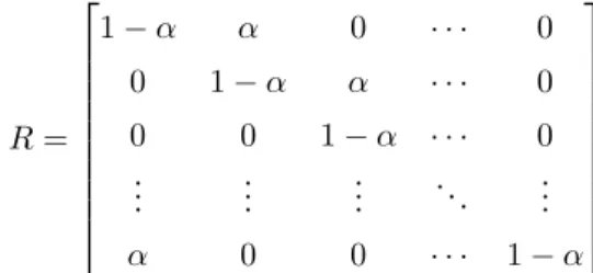
5.3 Decreasing Compactness and Modularity
In the previous section we observed how metrics behave as explicitness decreases. Now, we study what happens as we gradually decrease compactness and modularity, while explicitness remains perfect. The embedding function is constructed given byz=f(v) =vR. The projection matrixRis defined by:
R=
1−α α 0 · · · 0
0 1−α α · · · 0
0 0 1−α · · · 0
..
. ... ... . .. ...
α 0 0 · · · 1−α
Whenα= 0,Ris the identity matrix and the representation is perfectly compact and modular. Asαincreases, all factors are represented by two code dimensions and each code dimension relates to two factors. Figure 5 shows how metric scores evolve as the representation becomes less modular and less compact.
0.0 0.1 0.2 0.3 0.4 0.5 α
0.0 0.2 0.4 0.6 0.8 1.0
me
an
sc
ore
Intervention-based
Z-diff
Z-min Variance Z-max VarianceIRS
0.0 0.1 0.2 0.3 0.4 0.5 α
0.0 0.2 0.4 0.6 0.8 1.0
me
an
sc
ore
Predictor-based
DCI Lasso Mod DCI Lasso Comp DCI Lasso Expl
DCI RF Mod DCI RF Comp DCI RF Expl
Explicitness Score SAP
0.0 0.1 0.2 0.3 0.4 0.5 α
0.0 0.2 0.4 0.6 0.8 1.0
me
an
sc
ore
Information-based
MIG-RMIG
MIG-sup JEMMIGModularity Score DCIMIG
Figure 5: Mean metric scores as the representation becomes less modular and less compact.
Results from this experiment reveal several differences amongst metrics. Since the representation allows for complete recovery factor values, explicitness metrics maintain a high score as expected. We would expect modularity and compactness metric scores to linearly decrease asαincreases. This is the case for most information-based metrics and predictor-based metrics. Interestingly, some metrics output a 0 score when a code dimension relates to two factors or vice versa. This means that these metrics make no distinction between a representation where a code dimension relates to two factors and a representation where a code dimension relates to all factors. DCI is the best equipped metric to quantify this distinction because it will never yield a zero score unless all codes are equally relevant to predict the factors. The experiment also reveals a failure mode of intervention-based metrics as identified in [11]. These metrics consistently attribute a high score to the representations even when it is imperfect. The worst case is Z-diff that attributes a perfect score even whenα= 0.5. It is always trivial for the classifier to identify a factor by finding the distinct combination of two code dimensions with to lowest difference.
5.4 Modular but not Compact
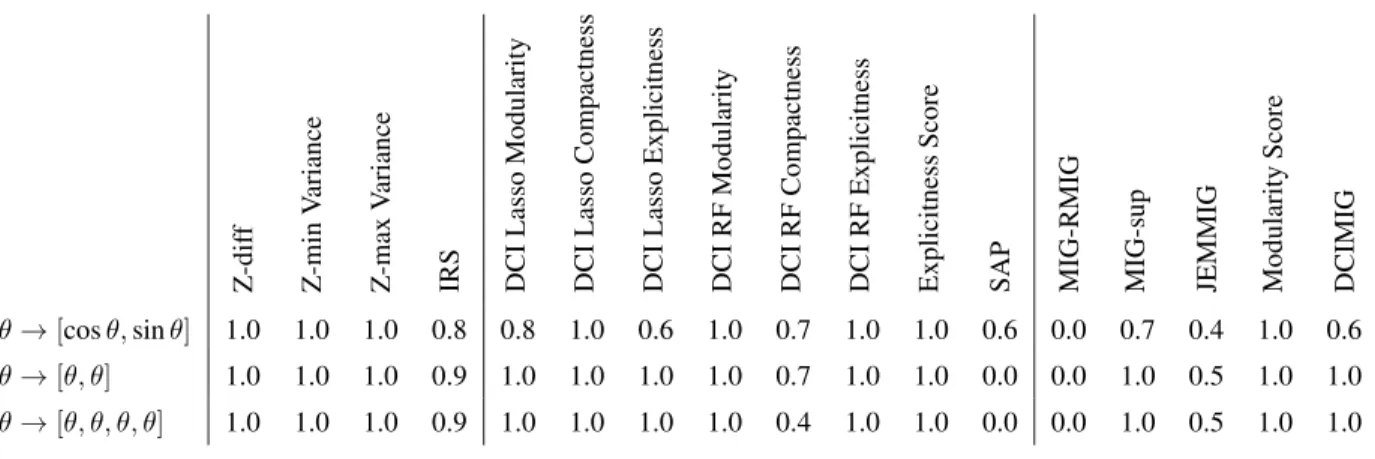
Here we evaluate how the metrics behave when the representation is perfectly explicit and modular but not compact. As discussed in Section 2.1, compactness is of lesser interest than modularity in many real-world applications. Thus, it is important to assess the ability of the metrics to recognize modularity even when several code dimensions are used to describe a single factor.
The first experiment of this section emulates a model that has learned a decomposed representation of angles. When a scalar defines an angle, the representation space has a discontinuity at2π. Decomposing angles in sine and cosine values ensures the space is continuous which is preferred in many applications. Here, each factor represents an angle
θ∈[0,2π[. Codes represent angles as cosθand sinθ. Factor realizations define four angles:v = [θ1, θ2, θ3, θ4]and the corresponding codes are given byz = [cosθ1,sinθ1,cosθ2, ...,sinθ4]. Factor values are discretized to 10 bins (vi∈ {0, π/5,2π/5, ...,9π/5}).
Table 1: Scores attributed to disentanglement where a factor is encoded with more that one code. Z -d if f Z -m in V ar ia nc e Z -m ax V ar ia nc e IR S D C I L as so M od ul ar it y D C I L as so C om pa ct ne ss D C I L as so E xp li ci tn es s D C I R F M od ul ar it y D C I R F C om pa ct ne ss D C I R F E xp li ci tn es s E xp li ci tn es s S co re S A P M IG -R M IG M IG -s up JE M M IG M od ul ar it y S co re D C IM IG
θ→[cosθ,sinθ] 1.0 1.0 1.0 0.8 0.8 1.0 0.6 1.0 0.7 1.0 1.0 0.6 0.0 0.7 0.4 1.0 0.6
θ→[θ, θ] 1.0 1.0 1.0 0.9 1.0 1.0 1.0 1.0 0.7 1.0 1.0 0.0 0.0 1.0 0.5 1.0 1.0
θ→[θ, θ, θ, θ] 1.0 1.0 1.0 0.9 1.0 1.0 1.0 1.0 0.4 1.0 1.0 0.0 0.0 1.0 0.5 1.0 1.0
Following the same idea, we create a second data set where factors are encoded by two code dimensions. However, this time, factor-code relations are linear. This corresponds to a scenario where the representation learning algorithm has learned redundant codes. This scenario allows for comparison of results obtained in the previous experiment without having to account for the nonlinear relations (sine and cosine). We keep the same four factors, but we use linear relations:v= [θ1, θ2, θ3, θ4]corresponds toz= [θ1, θ1, θ2, ..., θ4].
Finally, we repeat the same experiment except that there are only two factors associated with four code dimensions each: v= [θ1, θ2]corresponds toz= [θ1, θ1, θ1, ..., θ2]. Following the sampling methodology described in Section 5.2, we apply the metrics and report scores in Table 1.
On the left of the result table, we can see that none of the intervention-based metrics penalizes representations for not being compact. This is in accordance with the results from the previous experiment. Predictor-based metrics exhibit different behaviors depending on the type of predictor used. The lasso predictor, unsurprisingly, has trouble dealing with the nonlinear sine and cosine relations. More interestingly, it has problems dealing with redundant codes. Since only one code dimension is necessary to predict a factor, the information from the duplicated code dimensions is discarded, encouraged by the regularization term. This falsely leads the metric to think that only one code dimension is associated with the factor, hence the perfect compactness for all experiments. Using a random forest predictor overcomes this problem. As observed in the preceding experiment, SAP and MIG which measure compactness cannot express to what degree a representation is not compact. This is because they compute agapwhich subtracts the two most significant terms and ignores all of the others. The same can be said for JEMMIG. DCIMIG while intended as a holistic method does not penalize non-compactness in this experiment. Finally, we can observe that information-based metrics have trouble dealing with nonlinear relations. This will be discussed in greater detail in the next experiment.
5.5 Nonlinear relations
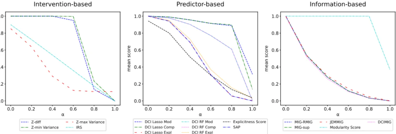
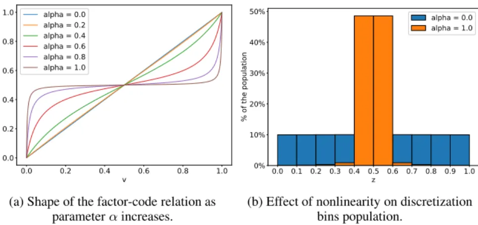
Here we explore representations with nonlinear relations between factors and codes. The representation is kept per-fectly compact and modular and should receive a perfect score from all metrics. The mapping function becomes increasingly nonlinear asαincreases, but is always monotonic forv∈[0,1]:
z=f(v) = 1000−α+0.25tan
(ω(v−0.5)) + 0.5 (10) where ω = 2arctan(1000α−0.25/2). When α= 0, the relation is practically linear, and when αis 1 the relation takes the shape of a tangent function as shown in Figure 6a. This relation is interesting because it highlights potential problems with using a linear regressor to compute scores, as well as potential problems inherent to discretization. Results are reported in Figure 7.
As expected, predictor-based metrics using a linear regression to measure explicitness, DCI lasso and SAP, under-perform as the factor-code relation becomes less linear. The monotonic nature of the relation allows DCI lasso to accurately score modularity and compactness. Naturally, a more expressive predictor makes the metric robust to more complex relationships.
This experiment highlights potential problems with discretization which is at the center of information-based metrics, as well as intervention-based metrics and even some predictor-based metrics like the Explicitness score. Equal binning of the code space results in a larger amount of the population being assigned to the middle bins. Figure 6b shows
0.0 0.2 0.4 0.6 0.8 1.0 v
0.0 0.2 0.4 0.6 0.8 1.0
z
alpha = 0.0 alpha = 0.2 alpha = 0.4 alpha = 0.6 alpha = 0.8 alpha = 1.0
(a) Shape of the factor-code relation as parameterαincreases.
0.0 0.1 0.2 0.3 0.4 0.5 0.6 0.7 0.8 0.9 1.0 z
0% 10% 20% 30% 40% 50%
%
o
f
th
e
po
pu
la
ti
on
alpha = 0.0 alpha = 1.0
(b) Effect of nonlinearity on discretization bins population.
Figure 6: Shape of the parametric factor-code relation and its effect on discretization
0.0 0.2 0.4 0.6 0.8 1.0 α
0.0 0.2 0.4 0.6 0.8 1.0
me
an
sc
ore
Intervention-based
Z-diff
Z-min Variance Z-max VarianceIRS
0.0 0.2 0.4 0.6 0.8 1.0 α
0.0 0.2 0.4 0.6 0.8 1.0
me
an
sc
ore
Predictor-based
DCI Lasso Mod DCI Lasso Comp DCI Lasso Expl
DCI RF Mod DCI RF Comp DCI RF Expl
Explicitness Score SAP
0.0 0.2 0.4 0.6 0.8 1.0 α
0.0 0.2 0.4 0.6 0.8 1.0
me
an
sc
ore
Information-based
MIG-RMIG
MIG-sup JEMMIGModularity Score DCIMIG
Figure 7: Metric scores for perfectly disentangled representations with increasingly nonlinear factor-code relation (α).
distribution lowers the code space entropy and in turn affects MI computation. Similarly, it affects how subsets are created in intervention-based metrics. This explains why a large proportion of metrics fail to properly score the perfectly modular, compact and explicit representation.
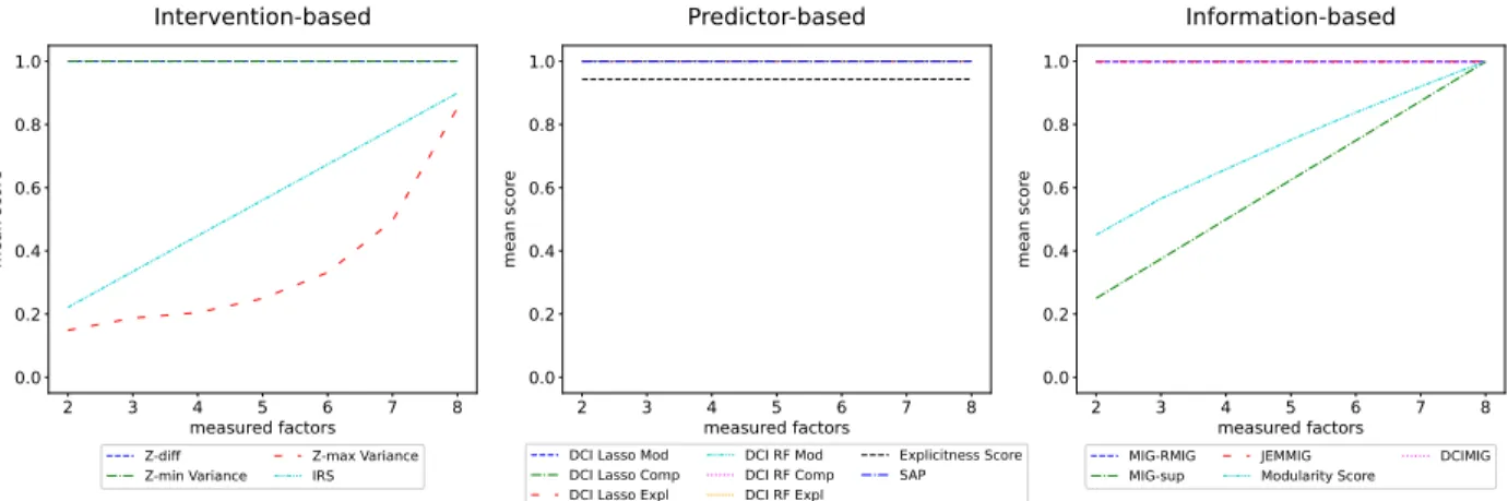
5.6 When Factors Partially Describe Data
This experiment simulates the case where metrics measure only a fraction of all the generative factors. This frequently happens in real-world scenarios because it is difficult to identify all generative factors in a data set. For instance, channel noise may corrupt data and get modeled in some dimensions of the code like in [40]. These non-measured factors still need to be encoded to preserve explicitness and because they can be useful for downstream tasks.
From the metric point-of-view, code dimensions corresponding to non-measured factors are seen as noise or dead-codes [5] which affects metric scoring. We generate perfect representations in the same way as in Section 5.2 but without noise (α= 0). The relation between factors and codes becomes the identityz=f(v) =v. Then, we apply
the metrics to these perfect representations and vary the proportion of measured factors.
When metrics measure all of the 8 generative factors captured by the perfect representation, their score should be maximal. Metrics should maintain that maximal value as the proportion of measured factors decreases because the representation does not change. Figure 8 shows how metric scores evolve as the proportion of measured factors decreases.
Most metrics are equipped to deal with non measured factors, except for Z-max Variance, IRS, MIG-sup and the Modularity score. This limits their relevance in contexts outside of academic toy problems. Successful methods that
measure disentanglement from the code point-of-view implement a mechanism to discarddead-codes[5]. A
2 3 4 5 6 7 8 measured factors
0.0 0.2 0.4 0.6 0.8 1.0
me
an
sc
ore
Intervention-based
Z-diff
Z-min Variance Z-max VarianceIRS
2 3 4 5 6 7 8 measured factors
0.0 0.2 0.4 0.6 0.8 1.0
me
an
sc
ore
Predictor-based
DCI Lasso Mod DCI Lasso Comp DCI Lasso Expl
DCI RF Mod DCI RF Comp DCI RF Expl
Explicitness Score SAP
2 3 4 5 6 7 8 measured factors
0.0 0.2 0.4 0.6 0.8 1.0
me
an
sc
ore
Information-based
MIG-RMIG
MIG-sup JEMMIGModularity Score DCIMIG
Figure 8: Scores for perfectly disentangled representations. The abscissa indicates how many of the 8 factors are measured by the metrics.
mechanisms. When sampling to create subsets, IRS and Z-max Variance implicitly assume that when all known factors are fixed, corresponding codes are also fixed. This assumption is violated when there are other sources of variation for the code than the known factors.
6
Discussion
This section summarizes our learnings from the experiment results and insights from relevant papers. After discussing relations between representation properties, we identify best practices for measuring disentanglement in real-world applications. Finally, we provide recommendations on how measurements should be reported.
6.1 Relations Between Representation Properties
While disentanglement properties can be measured separately, they are implicitly linked together. This makes the analysis of disentanglement more difficult and might have motivated the holistic approach of some metrics.
Evidently, some degree of explicitness is necessary to observe modularity or compactness otherwise it would not be relevant to compare factor-code relations. However, as shown in the experiment of Section 5.2, a high level of modularity and compactness can be observed, even when explicitness is minimal. In other words,explicitness is a necessary condition for modularity and compactness, but the magnitude of these properties does not inform on the magnitude of the explicitness.
Modularity and compactness are linked together by the size of the code space.When all factors are represented,
if the code space is the same dimensionality as the number of factors, perfect modularity necessarily implies perfect compactness. This relation is not symmetric. Perfect compactness does not necessarily means perfect modularity in this situation. A code dimension could encode two factors even if each factor is encoded by only one dimension. This would however mean that there are one or more dead-codes. As the code space increases, under perfect modularity, imperfect compactness is possible. The ratio between the code space dimensionality and the number of factors deter-mines how much compactness is allowed to deteriorate. As a general rule, the code space should be larger than the factor space to allow for composite factors and non-measured factors. The fact that the code space size links compact-ness and modularity could explain correlations sometimes observed between metrics that focus on only one of these properties like in [16].
Modularity is more important in practice than compactness. This has already been observed in [14]. There are several reasons why researchers and practitioners should focus on modularity instead of compactness. The main reason is that measuring compactness is desirable only if one can identifyatomic(1D) factors, which is often difficult or impossible in real-world applications. As mentioned earlier, some basic concepts like angle or color are best represented in a 2D or 3D space. In addition, any composite factors (e.g., object type in images or speaker identity in speech segments) are more meaningfully represented in a multi-dimensional space, where each dimension represents an atomic factor. These atomic factors are sometimes concepts difficult to identify, describe and measure. For example, if one wants to disentangle speaker identity from speech segments. Many atomic factors define a voice print. Some are simpler to identify and measure like pitch and speech rate, but they do not paint the whole picture. The complete
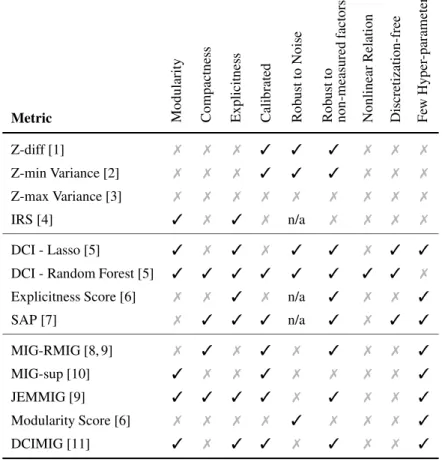
Table 2: Summary of findings from experiments and analysis. For a metric to possess a desired characteristic (✓), it
has to be true in theory, as well as in practice. The robustness to noise characteristic does not apply to explicitness metrics.
Metric Mod
ul
ar
it
y
C
om
pa
ct
ne
ss
E
xp
li
ci
tn
es
s
C
al
ib
ra
te
d
R
ob
us
tt
o
N
oi
se
R
ob
us
tt
o
no
n-m
ea
su
re
d
fa
ct
or
s
N
on
li
ne
ar
R
el
at
io
n
D
is
cr
et
iz
at
io
n-fr
ee
F
ew
H
yp
er
-p
ar
am
et
er
s
Z-diff [1] ✗ ✗ ✗ ✓ ✓ ✓ ✗ ✗ ✗
Z-min Variance [2] ✗ ✗ ✗ ✓ ✓ ✓ ✗ ✗ ✗
Z-max Variance [3] ✗ ✗ ✗ ✗ ✗ ✗ ✗ ✗ ✗
IRS [4] ✓ ✗ ✓ ✗ n/a ✗ ✗ ✗ ✗
DCI - Lasso [5] ✓ ✗ ✓ ✗ ✓ ✓ ✗ ✓ ✓
DCI - Random Forest [5] ✓ ✓ ✓ ✓ ✓ ✓ ✓ ✓ ✗
Explicitness Score [6] ✗ ✗ ✓ ✗ n/a ✓ ✗ ✗ ✓
SAP [7] ✗ ✓ ✓ ✓ n/a ✓ ✗ ✓ ✓
MIG-RMIG [8, 9] ✗ ✓ ✗ ✓ ✗ ✓ ✗ ✗ ✓
MIG-sup [10] ✓ ✗ ✗ ✓ ✗ ✗ ✗ ✗ ✓
JEMMIG [9] ✓ ✓ ✓ ✓ ✗ ✓ ✗ ✗ ✓
Modularity Score [6] ✗ ✗ ✗ ✗ ✓ ✗ ✗ ✗ ✓
DCIMIG [11] ✓ ✗ ✓ ✓ ✗ ✓ ✗ ✗ ✓
set of atomic factors for voice print remains elusive, even for speech experts. Nonetheless, they must be encoded to successfully perform a downstream task like speaker identification or conditioned speech synthesis. the same goes for illumination in a picture. In practice, one might want to isolate the effect of a light source. However, light sources have many attributes like, 3D position, color, shape, size, intensity, etc. All these factors have to be identified and quantified to measure compactness. For both these example applications, useful disentanglement is best measured through modularity. A high modularity score indicates that all atomic factors of interest are contained in a defined subset of the code space.
The factor space and the code space need to be aligned to accurately measure disentanglement. Perfect com-pactness and modularity entails complete disentanglement of generative factors. However, it is possible to learn a representation where factors are completely disentangled, and yet measure low compactness and modularity scores because of a misalignment between space axes. As a thought experiment, if we take a perfectly disentangled repre-sentation, where each factor corresponds to only one code, and rotate this representation space around any axis. The resulting rotated representation space maintains the independence between factors. However existing metrics will fail to capture perfect modularity or compactness because variations in one factor will cause variations on several dimen-sions of the code space andvice versa. We believe a metric should be robust to this kind of misalignment and be able to evaluate representations by looking at them from the right "point-of-view". In practice, axis alignment can be enforced during learning through supervision, or indirectly encouraged like in VAEs [22,41], but cannot be guaranteed in most unsupervised learning settings [16].
6.2 Practical Considerations for Choosing a Metric
In this section, we extract conclusions from our analysis and experimental results summarized in Table 2. We provide guidance for choosing an appropriate metric for real-world application, and we highlight practical considerations when measuring disentanglement.
Metrics that do not account for non-measured factors should be avoided in real-world scenarios. As discussed in Section 2.1, in practice, identifying factors is a challenging task. Identifying all factors is even more difficult. Moreover, when identified, factors must be measured which is sometimes impossible. This means that for most applications, there will exist unidentified factors explaining the data, which will cause some metrics to underestimate modularity as shown in Section 5.6.
Using discretization is not trivial and has an impact on score. As we saw in Section 5.5, discretization of the code and the factor space has considerable impact on the ability of metrics to deal with nonlinear relations. The granularity of the discretization has an impact on the estimated MI, which is the centerpiece of information-based metrics. Intuitively, MI informs on how easy it is to predict a variableAknowingB. SupposeAis a random variable andB =A+σwhereσis random noise. On one extreme, if both variables are discretized in 1 bin, then the MI is maximum. On the other end of the spectrum,AandBare discretized in a large number of narrow bins. If the number of samples is limited, it is unlikely thatBwill help predict the exact bin ofA. In that case, MI will appear to be low even if there exists a strong relation betweenAandB. In intervention-based metrics, the discretization granularity determines the degree of similarity/dissimilarity of examples grouped in the same subset. A too coarse discretization creates heterogeneous groups that are considered homogeneous, which biases results. A too fine discretization makes it impossible to create large enough subsets of data points with the same fixed value. To our knowledge, no procedure has been proposed yet to strike the right balance between coarse and fine discretization for any type of metric. Table 2 compiles our experimentation results and analysis. For a metric to possess a characteristic (✓), it has to be
true by design and not disproven experimentally. For instance, DCI with lasso regressor is marked with (✗) because it has a failure mode when measuring compactness as shown in Section 5.4, even if in theory it can measure the property. Same goes for metrics necessitating discretization when dealing with nonlinear relations.
DCI implemented with random forest is the best all around metric. Measuring disentanglement properties
sepa-rately allows for accurate scoring. Because random forest is an expressive model, it can discover nonlinear relation-ships and does not suffer from problems related to discretization. Moreover, random forests can be used as classifiers and regressors which makes them appropriate for applications mixing continuous and categorical factors. DCI imple-ments a weighting scheme that accounts for dead-codes in problems where not all factors can be identified. However, there are two important disadvantages to DCI. First, modeling relations with random forests requires a bit of expertise to set the hyper-parameters and determine a relevant criterion for code dimension importance.The hyper-parameters must be tuned using an appropriate cross-validation procedure, to ensure proper regularization of the model.
Otherwise it will overfit, which results in an overestimation of explicitness as well as an underestimation of modularity and compactness. This cross-validation procedure is time consuming which is the second main disadvantage of the method. In fact, DCI with random forest is the most computationally expensive of all metrics studied in this paper. In their current state, metrics in the intervention-based family should be used with great caution. They require large quantities of data to create subsets with fixed values. This prohibits their application in problems with limited quantities of data with labeled factors. They are subject to vulnerabilities associated with discretization. Moreover, they are prone to failure modes, which limits their reliability. Finally, unlike most metrics from other families, they do not produce a factor-code relation matrix, which makes their results difficult to interpret and less helpful when debugging.
Information-based metrics are in theory flexible and elegant. They can measure factor-code relations of any shape, continuous or categorical, with a minimal amount of hyper-parameter tuning. However, the aforementioned challenges with discretization limit their universality and makes them vulnerable to noise. Also metrics based on informationgaps like MIG, only consider the difference between the two best candidates. This limits their expressiveness. For instance in the experiment of Section 5.4, MIG attributes the same compactness score (0.0) to representations where a factor corresponds to two and four code dimensions. We believe that if these limitations were addressed, information-based metrics would be more interesting solutions.
6.3 Reporting Results
Disentanglement properties should be measured separately.We share this opinion with [5] and [6]. In our experi-ments, we showed we could vary properties independently and get the same overall score in very different situations. Metrics measuring all at once make the analysis and comparison of algorithms imprecise. This is particularly true in cases where a parameter balances reconstruction error and factor separation (e.g.β−VAE [1]). Using a single metric to measure both explicitness and modularity makes it impossible to determine the contribution of each property to the score.
Disentanglement should be measured for each factor independently.While global scores give a quick impression
on disentanglement quality, they do not paint the whole picture and can be deceiving. It is impossible to tell from a single number if a model performs generally well except on a few problematic factors, or equally badly on all of them.
The first case might indicate a problem with the data or the choice of factors, while in the second it indicates poor performance of the representation model.
Metrics should be run several times on the same representation. One should report average scores alongside standard deviation. Many metrics implement stochastic components. For instance, intervention-based metrics
sam-ple subsets on which they rest their analysis. Predictor-based metrics create validation sets to perform hyper-parameter tuning. Moreover, in applications with large data sets, representations are evaluated on a subset of samples for effi-ciency. This sampling process adds to the stochasticity of the evaluation even for stable metrics. Performing several measurement runs allows performing statistical significance tests on results to ascertain conclusions from experiments, which should be standard practice when comparing different solutions.
7
Conclusion
In this work we studied how to quantify disentanglement in representations. We conducted an extensive review of supervised disentanglement metrics. We analyzed and compared them experimentally with real-world applications in mind. We reviewed definitions of disentanglement and proposed a new taxonomy organizing the metrics into three families: intervention-based, predictor-based and information-based.
We highlighted the lack of correlation between the different metric scores, and exposed their differences in a series of fully controlled experiments on the robustness to noise, modularity, compactness, hidden factors, calibration and nonlinear relationships. Our experiments revealed different limitations for each metric. We showed how discretization hinders reliability under limited amount of data, noise and nonlinear factor-code relations. We found that predictor-based metrics, when parameterized with caution, were the best performing family of solutions. We discussed the importance of modularity over compactness for practical applications. We concluded, perhaps unsurprisingly, that each disentanglement property should be measured separately for better interpretability.
While we shed some light on the inner working assumption of supervised metrics, several open questions remain. We think that some of the limits exposed in the study can be solved, and thus some metrics, notably from the information-based family, could prove to be stronger solutions than they are now. Also, supervised metrics necessitate factors to be identified and measured which is not always possible when dealing with real-world data. This is why research efforts are now increasingly focused on measuring disentanglement without ground truth factors. This study intentionally left out unsupervised metrics, which is open for future work.
References
[1] I. Higgins, L. Matthey, A. Pal, C. Burgess, X. Glorot, M. Botvinick, S. Mohamed, and A. Lerchner, “β-VAE: Learning basic visual concepts with a constrained variational framework,” inInternational Conference on Learn-ing Representations, 2017.
[2] H. Kim and A. Mnih, “Disentangling by factorising,” inInternational Conference on Machine Learning, 2018. [3] M. Kim, Y. Wang, P. Sahu, and V. Pavlovic, “Relevance Factor VAE: Learning and identifying disentangled
factors,”arXiv:1902.01568, 2019.
[4] R. Suter, D. Miladinovic, B. Schölkopf, and S. Bauer, “Robustly disentangled causal mechanisms: Validating deep representations for interventional robustness,” inInternational Conference on Machine Learning, 2019. [5] C. Eastwood and C. K. I. Williams, “A framework for the quantitative evaluation of disentangled representations,”
inInternational Conference on Learning Representations, 2018.
[6] K. Ridgeway and M. C. Mozer, “Learning deep disentangled embeddings with the f-statistic loss,” inAdvances in Neural Information Processing Systems, 2018.
[7] A. Kumar, P. Sattigeri, and A. Balakrishnan, “Variational inference of disentangled latent concepts from unla-beled observations,” inInternational Conference on Learning Representations, 2018.
[8] R. T. Q. Chen, X. Li, R. B. Grosse, and D. K. Duvenaud, “Isolating sources of disentanglement in variational autoencoders,” inAdvances in Neural Information Processing Systems, 2018.
[9] K. Do and T. Tran, “Theory and evaluation metrics for learning disentangled representations,” inInternational Conference on Learning Representations, 2020.
[10] Z. Li, J. V. Murkute, P. K. Gyawali, and L. Wang, “Progressive learning and disentanglement of hierarchical representations,” inInternational Conference on Learning Representations, 2020.