Real time haptic and visual simulation of bone dissection

Real–time haptic and visual simulation of bone dissection

Antonio Zorcolo CRS4

VI Strada Ovest, Z. I. Macchiareddu, I-09010 Uta (CA), Italy {magus,giach,gobbetti,zag,zarco}@crs4.it – http://www.crs4.it

October 4, 2002

Abstract

Bone dissection is an important component of many surgical procedures. In this paper, we discuss a haptic and visual simulation of a bone cutting burr, that it is being devel-oped as a component of a training system for temporal bone surgery. We use a physically motivated model to describe the burr–bone interaction, that includes haptic forces eval-uation, the bone erosion process and the re-sulting debris. The current implementation, directly operating on a voxel discretization of patient-specific 3D CT and MR imaging data, is efficient enough to provide real–time feed-back on a low–end multi–processing PC plat-form.

1

Introduction

Bone dissection is an important component of many surgical procedures. In this paper, we discuss a real–time haptic and visual imple-mentation of a bone cutting burr, that it is being developed as a component of a training simulator for temporal bone surgery. The spe-cific target of the simulator is mastoidectomy, a very common operative procedure that con-sists in the removal, by use of the burring tool, of the mastoid portion of the temporal bone. The importance of computerized tools to support surgical training for this kind of

intervention has been recognized by a num-ber of groups, which are currently developing virtual reality simulators for temporal bone surgery (e.g. [26, 22]). Our work is character-ized by the use of patient-specific volumetric object models directly derived from 3D CT and MRI images, and by a design that pro-vides realistic visual and haptic feedback, in-cluding secondary effects, such as the obscur-ing of the operational site due to the accu-mulation of bone dust and other burring de-bris. The need to provide real–time feedback to users, while simulating burring and related secondary effects, imposes stringent perfor-mance constraints. Our solution is based on a volumetric representation of the scene, and it harnesses the locality of the physical system evolution to model the system as a collection of loosely coupled components running in par-allel on a multi-processor PC platform. Pre-vious work has demonstrated the effectiveness of voxel–based representations for the genera-tion of force feedback in the case of rigid body environments (e.g., [21]), virtual clay models (e.g., [7, 13, 25, 15]), or deformable bodies (e.g., [9, 14, 12, 16]).

This article, an extended version of our IEEE Virtual Reality 2002 contribution ([6]), focuses on the modeling of the haptic and vi-sual effects of bone burring. We refer the reader to [5] for details on the other system components.

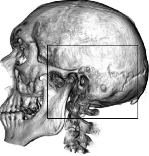
(a) The Visible Human skull (b) The mastoid region

Figure 1: Surgical site. Mastoidectomy is performed in the region indicated by the rectangle in Fig. (a) and zoomed in Fig. (b). The images are taken directly from the volumetric renderer used in the simulator. The volumetric dataset has a resolution of 256x256x219 voxels and is derived from The Visible Human Male CT Dataset made available by The National Library of Medicine.

In our model, the burr bit is represented by a region of space that samples the volu-metric bone data to construct the elastic re-action and friction forces that the bone op-poses to the burring. The sampling algorithm is similar in spirit to the Voxmap PointShell approach [21], even though here we use a vol-umetric region around the burr to select the bone voxels relevant to force calculation. Our algorithm for computing forces, loosely pat-terned on Hertz contact theory [18], is robust and a smooth function of the burr position. The computed forces are transfered to the haptic device via asample–estimate–hold [11] interface to stabilize the system. Bone ero-sion is modeled by postulating an energy bal-ance between the mechanical work performed by the burr motor and the energy needed to cut the bone, that it is assumed to be propor-tional to the bone mass removed. The actual

bone erosion is implemented by decreasing the density of the voxels that are in contact with the burr in a manner that is consistent with the predicted local mass flows. The process of accumulation of bone dust and other bur-ring debris are then handled using a particle system simulation based on simple, localized, sand-pile models. The resulting bone dissec-tion simulator provides haptic and visual ren-derings that are considered sufficient for train-ing purposes.

The rest of the paper is structured as fol-lows. Section 2 provides a brief description of the application area, while the following sec-tion is dedicated to the bone–burr interacsec-tion model. Section 4 describes how bone dust, debris, and water are simulated. Section 5 is devoted to the techniques used to provide real–time visual rendering in parallel to the simulation. Section 6 outlines how rendering

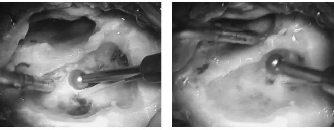
(a) Mud formation (b) Obscuring effects

Figure 2: Operation scene. These two images are typical examples of what is seen by the surgeon while performing a mastoidectomy. In (a) it is clearly visible the paste created by the mixing of bone dust with water. If the paste and the water are not removed, they can obscure the field of view (b). Photos courtesy of Prof. Stefano Sellari Franceschini, ENT Surgery, Dept. of Neuroscience, University of Pisa.

and simulation are integrated in the training system. Implementation details and results are reported in section 7. Finally the last sec-tion reports on conclusions and future work.

2

Application

area:

mas-toidectomy

Mastoidectomy consists of removal of the air cavities just under the skin behind the ear (see figure 1). It is the most superficial and com-mon surgery of the temporal bone, and it is performed for chronic infection of the mastoid air cells (mastoiditis). The mastoid air cells are widely variant in their anatomy and the main risks of the procedure are related to the detection and avoidance of the facial nerve, venous sinuses and ”dura mater”.

In the typical mastoidectomy surgical setup, the surgeon looks at the region effected by the procedure via a stereoscopic micro-scope and holds in her hands a high speed burr and a sucker, that she uses, respectively,

to cut the bone and to remove water (used to cool the burr bit) and bone paste produced by the mixing of bone dust with water, see fig. 2(a). Subjective analysis of video records, together with in-situ observations, [4], high-lighted a correlation between burring behav-iors and type and depth of bone. In the case of initial cortex burring, burr tip motions of around 0.8 cm together with sweeps over 2-4 cm were evident. Shorter (1–2 cm) mo-tions with rapid lateral strokes characterized the post-cortex mastoidectomy. For deeper burring, 1 cm strokes down to 1 mm were ev-ident with more of a polishing motion qual-ity, guided using the contours from prior bur-ring procedures. The typical sweeping move-ment speed is of about 1 mm/s. Static burr handling was also noted, eroding bone tissue whilst maintaining minimal surface pressure. The procedure requires bi-manual input, with high-quality force feedback for the dom-inant hand (controlling the burr/irrigator), and only collision detection for the non-dominant one (controlling the sucker).

Vi-sual feedback requires a microscope-like de-vice with at least 4 DOFs.

The capability of replicating the effects caused by the intertwining of the different physical processes is of primary importance for training [17, 4]. Although the presence of the water/bone paste mixture is essentially irrelevant with respect to the interaction be-tween the burr and the bone, its presence cannot be neglected in the creation of the vi-sual feed–back, because its “obscuring” effects constitute the principal cue to the user for the use of the suction device (see figure 2).

3

Bone–burr

interaction

model

A detailed mechanical description of a rotat-ing burr cuttrotat-ing bone is complicated because it involves tracking the continuously chang-ing free surface of the material bechang-ing cut; the impact of the burr blades on the surface; the resulting stress distribution in the material; and the consequent plastic deformation and break–up.

To circumvent these complications, we have divided the cutting process into two successive steps. The first estimates the bone material deformation and the resulting elastic forces, given the relative position of the burr with re-spect to the bone. For efficiency reasons, we currently do not simulate in this first step the high frequencies due to the high speed con-tact between burr bit blades and bone. This is, in our opinion, a minor limitation of the model, since human tactile sensing is limited, except for very fine feature recognition tasks, to 400Hz bandwidth [23]. The second esti-mates the local rate of cutting of the bone by using an energy balance between the mechan-ical work performed by the burr motor and the energy needed to cut the bone, that it is assumed to be proportional to the bone mass removed.

We will first describe this approach on a continuum model and then specialize the

re-sults to a discretized voxel grid. 3.1 Continuum description

3.1.1 Forces evaluation

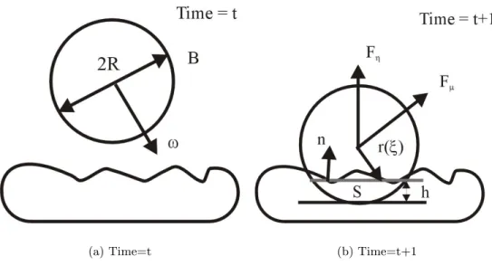
Figure 3 illustrates an idealized version of the impact of burr on bone. The burr has a spher-ical bit, of radiusR, that is rotating with an-gular velocity ~ω. At time step t the burr is just outside the bone material, while at the next time step it is intersecting the bone sur-face. In the following, we will refer to the sphere representing the burr bit asB, and to the “contact surface” between the burr and the bone as S.

All the relevant geometrical information is contained in the volumetric distribution of the bone material. We use a characteristic func-tion χ(~r) to indicate the presence/absence of bone, where~r is measured from the center of

B. The first two moments ofχ, restricted to the region contained inB are, respectively,

M =

Z

r<R

dr3χ(~r), (1)

~

M1 =

Z

r<R

dr3χ(~r)~r. (2) We can now estimate the normal direction,

ˆ

n, to S, as nˆ = −M1/~ |M1| and the “thick-ness”hofB immersed in the bone, by solving

M =πh2_(R−h

3). We can now derive,

assum-ing that _Rh << 1, and using Hertz’s contact theory [18], an expression for the total force,

~

Fe, exerted on the burr by the elastic

defor-mation of the bone:

~

Fe =C1R2( h R)

3

2ˆn, (3)

where C1 is a dimensional constant, that de-scribes the elastic properties of the material. Moreover, we can give an expression for the pressure, P~(~ξ), exerted by the burr on the pointξ~ofS:

~

P(~ξ) =− 3 2πa2

s

1−|~ξ|2

(a) Time=t (b) Time=t+1

Figure 3: The impact of burr on bone. Here we represent two successive instants, at timet

and t+ 1, of an idealized version of a surgeon burr. The burr has a spherical bit, of radius

R, that is rotating with angular velocity ~ω. The surface S is the effective “contact surface” between the burr and the bone.

whereξ~is measured from the center ofS, see fig. 3(b), and a is the radius of the contact region. In Hertz’s contact theory, a can be estimated as

a= (C1R)

1 3F

1 3

e . (5)

From equation 4, we can estimate the fric-tional force,F~µ, that the bone will oppose to

the burr rotation:

~ Fµ=µ

Z

ξ<a

dσP(~ξ)~r(

~ ξ)×~ω

|~r(~ξ)||~ω|, (6) whereµis a friction coefficient, that links the frictional forces for unit area to the locally exerted pressure.

The total force that should be returned by the haptic feedback device is, therefore,F~T =

~ Fe+F~µ.

3.1.2 Erosion modeling

We assume that all the power spent by work-ing against frictional forces goes toward the erosion of the bone material. In other words,

we equate for each “contact surface” element

dσ

µP(~ξ)ωr(ξ~) 1−(~r(~ξ)·~ω |~r(ξ~)||~ω|)

2

!

dσ=αφ(ξ~)dσ,

(7) where α is a dimensional constant and φ(~ξ) is the mass flux at the contact surface point

~

ξ. Using the mass flux φone can update the position of the bone surface.

The formulas above have been written with the implicit assumption that the burr blades are very small with respect to the burr bit radius, and that their effect can be absorbed in the friction constantµand in the “erosion constant”α. Even though this is, in general, false, and Hertz’s theory is, strictly speak-ing, only valid for small elastic deformations, this formulation provides a computationally tractable, robust, expression for the response forces that, at least in the limit of smallh, is physically reasonable.

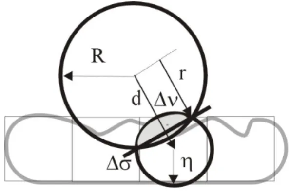
Figure 4: Voxel approximation. In order to simplify computations, voxels are approx-imated with spheres of the same volume. In this way, simple formulas for volume and sur-face intersection can be derived.

3.2 Discretized description

3.2.1 Forces evaluation

In the simulator, the bone distribution is only known at the level of a volumetric grid dis-cretized in cubic voxels. Eqs. (1,2,6) need, therefore, to be translated and re–interpreted. A direct translation will transform integrals in sums over the voxels that have non–null intersection with B. The evaluation of each voxel contribution is computationally com-plex, since it requires finding the intersections between B and the cube defining the voxel. To simplify matters, we are approximating the voxels with spheres of the same volume, centered at the voxel center, ~ci, with the

ori-gin at the center ofB. The radius of the voxel spheres,η, is, therefore, defined by 4₃πη3 =`3, where `is the length of the voxel side.

Using this approximation, it is trivial to de-rive simple formulas that express, in terms of the distance d=|~ci|, the volume, ∆V, of the

intersection region; the area, ∆σ, of the “in-tersection surface” and the actual distance,r, from the center of the intersection surface to the center of B( see fig. 4).

∆v(d) = π 12(d

3_−6(R2_+η2_)d

+ 8(R3+η3) −3(η2−R2)21

d)

(8)

∆σ(d) = π 4(2(η

2_+R2_)−d2

−(η2−R2)2 1

d2)

(9)

r(d) = 1 2d+

R2_−η2

2 1

d (10)

The required integrals then become

M∗ =X

i

∆V(|c~i|)χi (11)

and

~

M₁∗ =X

i

∆V(|c~i|)χi

ri

di

~

c1. (12)

To estimate the friction force, F~µ we

con-vert the area integral (6) in

~ Fµ=µ

X

i

∆σ(|~ci|)P(ξ~i)

~ ci×~ω

|~ci||~ω|

, (13)

with

~ ξi =

ri

di

(~ci−

(~ω·~ci)

ω2 ~ω). (14)

The power spent by the frictional forces on a voxel is then

µP(ξi)ωri(ξ~i)

1−( c~i·~ω |c~i||~ω|

)2

∆σi=αφi∆σi,

(15) whereφiis the mass flux per unit surface

com-ing out of voxeli, via surface ∆σi. To

evalu-ateP we use formula (4), where for awe use the “effective” radius of the contact surface

a∗ =√2Rh−h2_.

3.2.2 Erosion modeling

Using the fluxesφi we can now erode the

vox-els in the intersection region. In our current implementation, we associate a 8 bit counter

with each voxel, representing the voxel den-sity, and decrease it by a value proportional to the “assumed” amount of removed mass, ∆Mi = ∆t∆σφi, where ∆tis the time step of

the simulation, and the mass, Mi, contained

in the voxeli. The bone material in the tem-poral bone area has a morphological structure that ranges from compact bone, e.g., close to the outer skull surface, to a porous, “trabec-ular”, consistency. The porous scale ranges from few millimeters down to scales well be-yond the resolution of the medical imaging devices. In our model, the subscale modeling of the trabecular structures is absorbed in a voxel dependent erosion constantα.

3.3 Sample–Estimate-Hold Inter-face

A direct transmission of the computed forces to the haptic device is, in the case of “almost rigid” contacts, usually plagued by mechani-cal instabilities. The typimechani-cal solution for this problem is the introduction of an artificial, “virtual”, coupling between the haptic device and the virtual environment [8, 2].

In our system, we use a sample–estimate– hold approach [11] to remove the excess en-ergy injected by the standard zero–order hold of force employed by the haptic device drivers. With this technique, we compute the force that is sent to the haptic device based on the previous zero–order representations pro-duced at regular intervals by our burr–bone interaction model. This new value of force, when held over the corresponding sampling interval, approximates the force–time integral more closely than the usual zero–order hold [11].

4

Bone dust, debris and

wa-ter simulation

A direct, “physically correct”, simulation of bone dust and water behavior would require, to be able to capture all the dynamically

rel-evant length scales, a very fine spatial res-olution. This would conflict with the real– time requirements of the simulation. There-fore, we are modeling the dust/fluid dynamics using what essentially amounts to an hybrid particles-volumetric model, inspired by previ-ous work on particle systems and sandpiles [24, 19].

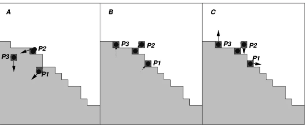
Bone dust, water and blood are modeled with a single particle system. Each parti-cle has a mass, a position, a velocity and a dynamic behavior. Water particles are intro-duced by the irrigator with an initial velocity directed along the irrigator axis. Dust par-ticles are generated by the burr performing the surgical bone drilling with an initial ve-locity depending on the rotation of the burr itself and a creation rate depending on the mass flux. Blood particles are generated by tissues with negligible initial speed. All par-ticles move according to Newton’s law when free, and interact with the other materials ac-cording to a set of rules that ensure that only a single particle may occupy a given voxel at given time. Basically, when a particle enters a non empty voxel, it is reflected backwards to the first free voxel. Its state is then mod-ified as a function of the colliding materials and the particle velocity (see figure 4).

When a particle collides with the environ-ment, we choose between elastic scattering or sliding along the bone surface based on the particle velocity. The random choice is made according to a probability distribution that favors scattering for high impact velocities. Different materials are modeled by shaping the probability distribution and by defining different particles masses and reflection co-efficients. In particular, bone particles have a behavior similar to water, but higher mass and higher probability to be scattered by hard bone.

We model bone paste formation by chang-ing the material of bone and water particles to “bone paste” when they collide.

We also consider the interaction of particles with the burr, by scattering away the particles

that enter in contact with the burr bit with a velocity depending on the rotational axis and speed of the burr.

Particles are deleted when they exit from the operation site.

5

Real–time visual rendering

The state of the simulation is entirely de-scribed by the contents of the rectilinear grid that contains the material labels used in the simulation. This also includes the particles modeling bone dust, debris and water. We provide real–time visual feedback in paral-lel with the simulation of the physical sys-tem with a direct volume rendering approach. Rendering such a dynamic volume under real-time constraints is particularly challenging. In our approach, a fast approximation of the diffuse shading equation [20] is computed on the fly by the graphics pipe-line directly from the scalar data. We do this by exploiting the possibilities offered by multi-texturing with the register combiner OpenGL extension, that provides a configurable means to determine per-pixel fragment coloring [1]. The extension is available on commodity graphics boards (e.g., NVIDIA GeForce series).

Object-aligned volume slices are composed back-to-front. The Lambert shading equa-tion is implemented in the graphics hard-ware by programming the register combiners, using multi-texturing to compute intermedi-ate slices and approximintermedi-ate opacity gradients with forward differences. Gradient norms, that provide “surface strength” [10], are com-puted using a second order approximation of the square root programmed with the regis-ter combiners. We refer the reader to [5], for more detail on the rendering technique.

This procedure is extremely efficient, since all the computation is performed in parallel in the graphics hardware and no particular synchronization is needed between the ren-derer and the process that is modifying the dataset. Only a single sweep through the

vol-ume is needed, and volvol-ume slices are sequen-tially loaded into texture memory on current standard PC graphics platform using AGP 4X transfers, which provide a peak bandwidth of 1054 MB/s.

6

System integration

Our technique for bone dissection simulation has been integrated in a prototype training system for mastoidectomy. We have exploited the difference in complexity and frequency requirements of the visual and haptic sim-ulations by modeling the system as a col-lection of loosely coupled concurrent compo-nents. Logically, the system is divided in a “fast” subsystem, responsible for the high fre-quency tasks (surgical instrument tracking, force feedback computation, bone erosion), and a “slow” one, essentially dedicated to the production of data for visual feedback. The “slow” subsystem is responsible for the global evolution of the water, bone dust and bone paste. The algorithms used to control the simulations are local in character and they are structured so that they communicate only via changes in the relevant, local, substance den-sities. This arrangement leads naturally to a further break-up of the slow subsystem in components, each dedicated to the generation of a specific visual effect, and thus to a parallel implementation on a multiprocessor architec-ture. The system runs on two interconnected multiprocessor machines. The data is initially replicated on the two machines. The first is dedicated to the high-frequency tasks: hap-tic device handling and bone removal simula-tion, which run at 1 KHz. The second con-currently runs, at about 15–20 Hz, the low-frequency tasks: bone removal, fluid evolution and visual feedback. Since the low-frequency tasks do not influence high-frequency ones, the two machines are synchronized using one-way message passing, with a dead reckon-ing protocol to reduce communication band-width.

Figure 5: The voxel based particle collision detection: each particle simulation step is subdivided in three sub-steps. First (subfigure A), particles are moved to target points according to their velocities; then (subfigure B), collisions with voxels containing bone or other particles are handled by moving colliding particles back to the first empty voxel; finally (subfigure C), scattering rules determine the new velocities assigned to the particles.

Figure 8: The virtual surgical setup

7

Implementation and results

Our current configuration is the following (see fig. 8):

• a single-processor PII/600 MHz with 256 MB PC133 RAM for the high-frequency tasks; two threads run in parallel: one for the haptic loop (1KHz), and one for sending volume and instruments position updates to the other machine;

• a dual-processor PIII/600 MHz with 512 MB PC800 RAM and a NVIDIA GeForce

3 Ti 500 and running a 2.4 linux ker-nel, for the low frequency tasks; three threads are continuously running on this machine: one to receive volume and po-sition updates, one to simulate bone re-moval and fluid evolution, and one for vi-sual rendering;

• a Phantom Desktop haptic device for the dominant hand; the device is connected to the single processor PC. It provides 6DOF tracking and 3DOF force feedback for the burr/irrigator;

• a Phantom 1.0 haptic device for the non-dominant hand; the device is connected to the single processor PC. It provides 6DOF tracking and 3DOF force feedback for the sucker;

• an n-vision VB30 binocular display for presenting images to the user; the binoc-ulars are connected to the S-VGA output of the dual processor PC.

The performance of the prototype is suffi-cient to meet timing constraints for display and force-feedback, even though the compu-tational and visualization platform is con-structed from affordable and widely accessible components. We are currently using a volume

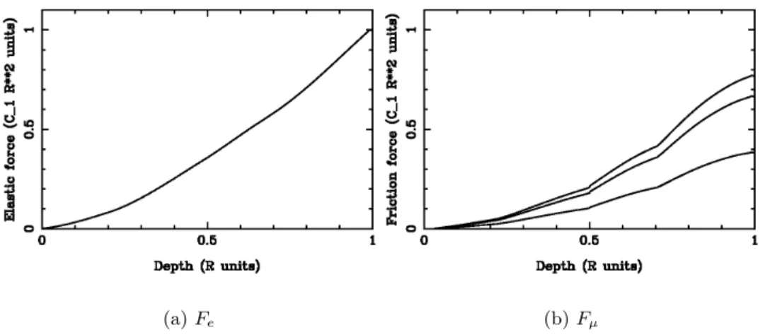
(a)Fe (b)Fµ

Figure 6: Virtual bone reaction against burr penetration. The computations are done in absence of erosion, α = ∞, using the actual force evaluation kernel of the force–feedback loop. In (a) we show the “elastic” response of the material, measured in units of C1R2,

as a function of the burr tip penetration depth in units of the burr bit radius R. Fig. (b) illustrates the “frictional” response of the material, with µ = 1/2 and for different angles

θ, θ = 30◦,60◦,90◦, between the surface normal and ωˆ. The strength of Fµ increases for

increasing sin(θ). The knees in the Fµ curves correspond to the intersection of the burr bit

with a deeper bone voxel layer.

of 256x256x128 cubical voxels (0.3 mm side) to represent the region where the operation takes place. The force–feedback loop is run-ning at 1 KHz using a 5x5x5 grid around the tip of the instruments for force computations. The computation needed for force evaluation and bone erosion takes typically 20µs, and less than 200µs in the worst case configuration.

In the following we will report on a series of experiments done using the prototype de-scribed above.

7.1 Force Evaluation

Figure 6 shows the reaction of the virtual bone against burr penetration. The computations are done in absence of erosion, α = ∞, and using the actual force evaluation kernel of the force–feedback loop.

Figure 6(a) illustrates the “elastic” re-sponse of the material, measured in units of

C1R2, as a function of the burr tip penetration depth measured in units of the burr bit radius

R. Figure 6(b) illustrates the “frictional”

re-sponse of the material, with µ= 1/2 and for different angles θ, θ = 30◦,60◦,90◦, between the surface normal andωˆ. The strength ofFµ

increases for increasing sin(θ). The knees in the Fµ curves correspond to the intersection

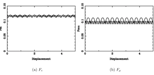
of the burr bit with a deeper bone voxel layer. Figure 7 shows the reaction of the virtual bone, again in runs withα =∞, to a sliding motion of the burr bit, immersed at a depth of R/4, over a flat bone surface. Fig. 7(a,b) show, respectively, the “elastic” and the “fric-tional” force response of the material, mea-sured in units of C1R2, as a function of the

distance traveled along the plane measured in

R units. The pair of curves in each figure correspond to a sliding motion over a bone surface aligned along, respectively, one of the voxel discretization axis, and a plane with normal [0,√1

2, 1 √

2]. The fluctuations in the

force values are due to the “voxel sphere” ap-proximation used to compute F. The differ-ence in the wavelength of the fluctuations is a factor of√2 as expected.

(a)Fe (b)Fµ

Figure 7: Sliding motion, constrained experiment. The reaction of the flat surface of virtual bone to the sliding motion of a burr bit immersed at a depth of R/4. Fig. (a,b) show, respectively, the “elastic” and the “frictional” force response of the material, measured in units ofC1R2, as a function of the distance traveled along the plane measured inRunits. The pair of curves in each figure correspond to a sliding motion over a bone surface aligned along, respectively, one of the voxel discretization axis, and a plane with normal [0,√1

2, 1 √

2]. The

fluctuations in the force values are due to the “voxel sphere” approximation used to compute

F. The difference in the wavelength of the fluctuations is a factor of√2 as expected. 7.2 Bone erosion

Figure 9 illustrates a “free–hand” experiment where bone is eroded by a polishing move-ment. The movement is similar to the one described in the previous subsection, with a sliding speed of about 10mm/sec, and α = 3.1 ×106mm2/sec2. Figure 9(a) shows the depth of the burr below the surface level as a function of time, while fig. 9(b) reports the components of the force contributions and the total force applied to the haptic display dur-ing the movement.

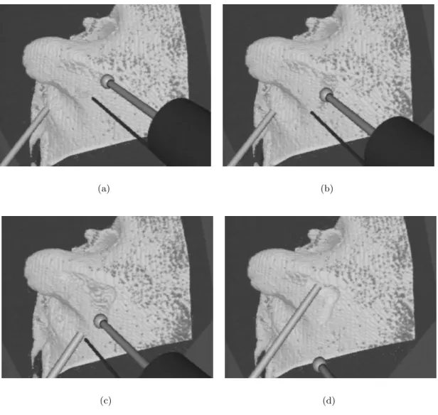
We have gathered initial feedback about the prototype system from specialist surgeons from the University of Pisa who are collab-orating with us in this research. Subjective input is being used to tune the parameters that control force feedback. The overall real-ism of the simulation is considered sufficient for training purposes. Fig. 10 shows a typical erosion sequence. A demonstration movie is available on the IERAPSI project web site [3].

8

Conclusions

and

Future

Work

We have presented a physically motivated haptic and visual implementation of a bone cutting burr, that is being developed as a component of a training system for temporal bone surgery. The current implementation, directly operating on a voxel discretization of patient-specific 3D CT and MR imaging data, is efficient enough to provide real–time multimodal feedback on a low–end multi– processing PC platform. In order to further improve the efficiency of the simulation, we are currenlty working on evaluating interac-tion forces using hierarchical techniques.

While subjective input from selected end users is encouraging, it would be of extreme interest to compare our results with direct forces measurements obtained by drilling ac-tual samples. Since, to our knowledge, there are no available data on the subject in litera-ture, we are currently defining an

experimen-(a) Depth (b) Forces

Figure 9: Bone erosion, polishing movement. A “free–hand” experiment where bone is eroded by a polishing movement. The sliding speed is about 10mm/sec, andα= 3.1×106mm2/sec2. Fig. (a) shows the depth of the burr below the surface level as a function of time. Fig. (b) reports the components of the force contributions and the total force applied to the haptic display during the movement. The lower line is the friction force F~µ, the middle line is the

elastic forceF~el, and the upper line is the total forceF~tot.

tal setup and measurement procedures. In our simulator, we are currently using datasets that have the same resolution as the original medical imaging data, and we are not differentiating between compact and trabecu-lar bone. It is our intention to explore the possibility of running the simulator on syn-thetically refined datasets obtained by using sub–voxel trabecular bone modeling.

9

Acknowledgments

We thank Pietro Ghironi, CRS4 technical ser-vices, for his support in setting up the surgical simulator hardware platform, and Alan Schei-nine for reviewing the manuscript.

These results were obtained within the framework of the European Union IERAPSI project (EU-IST-1999-12175).

References

[1] OpenGL extensions registry. Available

from http://oss.sgi.com/projects/ogl-sample/registry/.

[2] R. Adams and B. Hannaford. Stable hap-tic interaction with virtual environments.

IEEE Transactions on Robotics and Au-tomation, 15(3):465–474, 1999.

[3] M. Agus, F. Bettio, A. Giachetti, E. Gob-betti, G. Zanetti, and A. Zorcolo. Real– time haptic and visual simulation of bone dissection. Video demonstration, http://www.crs4.it/ierapsi, 2001.

[4] M. Agus, A. Giachetti, E. Gobbetti, G. Zanetti, N. W. John, and R. J. Stone. Mastoidectomy simulation with combined visual and haptic feedback. In J. D. Westwood, H. M. Hoffmann, G. T. Mogel, and D. Stredney, editors,

Medicine Meets Virtual Reality 2002, pages 17–23, Amsterdam, The Nether-lands, Jan. 2002. IOS Press.

[5] M. Agus, A. Giachetti, E. Gobbetti, G. Zanetti, and A. Zorcolo. A

multi-(a) (b)

(c) (d)

Figure 10: A virtual burring sequence. Here we show a typical bone cutting sequence per-formed in the mastoid region. The accumulation of debris, and its masking effects, is clearly visible.

processor decoupled system for the sim-ulation of temporal bone surgery. Com-puting and Visualization in Science, 5(1), 2002.

[6] M. Agus, A. Giachetti, E. Gobbetti, G. Zanetti, and A. Zorcolo. Real-time haptic and visual simulation of bone dis-section. In IEEE Virtual Reality Con-ference, pages 209–216, Conference held in Orlando, FL, USA, March 24–28, Feb. 2002.

[7] R. S. Avila and L. M. Sobierajski. A haptic interaction method for volume vi-sualization. InProceedings of the confer-ence on Visualization ’96, pages 197–204. IEEE Computer Society Press, 1996. [8] J. Colgate. Issues in the haptic display

of tool use. In Proceedings of ASME Haptic Interfaces for Virtual Environ-ment and Teleoperator Systems, pages 140–144, 1994.

Real time volumetric deformable models for surgery simulation. In VBC, pages 535–540, 1996.

[10] R. A. Drebin, L. Carpenter, and P. Han-rahan. Volume rendering. Computer Graphics, 22(4):51–58, August 1988. [11] R. Ellis, N. Sarkar, and M. Jenkins.

Nu-merical methods for the force reflection of contact. ASME Transactions on Dy-namic Systems, Modeling, and Control, 119(4):768–774, 1997.

[12] S. F. Frisken-Gibson. Using linked vol-umes to model object collisions, deforma-tion, cutting, carving, and joining. IEEE Transactions on Visualization and Com-puter Graphics, 5(4):333–348, Oct./Dec. 1999.

[13] T. A. Galyean and J. F. Hughes. Sculpt-ing: an interactive volumetric modeling technique. In Proceedings of the 18th annual conference on Computer graph-ics and interactive techniques, pages 267– 274. ACM Press, 1991.

[14] S. Gibson. Volumetric object modeling for surgical simulation, 1998.

[15] T. He and A. Kaufman. Collision detec-tion for volumetric objects. In Proceed-ings of the conference on Visualization ’97, pages 27–ff. ACM Press, 1997. [16] D. James and D. Pai. A unified

treat-ment of elastostatic contact simulation for real time haptics. Haptics-e, The Electronic Journal of Haptics Research (www.haptics-e.org), 2(1), September 2001.

[17] N. W. John, N. Thacker, M. Pokric, A. Jackson, G. Zanetti, E. Gobbetti, A. Giachetti, R. J. Stone, J. Campos, A. Emmen, A. Schwerdtner, E. Neri, S. S. Franceschini, and F. Rubio. An integrated simulator for surgery of the

petrous bone. In J. D. Westwood, edi-tor,Medicine Meets Virtual Reality 2001, pages 218–224, Amsterdam, The Nether-lands, January 2001. IOS Press.

[18] L. Landau and E. Lifshitz. Theory of elasticity. Pergamon Press, 1986.

[19] X. Li and J. Moshell. Modeling soil: Re-altime dynamic models for soil slippage and manipulation. In Computer Graph-ics Proceedings, Annual Conference Se-ries, pages 361–368, 1993.

[20] N. Max. Optical models for direct volume rendering.IEEE Transactions on Visual-ization and Computer Graphics, 1(2):99– 108, June 1995.

[21] W. A. McNeely, K. D. Puterbaugh, and J. J. Troy. Six degrees-of-freedom hap-tic rendering using voxel sampling. In A. Rockwood, editor,Siggraph 1999, An-nual Conference Series, pages 401–408, Los Angeles, 1999. ACM Siggraph, Ad-dison Wesley Longman.

[22] B. Pflesser, A. Petersik, U. Tiede, K. H. Hohne, and R. Leuwer. Volume based planning and rehearsal of surgical inter-ventions. In H. U. L. et al., editor, Com-puter Assisted Radiology and Surgery, Proc. CARS 2000, Excerpta Medica In-ternational Congress, 1214, pages 607– 612, Elsevier, Amsterdam, 2000.

[23] K. Shimoga. Finger force and touch feedback issues in dextrous telemanipu-lation. In Proceedings of NASA-CIRSSE International Conference on Intelligent Robotic Systems for Space Exploration, NASA, Greenbelt, MD, September 1992. [24] R. Sumner, J. O’Brien, and J. Hodgins. Animating sand, mud and snow. Com-puter Graphics Forum, 18:1, 1999. [25] S. W. Wang and A. E. Kaufman.

symposium on Interactive 3D graphics, pages 151–ff. ACM Press, 1995.

[26] G. Wiet, J. Bryan, D. Sessanna, D. Streadney, P. Schmalbrock, and B. Welling. Virtual temporal bone dissec-tion simuladissec-tion. In J. D. Westwood, edi-tor,Medicine Meets Virtual Reality 2000, pages 378–384, Amsterdam, The Nether-lands, January 2000. IOS Press.