Volume 64 (2013)
Proceedings of the
XIII Spanish Conference on Programming
and Computer Languages
(PROLE 2013)
On the decidability of model checking LTL fragments in monotonic
extensions of Petri nets
Mar´ıa Martos-Salgado and Fernando Rosa-Velardo
18 pages
Guest Editors: Clara Benac Earle, Laura Castro, Lars- ˚Ake Fredlund Managing Editors: Tiziana Margaria, Julia Padberg, Gabriele Taentzer
On the decidability of model checking LTL fragments in monotonic
extensions of Petri nets
Mar´ıa Martos-Salgado1and Fernando Rosa-Velardo2∗
Universidad Complutense de Madrid
Universidad Complutense de Madrid
Abstract: We study the model checking problem for monotonic extensions of Petri Nets, namely for two extensions of Petri nets: reset nets (nets in which places can be emptied by the firing of a transition with a reset arc) andν-Petri nets (nets in which tokens are pure names that can be matched with equality and dynamically created). We consider several fragments of LTL for which the model checking problem is decidable for P/T nets. We first show that for those logics, model checking of reset nets is undecidable. We transfer those results to the case ofν-Petri nets. In order to cope with these negative results, we define a weaker fragment of LTL, in which negation is not allowed. We prove that for that fragment, the model checking of both reset nets andν-Petri nets is decidable, though with a non primitive recursive complexity. Finally, we prove that the model checking problem for a version of that fragment with universal interpretation is undecidable even for P/T nets.
Keywords: LTL, model checking, Petri nets, decidability, complexity
1
Introduction
Temporal logics [4] have been established as a very expressive formalism for the specification of properties of computational concurrent systems. Model checking is the problem of deciding if a given system satisfies a given temporal formula.
For infinite state systems the model checking problem is undecidable in general [15]. A very well known formalism for infinite state concurrent systems is that of Petri nets [6]. Among them, place/Transition nets (P/T nets) are potentially infinite state, but their expressive power is be-low Minsky machines (e.g., reachability is decidable for them [8]). Decidability and complexity of the model checking problem for P/T nets are well studied, and the corresponding decidability frontiers are well settled [13,9,12,8]. Roughly speaking, model checking of P/T nets is undecid-able for any branching-time logic, while for linear time logics, “event-based” LTL is decidundecid-able, though “state-based” LTL is undecidable.
In the last two decades, several monotonic extensions of Petri nets have appeared in the lit-erature. These extensions usually consist either on the extension of the firing rule of P/T nets,
∗ Authors supported by the Spanish projects STRONGSOFT TIN2012-39391-C04-04 and PROMETIDOS
or on the use of colours, that is, distinguishable tokens. We consider two simple extensions of P/T nets, one in each group: reset nets [7] andν-Petri nets (ν-PN) [21]. In reset nets the firing of a transition can empty some places. Their modeling capabilities are discussed for instance in [14]. Tokens in ν-PNs are pure names, that can be created fresh, moved along the net and used to restrict the firing of transitions with name matching. Names can be seen as process identifiers [19], so thatν-PN can serve as the basis of models in which an unbounded number of components (which are in turn unbounded) synchronize. For example, they can be used to model resource-constrained workflow nets, an extension of workflow nets in which an arbitrary number of instances of the workflow can be executed concurrently [11]. In [5], they are used to give a semantics to an extension of BPEL [16] with instance isolation.
In this paper we study the decidability of the model checking problem of these models. More precisely, we consider the logics for which model checking of P/T nets is decidable, and we study their decidability for the two extensions. In particular, we study LT Lf, which is the fragment of LTL that uses only first as basic predicate [9],L(F), the fragment of LTL in which negation is
only applied to basic predicates (not to operators), and the operators are X (next), F (eventually), ∧and∨[12]; andL(GF), which is the fragment of LTL in which the only allowed composed
operator is GF (globally future), the operators are F,∨and∧and negation is only applied to basic predicates [13].
Unfortunately, we conclude that the decidability results for P/T nets cannot be adapted, so that model checking for any of the logics considered is undecidable. In particular, we reduce LT Lf model checking of lossy inhibitor nets, which is undecidable, to LT Lf model checking of reset nets. Moreover, we prove that repeated coverability and reachability, which are undecidable for reset nets, can be expressed inL(GF)andL(F)respectively.
As a first step to mitigate the previous undecidability result, we consider a fragment of LTL weaker than all the logics considered so far in which, in particular, we do not allow negations. We call that logic Fcov. We prove that the model checking problem for this logic is decidable for both models.
In some of the subclasses of LTL considered in the literature [13,12] a formula is said to be satisfied if there exists one run that satisfies it, as opposed to the more standard definition of LTL in which all runs are required to satisfy the formula. Even though the two interpretations are equivalent when negation can be used without restriction, this is not the case for the considered subclasses of LTL, neither for Fcov. We justify this definition by proving that already for P/T nets, Fcov model checking is undecidable under the universal interpretation.
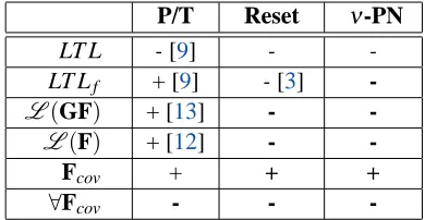
Table1summarizes the results on model checking of P/T nets, reset nets andν-PNs. By “+” (resp. -) we denote that the model checking problem for the considered logic is decidable (resp. undecidable). If the references of the results are not given, then the result is either new (the ones with signs in bold letters) or follows directly from other results of the table.
P/T Reset ν-PN
LT L - [9] - -LT Lf + [9] - [3] -L(GF) + [13] - -L(F) + [12] -
-Fcov + + +
∀Fcov - -
-Table 1: Summary of results. Those in bold signs are the new contributions of this paper.
2
Preliminaries
A quasi order (qo) is a reflexive and transitive binary relation. For a qo≤, we write a<b if a≤b and b6≤a.
Labelled transition systems. A transition system is a tupleS = (S,L,→,init), where S is a
(possibly infinite) set of states, L is a set of labels, init∈S is the initial state and→⊆S×L×S1. Given two states s1,s2∈S and a∈L, we write s1
a
→s2instead of(s1,a,s2)∈→, and s1→s2 if s1
b
→s2for some b∈L. We denote by→∗the reflexive and transitive closure of→and by→+
the transitive closure of→. A runπ ofS is any sequence s0
a0 →s1
a1
→s2...such that si ai →si+1
for i≥0. We define the length of a run π as n∈Nif π=s0→a0 s1→a1 ...→an sn is a finite run, and∞ifπ is an infinite run. The reachability problem consists in deciding for a given state sf whether init →∗s
f. If S is endowed with a qo≤we can define the coverability problem, that consists in deciding, given sf ∈S, whether some s≥sf is reachable. Then, we say that s covers
sf. The repeated coverability problem is the problem of deciding whether a given state is covered infinitely often in some infinite run starting in init, that is, for a given s there is an infinite run
init→+s1→+s2→+...such that s≤sifor all i≥1.
Multisets. Given a (possibly infinite) arbitrary set A, we denote by A⊕the set of finite multisets over A, that is, the mappings m : A→Nfor which supp(m) ={a∈A|m(a)>0}is finite. When needed, we identify each conventional set with the multiset defined by its characteristic function, and use set notation for multisets when convenient, with repetitions to account for multiplicities greater than one. Moreover, given two sets A and B, and an injection α : A→B, sometimes
we interpretα as the functionα : A⊕→B⊕ such that given MA∈A, α(MA) =MB, where for each b∈B, MB(b) =n>0 if there exists a∈A withα(a) =b and MA(a) =n, and MB(b) =0 otherwise.
Given two multisets m1,m2∈A⊕we denote by m1+m2the multiset defined by(m1+m2)(a) = m1(a) +m2(a). We define multiset inclusion as m1⊆m2 if m1(a)≤m2(a) for all a∈A. If m1⊆m2, we can define m2−m1, taking(m2−m1)(a) =m2(a)−m1(a). We denote by /0∈A⊕
the empty multiset, given by /0(a) =0 for all a∈A.
Petri nets. A Place/Transition net (P/T net for short) is a tuple N= (P,T,F)where P is a finite set of places, T is a finite set of transitions (with P∩T =/0) and F :(P×T)∪(T×P)→Nis
• a •
a b
••
p q
r t
→
• a •
a
•
p q
r t
Figure 1: The firing of a transition in a P/T net.
the flow function. Given t∈T , the multiset of preconditions of t is•t∈P⊕ given by(•t)(p) = F(p,t). Analogously, the postconditions of t are given by(t•)(p) =F(t,p). A marking is any
m∈P⊕. For Petri nets we consider the order between markings given by multiset inclusion. This order defines the standard coverability problem for Petri nets. We say that a transition t is enabled at a marking m if for each p∈P, m(p)≥F(p,t). In that case, t can be fired from m, reaching a new marking m′, which is denoted by m→t m′, where m′is given by m′(p) = (m(p)−
F(p,t)) +F(t,p). The reachability, the coverability and the repeated coverability problems are all decidable for P/T nets [8]. In the rest of this paper, we represent places as circles, transitions as rectangles, the flow function as arrows and markings as tokens inside places. The arcs which represent the flow function are not labelled by any constant representing the corresponding values of F. That is because for all p∈P, t∈T with an arc going from p to t (resp. from t to p) in
figures, we assume F(p,t) =1 (resp. F(t,p) =1).
Example 1 In the P/T net in the left-hand side of Fig.1, transition t is enabled, so it can be fired reaching the marking depicted in the right-hand side. Tokens have been consumed from p and r, and a token has been produced in q. As there is not a priority order over transitions, note that from the marking represented in the left-hand side, the other transition could have been fired instead of t, reaching a marking with a token in each place of the net.
Now, we explain two extensions of P/T nets, namely reset nets and inhibitor nets. Both of them are defined from P/T nets by adding special arcs: reset arcs, which empty a place, and inhibitor arcs, which add to the enabling conditions the requirement that a certain place is empty. For both extensions, the concepts of preconditions, postconditions and marking are analogous to those for P/T nets.
A reset net is a tuple N= (P,T,F,R), where(P,T,F)is a P/T net and R⊆P×T is a relation
containing the so called reset arcs. The enabled transitions at a marking are defined as for P/T nets. An enabled transition t can be fired from a marking m reaching m′given by:
m′(p) =
(m(p)−F(p,t)) +F(t,p) if(p,t)∈/R F(t,p) if(p,t)∈R
Notice that if (p,t)∈R and F(t,p) =0 (i.e., t does not put any token in p) then p has no tokens after the firing of t (hence p is reset).
Example 2 Focus on Fig. 2. The double arc represents a reset arc from place r to t, that is,
• a •
a b
••
p q
r t′
t
→
• a •
a •
p q
r t′
t
Figure 2: The firing of a transition in a reset net.
ab ab
a
bc be
p1 p3
p2 p4
xy xν1
y ν1ν2
→
aa ad
a
c de
(d,e fresh)
p1 p3
p2 p4
xy xν1
y ν1ν2
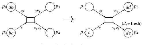
Figure 3: A simpleν-PN
of the figure, and it can be fired, reaching the marking depicted in the right. All tokens in place r have been consumed in the firing of t due to the presence of the reset arc. Note that transition t′ is also enabled in the marking represented in the net in the left-hand side. Transitions with reset arcs do not have any priority over the rest of the enabled ones. Therefore, transition t′could be fired from the first marking too.
An inhibitor net is a tuple N= (P,T,F,I)where N= (P,T,F)is a P/T net, and I⊆P×T is a
relation containing the inhibitor arcs (also called zero tests). We say that a transition t is enabled at a marking m if:
• for each p∈P, m(p)≥F(p,t)and
• for each(q,t)∈I, m(q) =0 (place q is empty).
Then, t can be fired from m, reaching the marking m′given by m′(p) = (m(p)−F(p,t)) +F(t,p)
(as for P/T nets) 2. Inhibitor nets with two inhibitor arcs are already Turing complete [15], though, interestingly, inhibitor nets with only one inhibitor arc are not [18].
ν-PN. Another way in which P/T nets are extended in the literature is by considering able tokens. Perhaps the most simple extension of P/T nets with (arbitrarily many) distinguish-able tokens areν-Petri Nets [21], that encompass unboundedly many names (via a mechanism for fresh name creation) and the unbounded occurrence of each name.
Let Var be a set of variables, andϒ⊂Var a set of special variables for fresh name creation. A
ν-Petri Net (ν-PN for short) is a tuple N= (P,T,F), where P and T are finite disjoint sets, and
F :(P×T)∪(T×P)→Var⊕ labels every arc by a multiset of variables. We denote pre(t) =
S
p∈Psupp(F(p,t))(the set of variables in pre-arcs) and post(t) =
S
p∈Psupp(F(t,p))(the set of variables in post-arcs). We also take Var(t) =pre(t)∪post(t).
2Actually, it is straightforward to simulate a reset arc using inhibitor arcs, in a way preserving reachability,
Let Id be an infinite set of names. A marking of aν-PN is a mapping M : P→Id⊕ assigning to each place the multiset of tokens currently in it. We take Id(M) =S
p∈Psupp(M(p)), that is, the set of names in M.
Given a transition t∈T of aν-PN, a mode for t is any injectionσt: Var(t)→Id. As modes are injections, we can match names with equality (just by using the same variable more than once) and with inequality (by using different variables). We say that a transition t is enabled with a modeσt for a marking M, if for eachν∈ϒ,σt(ν)∈/Id(M)and for all p∈P,σt(F(p,t))⊆M(p). Then, t can be fired, and a new marking M′is reached, given by M′(p) = (M(p)−σt(F(p,t))) +
σt(F(t,p))for all p∈P. In that case we write M t →M′.
Example 3 Fig.3depicts the ν-PN N given by N= ({p1,p2,p3,p4},{t},F) with F(p1,t) =
{x,y}, F(p2,t) ={y}, F(t,p3) ={x,ν1}, F(t,p4) ={ν1,ν2}, and for(n,m)∈ {(p3,t),(p4,t), (t,p1),(t,p2)}, F(n,m) = /0. We assume that ν1,ν2 ∈ϒ. The initial marking is given by M0(p1) ={a,b}, M0(p2) ={b,c}and M0(p3) =M0(p4) = /0. The transition is fired with
re-spect to a modeσ given byσ(x) =a,σ(y) =b,σ(ν1) =dandσ(ν2) =e. Note that names d
and e are not in the initial marking, and therefore they are created new.
Intuitively, each name in a marking of aν-PN can represent a different process running in the same net. Therefore, we can represent the synchronization between processes and the creation of new ones.
Given a marking M of a ν-PN and a set I of names, a renaming of M is any injection α :
Id(M)→I. We say that M⊑M′⇔there is a renamingα of M such thatα(M)(p)⊆M′(p)for all p∈P. With this order, coverability is decidable forν-PN, though reachability is undecidable for them [21].
Example 4 The marking M given by M(p1) =/0, M(p2) =/0, M(p3) ={a,d}, M(p4) ={a,c}
is covered by the marking M′on the right-hand side of Fig.3. Note that, although there is not a token of name a in place p4, with the order we have defined, M is covered by M′by considering
the renamingα, such thatα(a) =d,α(d) =aandα(e) =c.
Finally, note that both models induce labelled transition systems in the obvious way: the states of the labelled transition systems are the markings of the nets, the set of labels is the set of transitions, and ifM is the set of markings of the net, the transition relation→⊆M×T×M
is the one such that m1→t m2in the net⇔(m1,t,m2)∈→.
3
Model checking of Petri net extensions
with branching time logics is undecidable, even for very simple fragments [9].
The basic temporal operators used in temporal logics are X, F and U3. The most representative example of a linear time logic is LTL.
Definition 1 An LTL formula is either an atomic proposition or a formula of the form ¬ϕ, ϕ∧ψ,ϕ∨ψ, Xϕ, Fϕ, orϕUψ, whereϕandψ are LTL formulae.
First, we explain the semantics of the temporal operators informally. LTL formulae are inter-preted over maximal runs, i.e., runs that are either infinite, or end in a deadlock state. Letϕ be an LTL formula,S a transition system andπ a maximal run starting in s. We writeS,πϕto
denote thatπ satisfiesϕ:
• S,πXϕ(next) holds if the propertyϕ holds in the state that follows s inπ.
• S,πFϕ(eventually) holds if the propertyϕholds in some state ofπ.
• S,πϕUψ (until) holds if there is a state of the runπsuch thatψholds in that state, and
ϕholds at every preceding state on the run.
We also define G (globally) as Gϕ=¬F¬ϕ, so thatS,πGϕholds ifϕholds in every state
ofπ.
Now, we give the formal semantics of temporal operators. Letπ=s0→a1 s1→a2 . . .be a finite or infinite run of length n∈N∪ {∞}. For n>0,πiis defined as the suffix of the runπ starting by the i-th state si. We suppose that the states and the actions of a system are labelled by the atomic propositions that they satisfy, that is, if a state s (or an action a) satisfies an atomic proposition
p, then p∈L(s) (p∈L(a) resp.), where L(s)(L(a)) represents the labels of s (a). The formal definition of the semantics of the previous operators is inductively defined as [4]:
• T,πp⇔p∈L(s0)∨π1is defined (that is, the length ofπis greater than 0) and∈L(a1).
• T,π¬ϕ1⇔T,π2ϕ1.
• T,πϕ1∨ϕ2⇔T,πϕ1orT,πϕ2.
• T,πϕ1∧ϕ2⇔T,πϕ1andT,πϕ2.
• T,πXϕ1⇔π1is defined andT,π1ϕ 1.
• T,πFϕ1⇔there exists a k≥0 such thatT,πkϕ
1.
• T,πGϕ1⇔for all i≥0 such thatπiis defined,T,πiϕ1.
• T,π ϕ1Uϕ2 ⇔ there exists a k≥0 such that πk is defined, T,πk ϕ2 and for all
0≤j<k,T,πjϕ
1.
3Even though F can be defined in terms of U, we prefer to include it as a primitive temporal quantifier, since we will
Note that in the previous definition, we assign the propositions they satisfy to both the states and the transition labels (a), defined for the labelled transition systems. The atomic propositions usually considered for P/T nets, are given by the following predicates:
• cov(m), where m is a marking: cov(m)holds inπif the first marking inπcovers m.
• first(t), where t is a transition: first(t)holds inπif the first transition fired inπis t.
Some works consider the atomic propositions ge(p,n) and en(t)[9]. The first one expresses that there are at least n tokens in place p, and the second states that t is enabled. We will not consider them since they are equivalent to cov({p, ...,n p})and cov(•t), respectively.
According to the standard definition, a system S satisfies an LTL formulaϕ, denoted by
S |=ϕ iff every maximal run of the system starting in the initial state init satisfies it (universal interpretation). The model checking problem consists in deciding, given S and ϕ, whether S |=ϕ. The model checking problem is equivalent to deciding, givenS andϕ, the existence of
one run starting in init satisfying the formula (existential interpretation), provided negation can be used without restriction, since S|=ϕ (under the universal interpretation) iff S6|=¬ϕ (under the existential interpretation).
We consider different LTL fragments, built depending on which predicates and operators we consider.
Definition 2 We consider the following fragments of LTL:
• LT Lf, the fragment of LTL that uses only first as basic predicate [9],
• L(F), the fragment of LTL in which negation is only applied to basic predicates (not to operators), and the operators are X, F,∧and∨[12],
• L(GF), the fragment of LTL in which the only allowed composed operator is GF, the
operators are F,∨and∧and negation is only applied to basic predicates [13].
Example 5 The formula Ffirst(t), which expresses that t is eventually fired, is inL(F), but Gfirst(t) =¬F¬first(t), which expresses that t is always fired, is not.
The formula first(t)→GFfirst(t), which expresses that if t is the first transition being fired then t is fired infinitely often, is inL(GF), but Ffirst(t)→GFfirst(t) =¬Ffirst(t)∨GFfirst(t),
which expresses that if t is eventually fired, then it is fired infinitely often, is not.
In LT Lf negation can be used without restriction, so that the universal and the existential inter-pretations are equivalent (i.e., their model checking decision problems are equivalent). However, this is not the case forL(F)andL(GF). Actually, they are defined using the existential
inter-pretation in [12,13]. For the subclasses of LTL considered, we have the following results.
• LTL model checking is undecidable (with both first and cov), but LT Lf model checking is decidable (with cov only) [9].
• L(F)model checking is decidable [12] (with existential interpretation),
3.1 Model checking of reset nets
Let us show that the three logics which are decidable for P/T nets become undecidable for reset nets. Let us first consider LT Lf. In [3] the model checking problem of LT Lf is studied for lossy vector addition systems (lossy VAS) with tests for zero, which is proved to be undecidable. Let us see that we can adapt that result for reset nets. Let us first define the lossy version of a transition system in general.
Definition 3 Given a transition systemS = (S,→,init)and a quasi-order≤over S, the lossy
version ofS isSl = (S,→l,init), where s1→ls2if and only if there exists two states s′1and s′2
such that s1≥s′1→s′2≥s2. A lossy Petri net is the lossy version of some Petri net.
In the lossy version of a transition system, states can be spontaneously decreased. In the case of Petri nets, tokens may be lost just before or after a transition is fired.
Example 6 Focus on Fig.2. In the lossy version of the P/T net obtained by replacing the reset arc by a plain arc, despite r is not reseted by any reset arc of t, the second marking could be reached from the first one by first losing a token from r and then firing t.
Reset nets can simulate lossy inhibitor nets, as we prove next. This fact is used in the proof of the next result.
Proposition 1 LT Lf model checking is undecidable for reset nets.
Proof. We reduce LT Lf model checking for lossy inhibitor nets, which is undecidable [3], to the same problem for reset nets. Let N= (P,T,F,I) be an inhibitor net. We define the reset net N′= (P,T,F,I). We are going to prove that there is a surjective function between the runs of N and N′ that preserves the sequence of labels of runs and therefore, since the only atomic proposition in LT Lf is first, given an LT Lf formulaϕ, N|=ϕiff N′|=ϕ. Notice that since N′is a reset net, checks for zero have been replaced by resets, that is, an inhibitor arc from a place p to a transition t in N is replaced by a reset arc from p to t in N′. The following holds:
• m1
t
→m2in N⇒there is an m′2≥m2such that m1
t
→m′2in N′: the preconditions and effects of the firings of t in N and N′ are the same, except for the fact that we have replaced inhibitor arcs by reset arcs. Therefore, when a transition with an inhibitor arc in N is firing in N′, the corresponding place is reseted instead of being checked for zero. If there are tokens in such a place, all the tokens in it are removed, so there exist a possibility of losing tokens in our simulation if the place was not empty. If t has no inhibitor arc, and m1→t m2
in N, t is enabled at m1in N′, and it can be fired reaching a marking greater or equal than m2, because some token may have been lost in the firing in N.
Now, suppose that t has some inhibitor arcs, and m1
t
→m2in N. First of all, note that if a transition is enabled in N at a marking, it is enabled in N′at the same marking. Moreover, the places with inhibitor arcs leading to t are empty in that marking. Therefore, when t is fired from m1 in N′, these places are reset (hence staying empty). Therefore, the only
t t • • t t t •• •• t t t • • t t t A1 A2 B1 B2 m1 m′
1 m′2
m21 m22
m1
m′
1 m′12
m2
m′ 21
m′ 22
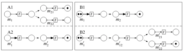
Figure 4: From lossy inhibitor nets to reset nets
particular, since t may loose tokens in N, but not in N′, m1
t
→m′2in N′, with m′2≥m2.
For example, focus on the left-hand side of Fig.4. In the inhibitor nets depicted in this figure, given a place p and a transition t, we represent(p,t)∈I by an arc from p to t, with
a circle in the place p. The marking m1in the first lossy inhibitor net in A1 may evolve to m21or m22(m22has lost the token). The corresponding reset net, depicted in A2 can only
evolve t the marking m′2. However, note that m′2covers both m21and m22.
• m1
t
→m2in N′⇒m1
t
→m2in N: In particular, if N′resets a place, N can first loose tokens,
thus emptying it, and then test for zero in that place. Therefore, the transition is fireable in N (because the preconditions of the firings of t in N and N′are the same, except for the lossiness and the inhibitor arcs) and the place is empty at the end of both firings.
Focus on the right-hand side of Fig.4. Transition t is fireable from the marking m1 in
the reset net in B1, reaching the marking m2. Despite t is not fireable from m′1=m1, the
lossy inhibitor net may lose tokens, reaching m′12, from which t can be fired, reaching the markings m′21or m′22.
Therefore, there is a surjective function between the runs of N and N′that preserves the sequence of labels of runs. Note that this holds because reset nets are monotonic, so transitions which are fired in N at a marking m which has lost tokens, can be fired from the corresponding marking m′ of N′, without loss of tokens, because m′≥m. Since the only atomic proposition in LT Lf is first,
N|=ϕiff N′|=ϕand we conclude.
Let us now focus on the two other fragments of LTL. The case forL(GF)is straightforward:
Proposition 2 L(GF)model checking of reset nets is undecidable.
However, not only that fragment, but the weaker fragmentL(F), which is decidable for P/T
nets [12], is undecidable for reset nets. The following proof uses ideas from [12], in whichL(F)
model checking is reduced to reachability for P/T nets.
Proposition 3 L(F)model checking of reset nets is undecidable.
Proof. We reduce reachability, which is undecidable for reset nets [2], to model checking some formula inL(F). Let N= (P,T,F,R)be a reset net and m a marking of N. We can compute the set of the least markings greater than m.4Indeed, that set is just{mp|p∈P}, where mpis given by mp(q) =m(q)for q=6 p and mp(p) =m(p) +1. For example, the set of the least markings greater than the marking depicted in the net in the left-hand side of Fig.2is{mp,mq,mr}, where
mp={p,p,r,r}, mq={p,q,r,r} and mr={p,r,r,r}. Then, m is reachable in N iff there is a reachable marking m′ that covers m, but does not cover any mp, because this would imply that in each place p, m′ has exactly m(p) tokens (because it does not cover mp). Therefore, m is reachable in N iff the formula F(cov(m)∧V
p∈P¬cov(mp))is satisfied.
The previous proof is based on obtaining a formula which expresses the reachability problem. In order to obtain this formula, there is an important property that reset nets satisfy: Given a marking m, we are able to compute a finite set of markings S={m1, . . . ,mn}such that for each
mi∈S, mi⊃m and if m′⊃m, then there is mi∈S such that m′⊇mi. Intuitively, we can compute the finite set of “the smallest markings greater than m”. As we can build that set, a marking mf coincides with m if and only if mf covers m and mf does not cover any marking of S.
3.2 Model checking of
ν
-PNWe first recall from [21] howν-PN can simulate reset nets (see Fig.5, where the double arrow represents a reset arc). For each place p of a reset net N we consider a copy of it and a new place
p′ in theν-PN N′ we build. The main idea of the construction is to store in place p′ a single token of the colour that we consider valid in the current marking for place p of N′. That is, the tokens in p of the colour of the token in p′ will be considered valid, and the rest of the tokens in
p will be considered garbage. For example, in theν-PN of Fig.5, there are two valid tokens in place r, because the colour of the token in r′is b.
The construction of N′ guarantees that for each place p of N, the place p′ of N′ contains a single token at any time. The firing of any transition ensures that the token being used in the place p of N′ coincides with that in p′(by labelling both arcs with the same variable xp). Every time a transition resets a place p of N, the token in p′is replaced by a fresh one, so that no token remaining in place p of N′ can be used from then on. For example, suppose we fire transition t in Fig.5. Then, a new colour is put in r′, and therefore the tokens of name b in r cannot be used anymore.
Therefore, this simulation can introduce some garbage tokens (those in p when p is reset). Given a marking m we define m′by arbitrarily choosing a different name ap∈Id for each p∈P, and taking m′(p′) ={ap}, and m′(p) ={ap,m(p)... ,ap}. Then, if m0is the initial marking of N, N′
• a •
a b
••
p q
r t
→
a a aa c
c bb b
a
p q
r
p′
r′
q′
t
xp xq
xp xq
xr ν
xr
xq
xq
xr
Figure 5: A reset net and the correspondingν-PN. The double arrow represents a reset arc
with initial marking m′0simulates N. The previous simulation preserves all behavioral properties. Then, the following is a straightforward consequence of Prop.1.
Corollary 1 LT Lf model checking is undecidable forν-PN.
The previous simulation also preserves coverability. More precisely, if a marking m is cover-able in the reset net N, then the marking m′of N′ defined above is coverable too. The markings in the simulation may contain some garbage, which is created when we simulate the firing of a reset, because instead of removing all tokens of some place p, we change the name of the token in p′, making all tokens in p become garbage. However, the presence of that garbage is irrelevant for coverability. In particular, we have the following.
Proposition 4 Repeated coverability is undecidable forν-PN.
Proof. It is enough to consider that repeated coverability is undecidable for reset nets [2], and that the previous simulation preserves repeated coverability. We prove that m can be repeatedly covered from m0in N iff M′can be repeatedly covered from m′0in N′. Indeed, if m is repeatedly
covered there is a run m0→+m1→+m2→+...of N such that mi≥m for all i≥1. By construc-tion of N′, there is a run m′0→+M1→+M2→+ ...of N′ such that Mi≥m′i≥m′ for all i≥1, so m′ is repeatedly covered. Moreover, Mi coincides with m′i when considering only the “valid tokens” of Mi (and after possibly renaming the names carried by the tokens). The converse is analogous.
Once we know that repeated coverability is undecidable, undecidability of L(GF) model checking is trivial.
Corollary 2 L(GF)model checking ofν-PN is undecidable.
Next, we see the undecidability ofL(F)model checking forν-PN.
Proposition 5 L(F)model checking ofν-PN is undecidable.
Proof. The proof is analogous to the one of the same result for reset nets. We reduce reachability
Mpc given by Mpc(q) =M(q)if p=6 q and Mpc(p) =M(p) +{c}. Then, the set we are looking for is{Mpc|p∈P,c∈Id(M)∪ {b}}. For example, consider a net with two places p and q, and a marking M with one token a in p and empty in q. The set of the least markings greater than this marking is {Mpa,Mpb,Mqa,Mqb}, where Mpa(p) ={a,a}, Mpa(q) = /0, Mpb(p) ={a,b},
Mpb(q) = /0, Mqa(p) ={a}, Mqa(q) ={a}, Mqb(p) ={b}and Mqb(q) ={a}. Therefore, M is reachable in N iff N|=F(cov(M)∧V
p,c¬cov(Mpc)), and we conclude.
4
A decidable fragment
In the previous section we have proved the undecidability of model checking of reset nets and ν-PN for some logics, whose model checking problem is known to be decidable for P/T nets. In this section we define a restriction ofL(F), thus obtaining a fragment that is less expressive
than all the logics considered here.
Definition 4 Fcovis the fragment ofL(F)in which negation is not allowed.
In this logic we can express bounded repeated coverability. However, Fcov cannot express properties like ¬cov(M). In particular, the formula F(cov(M)∧V
p∈P¬cov(Mp)) which ex-presses reachability, is not a formula of Fcov. As forL(F), we consider existential interpretation, so that a formula is satisfied if some maximal run starting in the initial marking satisfies it. We will see that Fcov model checking is decidable both for reset nets and forν-PN. Later, we will consider ∀Fcov, the version of Fcov with universal interpretation, and we will prove that ∀Fcov model checking is undecidable even for P/T nets.
Proposition 6 Fcovmodel checking of reset nets is decidable.
Proof. Let N= (P,T,F,R)be a reset net andφ a formula in Fcov. We proceed by induction on the nesting of operators F inφ. Ifφis a boolean combination of formulae of the form cov(m), it is trivial to decide whetherφ is satisfied because multiset inclusion is decidable.
Let us suppose that we can check each formula with at most n>0 nested F operators. Let φ be a boolean combination of formulae of the form cov(m) and Fϕ, where ϕ has at most
n nested F operators, and let us see that we can decide whether each of those formulae Fϕ
is satisfied (and hence, whether φ is satisfied). Using standard techniques, we can write Fϕ as F(W
i((
V
jcov(mi j))∧(VkFϕik))), whereϕik are formulae of Fcov with at most n−1 nested operators. That formula is equivalent to the formulaW
iF((
V
jcov(mi j))∧(VkFϕik)), that is, a disjunction of formulae of the form F(cov(m1)∧...∧cov(mq)∧Fϕ1∧...∧Fϕr), where q and r are not simultaneously zero, and eachϕk has at most n−1 nested operators. Let us distinguish the following two cases:
(a) If q=0 the formula is of the form F(Fϕ1∧...∧Fϕr), which is equivalent to Fϕ1∧...∧Fϕr. Hence, we can apply the induction hypothesis to each Fϕkand we are done.
(b) If q>0, we modify N, thus obtaining N′, by adding transitions t1, ...,tq,tq+1 and places p0,p1, ...,pqas follows. We add p0as precondition/postcondition of every transition in N.
More-over, ti moves a token from pi−1 to pi, provided mi is covered. Finally, tq+1 can be fired only
p0 t1
p1 p2
t2
•
paux
t3
m
1m
2N
Figure 6: Construction of N′in Prop.6
setting again a token in p0, and having pqas precondition and postcondition. This construction is represented in Fig.6, for q=2. Then, N′ behaves as N, but when every mi can be covered, it can sequentially fire t1, ...,tq,tq+1. Hence, every mican be simultaneously covered in N iff pq can be covered in N′. We consider the following two sub-cases:
(b.1) If r=0 then the formula is of the form F(cov(m1)∧...∧cov(mq))and hence equivalent to Fcov({pq}), which expresses a coverability problem, so that it can be decided.
(b.2) Consider now that r>0. For any formulaϕ, we defineϕ′as follows:
• Ifϕ=cov(m)thenϕ′=cov(m+{pq}).
• Ifϕ=ϕ1∧ϕ2thenϕ′=ϕ1′∧ϕ2′. Analogously, ifϕ=ϕ1∨ϕ2thenϕ′=ϕ1′∨ϕ2′.
• Ifϕ=Fϕ1thenϕ′=Fϕ1′.
Then, F(cov(m1)∧. . .∧cov(mq)∧Fϕ1∧. . .∧Fϕr)holds in N iff F(Fϕ1′∧. . .∧Fϕr′)holds in
N′. Notice that the number of nested F operators is the same forϕkandϕk′. Then, by (a) we are done.
The proof of the same result forν-PNs is analogous to the previous one.5
Proposition 7 Fcovmodel checking is decidable forν-PN.
Proof. The construction forν-PN is the same as the previous one. The only difference is that the names in the markings of the formulae need to be handled correctly in N′, by choosing a different variable for each name in a marking to label the arcs.
Since in particular Fcov allows us to express coverability, which has a non primitive recursive complexity for reset nets [22] and forν-PN [21], we have the following:
Proposition 8 The complexity of Fcovmodel checking is non primitive recursive for reset nets
and forν-PN.
5Actually, the same is true for any model that belongs to the class of Well Structured Transitions Systems, with fairly
To conclude, let us see that the version of Fcov with universal interpretation, that we denote by∀Fcov, is undecidable even for P/T nets. Intuitively, formulae in∀Fcov are global properties of some trace, or equivalently, eventuality properties of every trace. For instance, Fcov(M)
expresses that every run starting from the initial marking eventually covers M.
We reduce control-state reachability for Two Counter Machines, which is undecidable [15]. A
Two Counter Machine (TCM for short) is a tuple C= (Q,{c1,c2},Ins,q0), where Q is a finite set of control states, c1and c2are the two counters, Ins is a set of instructions and q0∈Q is the initial
state. An instruction can be of the following three forms: Inc(p,i,q), Dec(p,i,q)or Zero(p,i,q), where p,q∈Q and i∈ {1,2}, for the increasing of the counter ci, the decreasing of ci, or check for zero of ci respectively. A configuration of C is given by a tuplehq,c1=n1,c2=n2i, where
q∈Q is the current state, and n1,n2∈N are the current values of the counters. The initial
configuration ishq0,c1=0,c2=0i.
In a configuration hp,c1=n1,c2=n2i, we may execute Inc(p,i,q)∈Ins, reachinghq,c1= n′1,c2 =n2′i, where n′i =ni+1 and n3′−i=n3−i. If ni>0 we may execute Dec(p,i,q)∈Ins, reaching hq,c1 =n1′,c2=n′2i, where ni′ =ni−1 and n′3−i=n3−i. Finally, if ni =0, we can execute Zero(p,i,q)∈Ins, reachinghq,c1=n1,c2=n2i. The control-state reachability problem consists in deciding, given q∈Q, whether a configuration of the form hq,c1=n1,c2=n2i is
reachable. It is well-known that this is an undecidable problem [15].
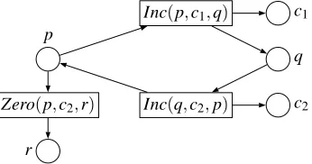
Example 7 Consider the TCM C= (Q,{c1,c2},Ins,p), with Q={p,q,r}and Ins={Inc(p,c1,q), Inc(q,c2,p),Zero(p,c2,r)}. In order to reach a configuration with state r, the first instruction to be executed must be Zero(p,c2,r). Otherwise, the two first executed instructions are Inc(p,c1,q)
and Inc(q,c2,p), so we reach a configuration with c1=c2=1. As there is not a Dec instruction
in this machine, after executing this instructions we cannot reach a configuration with c2=0
anymore, and therefore we cannot reach state r anymore.
We consider only deterministic TCM, that is, TCM such that at each reachable configura-tion there is at most one instrucconfigura-tion that can be executed. Moreover, without loss of generality we assume that if Zero(p,i,q)∈Ins then there is no other instruction of the form Inc(p′,j,q),
Dec(p′,j,q) or Zero(p′,j,q) in Ins, that is, q can only be reached by that instruction (defined as requirement †). Indeed, for each instruction I=Zero(p,i,q)∈Ins we can add two states q1,q2, and replace I by Zero(p,i,q1), Inc(q1,i,q2), Dec(q2,i,q).6 The control-state reachability
problem for deterministic TCM is still undecidable.
Proposition 9 ∀Fcovmodel checking of P/T nets is undecidable.
Proof. We reduce the control-state reachability problem for deterministic TCM to the model
checking problem of a formula in∀Fcov. Let C= (Q,{c1,c2},Ins,q0)be a deterministic TCM
and pend ∈Q. We use the standard simulation of a TCM by means of a P/T net. We define
N= (Q∪ {c1,c2},Ins,F), where:
• F(p,Inc(p,i,q)) =1, F(Inc(p,i,q),q) =1, and
F(Inc(p,i,q),ci) =1 (a token is moved from p to q, and a token is added to ci).
6If we allow instructions that do not modify the counter then it is enough to add a single state q
1and an instruction
p
Inc(p,c1,q)
q
Inc(q,c2,p)
r
Zero(p,c2,r)
c1
c2
Figure 7: Construction of Prop.9for the TCM of Ex.7
• F(p,Dec(p,i,q)) =1, F(Dec(p,i,q),q) =1, and F(ci,Dec(p,i,q)) =1 (a token is moved from p to q, and a token is removed from ci).
• F(p,Zero(p,i,q)) =1 and F(Zero(p,i,q),q) =1 (a token is moved from p to q).
Moreover, F(n,m) =0 elsewhere, and the initial marking of N is{q0}. In N, the number of tokens in cirepresent the value of the counter ciin C. Increasing and decreasing transitions are simulated faithfully. However, the simulation of a transition Zero(p,i,q)can “cheat”, whenever it is fired with tokens in ci. In that case, notice that the marking{ci,q}can be covered. Moreover, because q cannot be reached using a different instruction (requirement (†) above), we know that if such marking is covered then the current simulation has cheated. Focus on Fig. 7, which represents the net built from the TCM of Ex.7. Note that transition Zero(p,c2,r)can be fired even after firing Inc(p,c1,q)and Inc(q,c2,p), when c2is not empty. In this case, this simulation
has cheated.
We considerϕ=F(cov(pend)∨Wm∈Jcov(m)), where J={{ci,q} |Zero(p,i,q)∈Ins}. Notice that all the cheating runs satisfyϕ. We prove that pend can be reached in C if and only if N|=ϕ. For the if part, if C reaches pend then the non-cheating run of N eventually covers pend, so that it satisfiesϕ. Since cheating runs always satisfyϕ, every run of N satisfiesϕ. Conversely, if C does not reach pend then the non-cheating run of N does not satisfyϕ.
5
Conclusions and future work
Table1summarizes the results on model checking of P/T nets, reset nets andν-PNs. In partic-ular, in this work we have proved the undecidability of the fragments LT Lf,L(GF)andL(F) for reset nets andν-PN.
Further study, in order to define more expressive logics for which the model checking problem is decidable, is needed. A possible direction in such study could be the definition of logics with atomic propositions that are more specific of the particular model. Such direction links with the so called Yen’s logics for P/T nets. In the case ofν-PN, the corresponding logic should be able to express properties about the names in the marking.
Language theory was used to prove the difference of expressiveness between reset nets and ν-PNs in [20]. In this sense, it would certainly be interesting to find a logic which distinguishes between reset nets andν-PNs.
Finally, we have proved that the complexity of Fcovmodel checking is non primitive recursive for reset nets and for ν-PN. However, it would be interesting to perform a finer complexity analysis.
Bibliography
[1] M. Ben-Ari, Z. Manna and A. Pnueli. “The Temporal Logic of Branching Time”. Acta Informatica 20, 207-226(1983).
[2] R. Bonnet. “Theory of Well-Structured Transition Systems and Extended Vector-Addition
Systems”. Th`ese de doctorat, Laboratoire Sp´ecification et V´erification, ENS Cachan,
France (2013).
[3] A. Bouajjani and R. Mayr. “Model Checking Lossy Vector Addition Systems”. Interna-tional Symposium on Theoretical Aspects of Computer Science, LNCS vol. 1563, 323-333 (1999).
[4] E. M. Clarke, O. Grumberg, and D. A. Peled. “Model Checking”. MIT Press Cam-bridge(1999).
[5] G. Decker, M. Weske. “Instance Isolation Analysis for Service-Oriented Architectures”. Proceedings of the 2008 IEEE International Conference on Services Computing, 1, 249-256 (2008).
[6] J. Desel and W. Reisig. Place/transition petri nets. Lectures on Petri Nets I: Basic Models, LNCS vol. 1491, pp.122–173. Springer, 1998.
[7] C. Dufourd, A. Finkel, and Ph. Schnoebelen. “Reset Nets Between Decidability and
Unde-cidability”. International Colloquium on Automata Languages and Programming, LNCS
vol. 1443, 103-115 (1998).
[8] J. Esparza and M. Nielsen. “Decidability Issues for Petri Nets”. BRICS Report Series, RS-94-8 (1994).
[9] J. Esparza. “On the decidability of model checking for several µ-calculi and Petri nets”.
Colloquium on Trees in Algebra and Programming, LNCS vol. 787, 115-129 (1994).
[11] K. van Hee, A. Serebrenik, N. Sidorova and M. Voorhoeve. Soundness of
Resource-Constrained Workflow Nets. Applications and Theory of Petri Nets, LNCS vol. 3536,
250-267 (2005)
[12] R. Howell, L. Rosier and H. Yen. “A taxonomy of fairness and temporal logic problems for
Petri nets”. Theoretical Computer Science 82, 341-372 (1991).
[13] P. Janˇcar. “Decidability of a Temporal Logic Problem for Petri Nets.”. Theoretical Com-puter Science 74, 71-93 (1990).
[14] C. Lakos, S. Christensen. A General Systematic Approach to Arc Extensions for Coloured
Petri Nets. Applications and Theory of Petri Nets. LNCS vol. 815, pp. 338-357 (1994)
[15] M. L. Minsky. “Computation: Finite and Infinite Machines” Prentice-Hall (1967).
[16] OASIS Web Services Business Process Execution Language Version 2.0. OASIS Standard (2007).http://docs.oasis-open.org/wsbpel/2.0/wsbpel-v2.0.pdf
[17] A. Pnueli. “The Temporal Semantics of Concurrent Programs” Theoretical Computer Sci-ence, 13, 1-20(1981).
[18] Klaus Reinhardt. “Reachability in Petri Nets with Inhibitor Arcs” Electr. Notes Theor. Comput. Sci. 223: 239-264 (2008).
[19] F. Rosa-Velardo and D. de Frutos-Escrig. Name creation vs. replication in Petri Net sys-tems. Fundamenta Informaticae 88(3). IOS Press (2008) 329-356.
[20] F. Rosa-Velardo and G. Delzanno. “Language-based Comparison of Nets with Black
To-kens, Pure Names and Ordered Data.”. International Conference on Language and
Au-tomata Theory and Applications, LNCS vol. 6031, pp. 524-535. Springer (2010)
[21] F. Rosa-Velardo and D. de Frutos-Escrig. Decidability and Complexity of Petri Nets with
Unordered Data. Theoretical Computer Science 412(34): 4439-4451 (2011)
[22] Ph. Schnoebelen. “Revisiting Ackermann-Hardness for Lossy Counter Machines and Reset