ASSESSING THE POTENTIAL FOR CARBON
SEQUESTRATION IN DEPLETED HEAVY OIL RESERVOIRS
USING ACOUSTIC LOGGING
Mumuni Amadu
[a]and Adango Miadonye
[b]Keywords: carbon sequestration, heavy oil reservoir, heat transfer, acoustic logging, carbon dioxide emission.
As global warming due to anthropogenic greenhouse gases, notably carbon dioxide threatens to take a catastrophic dimension, geological storage of carbon dioxide has been widely accepted as a technically and economically viable remediation strategy. Consequently, targeted geological repositories are saline aquifers, salt caverns, deep unmineable coal seams and depleted oil and gas reservoirs. For storage in depleted oil reservoirs, the stratigraphic trapping capability of overlying low permeability shale is the principal motivating factor for long term containment of anthropogenic gas in oil reservoir until its dissolution and final immobilization by mineral carbonation reactions. Consequently, where the development of the oil reservoir by thermal recovery can lead to thermal pressurization of the cap rock layer, the ability of such a depleted reservoir to contain anthropogenic carbon dioxide must be thoroughly investigated to assess its competency as a proposed geological repository. In this study, seismic theory coupled with that of heat transfer has been used to derive interval velocity for a heavy oil reservoir under thermal recovery. The resulting equation has been validated using published works from literature sources.
* Corresponding Authors
E-Mail: [email protected]
[a] Department of Process Engineering and Applied Science, Dalhousie University, Halifax, NS, Canada
[b] School of Science and Technology, Cape Breton University, P.O. Box 5300, Sydney, NS, Canada.
Introduction
The capture and isolation of anthropogenic carbon dioxide in suitable geologic media have been universally acclaimed as a suitable global warming mitigation step. These geologic repositories could be depleted oil and gas reservoirs, salt caverns, deep unmineable coal seams and deep saline aquifers. In seeking to isolate carbon dioxide in depleted oil and gas reservoirs and deep saline aquifers one fundamental requirement is of technical importance. The reservoir or saline aquifer must be capped by a low permeability geological formation capable of providing long term hydrodynamic trapping mechanism in order to safely contain the injected gas until ultimate dissolution occurs under the subsurface environment. This crucial hydrodynamic trapping mechanism must be effective during injection and post injection periods.1
Among the depleted oil reservoirs are those that were produced using thermal recovery techniques. Where these reservoirs are found at depths capable of sustaining injected carbon dioxide under supercritical conditions such as in China and Venezuela they are possible candidates for carbon geosequestration. However, in view of excessive heating environment connected to their development these deep depleted heavy oil reservoirs need to be thoroughly evaluated for cap rock geomechanical integrity before being included in the inventory of suitable depleted oil reservoirs.2-4 This technical evaluation is necessary because
the high temperature of hot water or steam used in thermal oil recovery methods result in heat transfer from the
reservoir into the overlying cap rocks. The geomechanical implication of this heat transfer is seen in possible thermal pressurization of the resident brine in the cap rock. The low permeability nature of these cap rocks makes it difficult to diffuse excess pore pressure resulting in pore pressure levels exceeding limits required for tensile or shear failure. To obtain an idea about cap rock long term geomechanical integrity there is the need to monitor cap rock performance during thermal operations of deep heavy oil reservoirs. This requires time lapse seismic or acoustic monitoring, which consists of using base line seismic or acoustic survey results as a standard for comparison against current survey results. The aim of this paper is to analytically derive an equation that will link interval velocity to depth temperature during thermal operation designed to produce deep heavy oil reservoirs. Such an equation will enable the calculation of temperature change from acoustic monitoring data where interval velocity versus depth is measured from time to time during thermal operations of deep heavy oil reservoirs.
Theoretical Derivation
The most common approach for linking acoustic interval velocity to pore pressure is the famous Eaton’s empirical equation given as follows:5,8
(1)
Isolating the interval velocity in equation 1 gives:
(2)
i 3p obs obs hyd n V
P P P P
V
1 3 obs p i
obs hyd
P P V V
P P
Assuming a temperature change from initial value T0to T
in the cap rock due to heat transfer from the injected fluid induces a pore pressure change due to aquathermal pressurization the pressure change and temperature change are related by.6
(3)
Integration of equation 3 within appropriate limits gives:
(4)
(5)
(6)
The following quantities will be defined:
(7)
(8)
Equation 2 can be written as:
(9)
Assuming:
(10)
Equation 9 can be written as:
(11)
U is a function of pressure so:
(12)
Differentiating equation 11 with regard to pore pressure gives:
(13)
From equation 10:
(14)
Substituting equation 14 into equation 13 gives:
(15)
(16)
Substituting for dPp from equation 8 into equation 16
gives:
(17)
Substituting for pore pressure from equation 6 into equation 17 gives:
(18)
(19)
13
i p
V P
23
s 0
i pi 1 sf
3
dv T T P dT
s f p w 1 P T c
pip 0 0
P s f T T
p
P T T
w
1
dP dT dT
c
s f w 1 c
p pi 0
PP TT
p 0 pi
P TT P
3 n obs obs hyd V P P P 3 n obs hyd V P P
p
U P1/ 3 i
V U
i i( ( p))
V V U P
2 / 3
i i
p p p
1 3
dV dV dU dU
U
dP dU dP dP
p
dU dP
2 / 32 / 3 i p p 1 3 3 dV U P dP
2 / 32 / 3
i p p
1
3 3
dV U P dP
2 / 31 p s(1 ) sf
3
d P
i 0 0 0 0 02 / 3
i 0 pi
0
2 / 3
i 0 pi
2 / 3 0 pi
2 / 3
i 0 pi 2 / 3
( ) 3 ( ) 3 1 3 1 ( ) 3 V T T T T T T T T T T
dV T T P dT
V T T P dT
dT
T P T
V T T P C
where:
( 0 ); ;
3
A T Ppi BT C (20)
Integration using maple program gives:
(21)
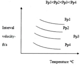
Equation 21 finally links the interval velocity of acoustic wave to temperature. It shows an imminent decrease of velocity with temperature increases in thermal operations related to steam or water injection when temperature in the cap rock changes due to heat transfer from the reservoir.
Interval velocity is a function of depth in the sedimentary basin during well logging. Equation 21 can therefore be written in functional notation as:
(22)
where:
(23)
Z= depth in the sedimentary basin
Derivation of Interval Velocity with Temperature Change
Where there is porosity change as a result of thermal pressurization, the relationship between porosity and transit time or slowness is given by the equation.14
(24)
Transit time or slowness is reciprocal of interval velocity thus observed interval velocity is given by:
(25)
Equation 24 can be written as:
(26)
Differentiating equation 25 with respect to interval velocity gives:
(27)
For pore change resulting from thermal pressurization pore pressure change is related to temperature change as given in equation 3:
(28)
Thus:
(29)
Assuming thermal pressurization of pore fluid results in a deformation that translates into a porosity change this will be given by:7
(30)
From equation 30 the following can be written:
(31)
This implies:
(32)
Equating equation 32 to equation 28 gives:
(33)
This gives the temperature derivative of porosity as:
(34)
obs ma obs ma f ma f ma f ma
t t t t
t t t t t t
i obs 1 V t -1obs ma ma
i
f ma f ma f ma 1
t t t
V
t t t t t t
-2 obs ma
i i f ma f ma
1
t t
d V dV
t t t t
s p s
0
1
0d
C dP
dT
p
s s
0
1
0dP
d
C
dT
dT
sp s 0
1
d
dP
dT
dT
C
ss f
w 0 s
1
1
d
dT
c
C
s
fs 0 s
w
1
1
d
C
dT
c
s f p w 1 dP dT c
0i 2 / 3
( )
( )
C T T V A BT 0
i 2 / 3
(
( ))
( )
(
( ))
C T
T Z
V Z
A BT Z
i
( )
( )
V Z
F Z
Thus:
(35)
The following quantities will be defined:
Equation 35 becomes:
(36)
Integration gives:
(37)
(38)
Thus:
(39)
(40)
Equation 27 gives:
(41)
Substituting for porosity from equation 27 into equation 39 gives:
(42)
Thus:
(43)
This gives the relationship between interval velocity and temperature as:
(44)
In equation 44 the interval transit time for fluid and matrix are constants. All other quantities in the equation on the right hand side are constants except temperature. The equation therefore shows that as temperature increases the denominator increases and the effect is to decrease interval transit time as proven earlier.
Experimental Validation
The experimental validation of this equation requires laboratory measurement of acoustic wave velocity under reservoir conditions where in situ formation stresses are provided in the measuring system. For this paper the experimental validation of the equation will be sought by using experimental results from published literature sources. Equation 18 shows that by using log derived interval velocity the temperature at the given depth can be calculated and this can form the basis of time lapse acoustic monitoring in thermal operations. The parameter A in equation 21 contains pore pressure. Figure 1 shows a theoretical plot of this velocity trend with different pore pressures.
Figure 1. Theoretical plot of Eqn. 22 for different pore pressures
0
0
1
exp
T
T
s 0 s s
f s
w w
1
d
dT
C
C
c
c
f s s
w
0 s s w
C c
C c
d
dT
1
0
01
1
ln
ln
T
T
0 0
1
1
TT
d
dT
0
0
ln T T
obs ma ma
f ma f ma i f ma
1 1
t t t
t t t t V t t
obs ma ma
f ma f ma i f ma
0 0
1 1
1
exp
t t t
t t t t V t t
T T
o o
f ma
mai
t t t T
T
V exp
1
1
0
iT-T 1
ma ma
0 f
1
V
e
t
t
t
Figure 2. The effect of pore pressure on compressional wave velocity at different temperatures9
Figure 3. The effect of pore pressure on shear wave velocity at different temperatures9.
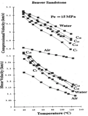
Figure 4. Then effect of temperature on compressional (top) shear (bottom) wave velocities for for different fluid contents Beaver sandstone12
Discussion
The demand for coal (hard coal, brown coal, lignite) has grown by 62 % over the past thirty years. The International Energy Administration (IEA), in its reference scenario, expects coal demand to grow by another 53 % up to 2030 with a possible decline in the market after this period due to carbon constraints in economies (Klaus Brendau).11
This means that anthropogenic emission of carbon is supposed to reflect this growth in energy consumption trend. Since geological sequestration has been accepted by the intergovernmental panel on Climate Change as the most technically feasible mitigating step in reducing global warming, due to anthropogenic carbon dioxide emission, more geological repositories will be required to achieve this environmental remediation objective.
Figure 5. Then effect of temperature on compressional (top) and shear (bottom) wave velocities for different fluid contents of Boise sandstone12
This means that all the target geological repositories, depleted oil and gas reservoirs, salt caverns, deep unmineable coal seams and saline aquifers need to be geologically and technically evaluated for anthropogenic carbon dioxide sequestrations projects on global basis. In line with this objective deep depleted heavy oil reservoirs that have had their cap rocks subjected to excessive heat flow need to be thoroughly evaluated geomechanically during and after thermal operations. This is necessary to ensure that thermal pressurization of resident pore fluid in low permeability geologic formation that has the potential to induce shear and tensile failure did not reduce the hydrodynamic trapping capability of these cap rocks by impacting their capillary entry pressures and their required low permeabilities.
To be able to carry out this assessment there is the need to be able to obtain information about the heat transfer characteristic of the cap rock and the temperature evolution during thermal operation. Two approaches are possible. One an indirect method and it is based on the mathematical modelling of heat transfer in the cap rock reservoir system and solution of the temperature evolution for both reservoir and cap rock. In the hydrogeological industry this approach has been used to obtain the temperature field of the system in matters related to aquifer thermal energy storage for seasonal exploitation. In this paper an alternative approach base on a direct method of the time lapse acoustic monitoring of deep heavy oil reservoir thermal exploitation is proposed. This has to do with the time to time measurement of a seismic attribute which is the interval velocity. To be able to achieve this objective an equation that links interval velocity to temperature change has been presented. Since acoustic data such as interval velocity is depth related the corresponding temperature will be the temperature at the depth following thermal operation. The difference between this and the initial temperature imposed by the local geothermal gradient will be the temperature change since thermal operation began. Due to lack of laboratory resource experimental validation of the equation was not possible but interpretation of the equation by comparison with experimental data and graphical plots from literature sources shows that the equation is capable of predicting similar experimentally determined trends. In this regard, Figures 2 to 6 indicate a decrease in interval velocity for primary and shear waves with temperature increase which has been theoretically established by this work.
Application to thermal monitoring of critical interval velocity
Time lapse seismic or acoustic monitoring involves the time to time measurement of seismic or acoustic attributes of the earth related to saturation change resulting from fluid injection, change in bulk density resulting from hydraulic fracturing, change in interval velocity resulting from temperature change accompanying heat injection etc. and comparing these surveys with a base line survey acquired before any operations began. For a cap rock submitted to heat accumulation due to heat transfer from an injected fluid, the critical temperature resulting in tensile failure due to thermal pressurization of pore fluid will result in a critical interval velocity as given by equation 22:
The temperature at which this occurs is given by substituting critical temperature for temperature in equation 22. This temperature will be a function of depth as predicted by equation 22.
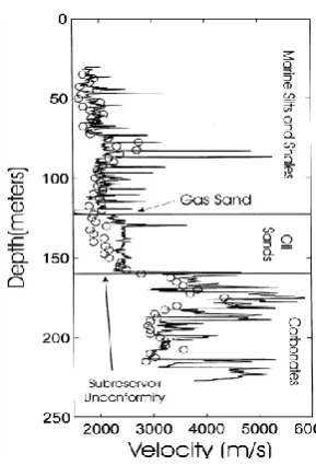
Figure 7 gives the observed sonic log velocities versus travel time (a) prior to heating as against hypothetical sonic log velocities (b) after heating of the reservoir. The figure shows that prior to heating the average elastic wave velocity between 120 and 150 meters was about 2400 m/s. After heating the average elastic wave velocity over the same
Figure 7. Comparison of logging data before and after heating10
Figure 8. Sonic log showing characteristic interval velocity (line and open interval velocity after thermal recovery open (circle)10
i
i 2
3 C T T Z
V Z F Z
A BT Z
depth interval is seen to be about 2100 m/s (Figure 7(b) and (c)). The figure clearly shows a shift of the interval velocity after thermal recovery to the left, a clear evidence of decrease in interval velocity after thermal operations. This shows that by using log derived data such as the interval velocity the temperature of the cap rock interval corresponding to these time lapse acoustic log can be deduced using relevant thermophysical parameters together with the equation 22.
Figure 8 also shows a graphical plot of sonic log characteristic interval velocity of a heavy oil reservoir (line) consisting of sand and with an overlying marine silt and clay cap rock and the characteristic interval velocity after thermal recovery. It clearly shows a shift of the interval velocity after thermal recovery to the right in both the reservoir and the cap rock, a clear evidence of decrease in interval velocity after thermal recovery of heavy oil. This shows that by suing log derived data such as the interval velocity the temperature of the cap rock interval corresponding to these time lapse acoustic log can be deduced using relevant thermophysical parameters together with equation presented by this work.
Application to Thermal monitoring of Critical State Properties
Monitoring of subsurface operations refers to the systematic measurements and detection of subsurface property changes in response to subsurface related processes such as temperature and stress changes. These are invariably related to thermal operations in tertiary enhanced oil recovery of heavy oils or the injection of fluid into petroleum reservoirs as encountered in secondary oil recovery and carbon dioxide injection into saline aquifers. Each of these activities has the potential to perturb subsurface pressure and temperature regimes. In either of these operations there are two types of monitoring objectives.13 Deep monitoring of the reservoir or geologic
repository integrity and most importantly plume evolution for the case of carbon geosequestration and near surface monitoring is designed to ensure public safety and environmental health. These two principal aims underlie traditional monitoring operations of subsurface operations but in the case of carbon geosequestration where cap rock (low permeability overlying) formation with hydrodynamic trapping capability is fundamental to long term safe geological isolation of the gas, monitoring of this formation deserves to be considered and is the key focus of this work. In this regard, while thermal and fluid injection operations change the pressure and temperature regimes of the reservoir and therefore stress regimes, these two operations will not cause flow in the cap rock but will induce similar stress changes through heat transfer and pressure build up in the reservoir particularly in the vicinity of the injection wells. Heat transfer from the injected fluid into the cap rock causes thermal loading of the resident fluid with attendant excess pore pressure build ups while fluid pressure at the base of the cap rock induces bending in the cap rock with attendant stress problems. To assess the potential of the cap rock for carbon sequestration, therefore, requires monitoring the cap rock and making sure critical pressures and stresses are not exceeded to cause failure and undermined the geomechanical integrity.
Conclusion
Global warming due to anthropogenic emission of carbon dioxide has reached unprecedented levels. To mitigate global warming effects due to this gas geological storage of anthropogenic carbon dioxide is the most technically feasible and affordable solution from both immediate and long term planning perspectives. To achieve this, depleted oil reservoirs are good candidates for geologic repositories. Among these reservoirs there those that containing oils that cannot be produced without heat inputs. These are deep heavy oil reservoirs where carbon dioxide can exist under supercritical conditions. The occurrence of these reservoirs has been reported in China where anthropogenic carbon dioxide emissions are at record levels. The implication is that the excessive heat inputs can render the cap rocks of these reservoirs geomechanically unsuitable for carbon sequestration purposes. To be able to determine their suitability therefore requires monitoring their thermal operations. One way to do this is to use time lapse seismic or acoustic monitoring. It consists of measuring seismic attributes such as velocity or acoustic impedance from time to time and a comparison of this with base line survey results.
To be able to achieve this objective this paper has presented an equation that links interval velocity to temperature during thermal operation designed for heavy oil exploitation. Although lack of acoustic logging data for such purposes are not available for testing the equation the observation is that it theoretically predicts experimental trends reported in literature works and can be used to aid temperature computations using acoustic logging data and inputs of petrophysical and thermophysical property data.
Greek Symbols and Nomenclatures
Pp=Pore pressure, psi
Pobs=Overburden pressure, psi
Phyd=Hydrostatic pressure, psi
Vi= Interval velocity, ft s-1
Vn= Normally compacted shale interval velocity, ft/s
Φ = porosity change,
Φ0 = initial porosity,
Cs = grain compressibility,
Pp = pore pressure
References
1Durk-Jan Peet (Editor):” Geotechnology and Sustainable
Development: Challenges for the Ffuture” 2008, ISBN 978-90-5972-293-4
2Liu Wenzhang Research Institute of Petroleum Exploration and
Development, CNPC, China:” Thermal Recovery Status and Development Prospect for Heavy Oil in China” UNITAR Centre for Heavy Crude and Tar Sands. No.198, 1998
3Head, I. M., Jones, D. M. and Larter, S. R., Nature, 2003, 426(20),
4Eremenko, E., Kochanova, S., Kourenko, M., Perevozchikov,
S., ”Simulation of a Sector Model of the Heavy Oil Thermal Recovery” Society of Petroleum Engineers, 2004.
5Eaton, B. A., World Oil, 1972, 182, 51-56.
6Shi, Y.-L. and Wang, C.-Y., J. Geophys. Res., 1986, 91(B2),
2153-2162.
7Ghabezloo, S. and Sulem, J., Ital. Geotechn. J., 2012, 1, 29-43. 8Chopra, S. and Huffman, A., “Velocity determination for pore
pressure prediction” 28 CSEG RECORDER, April 2006
9Setyowiyoto, J. and Samsuri, A., Int. J. Eng. Technol., IJET, 2009,
9(10), 80-93.
10Schmitt, D. R., Geophysics, 1999, 64(2), 368–377.
11Klaus Brendow, “World Coal Perspectives to 2030” World
Energy Council, Geneva/London, 2004.
12Wang, Z. and Nur, A, Geophysics, 1990, 55(10), 723-733. 13Wielopolski, L., Int. J. Environ. Res. Public Health, 2011, 8,
818-829.
14Raymer, L. L, Hunt, E. R., and Gardner, J., S., An Improved
Sonic Transit Time-to-Porosity Transform”, SPWLA Twenty-First Annual Logging Symposium, July, 8-11,1980.