The analysis and advanced extensions of canonical correlation analysis

(1)

The Analysis and Advanced Extensions of Canonical Correlation

Analysis

Daniel V. Samarov

A dissertation submitted to the faculty of the University of North Carolina at Chapel Hill in partial fulfillment of the requirements for the degree of Doctor of Philosophy in the Department of Statistics and Operations Research.

Chapel Hill 2009

Approved by

Advisor: Dr. J. S. Marron

Co-Advisor: Dr. Yufeng Liu

Co-Advisor: Dr. Alexander Tropsha

Reader: Dr. Perry Haaland

(2)

(3)

ABSTRACT

DANIEL V. SAMAROV: The Analysis and Advanced Extensions of Canonical Correlation Analysis

(Under the direction of J. S. Marron, Yufeng Liu and Alexander Tropsha)

Drug discovery is the process of identifying compounds which have potentially mean-ingful biological activity. A problem that arises is that the number of compounds to search over can be quite large, sometimes numbering in the millions, making experimen-tal testing intractable. For this reason computational methods are employed to filter out those compounds which do not exhibit strong biological activity. This filtering step, also called virtual screening reduces the search space, allowing for the remaining compounds to be experimentally tested.

In this dissertation I will provide an approach to the problem of virtual screening based on Canonical Correlation Analysis (CCA) and several extensions which use kernel and spectral learning ideas. Specifically these methods will be applied to the protein-ligand matching problem.

(4)

LIST OF FIGURES

1.1 Toy example data. The points highlighted in red correspond to the protein ligand pair 11gs, and the points connected to it by dashed black lines are its

three nearest neighbors in each space. The observations highlighted cyan

are neighbors in both spaces, and those highlighted in blue and purple are

neighbors only in the protein, and ligand spaces respectively. The green

point Lnew in the ligand space corresponds to a simple weighted average of

the cyan points and the purple point; i.e. of the nearest neighbors of 11gs

in the protein space. . . . 6 1.2 Four bivariate toy data sets, with differing correlation. The top plots

cor-respond to the scatterplot view of data and the bottom plots are connectivity

plots of the data. The blue points, on the bottom set of plots, are the x

coordinate values and the red points are the corresponding y coordinate values. In the top set of plots as correlation increases points begin falling

closer to the 45 degree line. In the bottom set of plots the dashed green

lines become increasingly parallel to each other. . . . 8 1.3 An illustration of the relationship between correlation and angle between

two vectors. Note that we assume that the vectors have been mean centered. 9 1.4 The direction vectors and the projected value of each point. The top row

of plots shows the first direction vector, in red, and the projections onto

it. The bottom row of plots show the second direction vector, in green, and

(8)

1.5 Projection of the data in Figure 1.1 onto the first and second canonical vectors. In contrast to Figure 1.1 the point 11gs now shares the same

neighbors in both spaces and the predicted value in green is much closer to

the actual value.. . . 11 1.6 The plots in the upper right half of the figure are the projections of the

RLP800 receptor training data onto their first four principal components.

The plots along the diagonal show the distribution of the projected values

with the red curve being a kernel density estimate of the projections and

the percentage in the upper right hand corner the proportion of variation

explained by that principal component. The plot on the lower left side

show the eigenvalues of all 150 principal components. The red curve is the

cumulative sum of the eigenvalues. . . . 18 1.7 Same layout as in Figure 1.6. but for the RLP800 ligand training data. . 19

2.1 Four groups of four plots, each group consists of a plot of the X and Y raw data spaces (top left and right) and the projections of these spaces onto

their respective first and second canonical directions (bottom left and right).

Group (a) shows the data with no transformation. All subsequent groups

have been transformed. In group (b) The data in the X space have been

rotated 30◦ _{counterclockwise and in the Y space the data have been rotated}

75◦ _{clockwise. In group (c) the points in the X space have been scaled by}

5

3 and in the space Y by 2

3. In group (d) the means of the points have been

shifted such that the centers are now at ₋3₄,1₂and 3₄,₋1₄. The point of all these illustrations is that in all four groups of plots the bottom left and

right plots, the projections into the canonical correlation space, are all the

(9)

2.2 A simulated example of the canonical vectors in X space in the presence of strong multicollinearity between the first and third descriptors. The major

issue here is the large amount of variation in the canonical directions from

one sample to the next despite the fact that the data are drawn from the

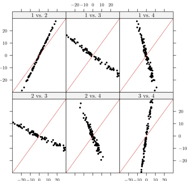
same distribution. . . . 41 2.3 Plot of the projected values of a new set of observations onto the canonical

direction vectors shown in Figure 2.2. Each panel shows the plot of one

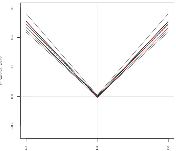
projection versus another (only four projections are shown). . . . 42 2.4 This is a plot of the canonical direction vectors found from RCCA. The

dashed red line is the theoretical direction. In contrast to the direction

found by linear CCA the directions found by regularized CCA display little

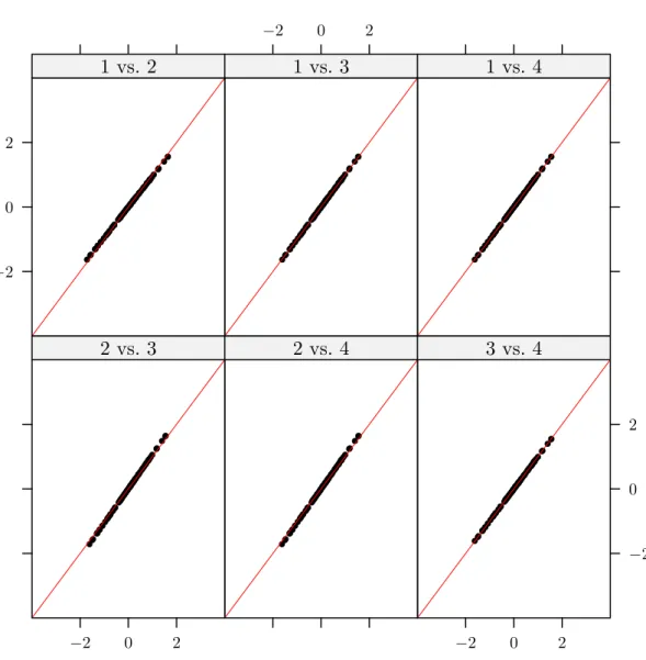
variation from one sample to the next and lie near the theoretical direction. 43 2.5 A plot of each pair of projected values of the new data onto each of the

direction vectors shown in Figure 2.4 against one another. As can be seen

the projections are all quite similar to one another, in contrast to standard

CCA where there was a great deal of variation from one set of directions

to the next. . . . 44 2.6 New toy example data. The points highlighted in red correspond to the

protein ligand pair 1a1e, and the points connected to it by dashed black lines

are its three nearest neighbors in each space. The observations highlighted

in blue and purple are neighbors only in the protein and ligand spaces

respectively. The green point Lnew in the ligand space corresponds to a

simple weighted average of the cyan point and the purple points, i.e. of the

(10)

2.7 These plots depict the same data as in Figure 2.6 with points highlighted according to whether they appear in the same cluster in both spaces. For

example, consider the green points, these observations appear in the same

cluster in both protein and ligand space. The data has been generated such

that points that appear in the same cluster in both spaces are highly correlated. 46 2.8 The linear CCA direction vectors and the projected value of each point

colored as in Figure 2.7. On the first row of plots the first two panels

show the first direction vector and the projections onto it in protein and

ligand space respectively. The last panel on the top row of plots is a plot

of the first canonical variate in protein space against the first canonical

vector in ligand space. If the directions we found were able to capture the

underlying relationship between the two spaces we would expect these points

to fall along the 45◦ _{line. The second row of plots shows the same set of} plots as the top row of plots but for the second canonical direction. A visual

assessment of the projected values of the observations in each space shows

how different the distribution of points is along the canonical vectors. This

discrepancy is further highlighted by noting how different the location of

the colored points are along the canonical vectors. The implication of this

is that the correlation, i.e. alignment is not very good as reflected by the

canonical correlations of 0.46 and 0.34. . . . 47 2.9 CCA Projected space. In contrast to Figure 1.4, linear CCA appears to

have made the prediction worse. . . . 48 2.10 A plot of the canonical correlations from the RLP800 data set with the

training data shown in black and the test data shown in red. From a visual

assessment of the data it appears as though the two spaces are fairly well

(11)

2.11 On the left are plots of the first three canonical variates in protein and lig-and space respectively. The red curves are the associated density estimates

of the canonical variates. This is meant to provide some insight into the

distribution of the data within a space as well as how well aligned points

are between spaces. On the right is a plot of the canonical correlations

associated with each of the 150 canonical vectors. . . . 49 2.12 Similar to Figure 2.10 but with one of the test points highlighted as well as

its three nearest neighbors. The color scheme is similar to that of the toy

examples discussed earlier this section. . . . 50 2.13 A histogram showing the ranks resulting from prediction on the test data

from the RLP800 dataset. The vertical red line indicates the average rank

(approximately 10) using CCA and the vertical green line the method

im-plemented in Oloff et al. (2006) (approximately 18). . . . 51 2.14 Similar to the histogram above but using the WDI data. The mean rank

using CCA is approximately 67 while the previous method yielded a mean

result of approximately 310 . . . 52

3.1 A plot of the data generated such that the underlying relationship between points is non-linear. The observation highlighted in red, 1a94, is the new

observations which we are trying to predict. The points joined to it by

dashed black lines are its nearest neighbors. The points highlighted in cyan

correspond to a point which is a nearest neighbor of 1a94 in both spaces.

Points highlighted in blue and purple correspond to points which are only

neighbors in either protein or ligand space respectively. The point labeled

Lnew _{in ligand space corresponds to a simple average of the points 1a08,}

(12)

3.2 A plot of the data projected onto the first two canonical vectors in both protein and ligand spaces. The directions found by standard CCA do not

provide a good alignment between the two spaces.. . . 56 3.3 A plot of the protein data in kernel space. The color scheme is the same

as in Figure 3.1. Looking at Figure 3.4 the overall correspondence between

points in protein space and ligand space is much better than in the original

(object) space. . . . 57 3.4 A plot of the ligand data in kernel space. The color scheme is the same

as in Figure 3.1. As discussed in Figure 3.3 the correspondence between

points in ligand and protein space is much better than in the original object

space. This improved mapping will allow CCA to do a better job aligning

the two spaces. . . . 58 3.5 This is a plot of the projection of the data in protein feature space onto

the first, second and third canonical vectors. As can be seen not only

does the new observation 1a94 (red) have the same 3 nearest neighbors in

both protein and ligand space but the prediction of the new ligand, Lnew

highlighted in green below in Figure 3.6 is close to the actual value of 1a94. 59 3.6 See Figure 3.5 for details. . . . 60 3.7 A toy example illustrating the cases when the distribution of points within

a space is non-standard and heterogeneous. . . . 72 3.8 These plots highlight how the distribution of points in one space is related

to the distribution of points in the other. Looking at the plots on the left in

Figure 3.8 each of the three clusters is in fact composed of two subclusters.

Likewise each of the two clusters in the plots on the right are composed of

three subclusters. . . . 73 3.9 In this plot each of the six underlying subgroups shown in Figure 3.8 is

(13)

3.10 Scatterplot matrix of the first five KCCA direction vectors for the data shown in Figure 3.7. Each of the colors in this plot corresponds to one of

the six underlying subpopulation in the data (see Figure 3.8 for details). . 74 3.11 On the left are plots of the first three canonical variates in protein and

lig-and space respectively. The red curves are the associated density estimates

of the canonical variates. This is meant to provide some insight into the

distribution of the data within a space as well as how well aligned points

are between spaces. On the right is a plot of the canonical correlations

associated with each of the 637 canonical vectors. . . . 75 3.12 A plot of the kernel canonical correlations from the RLP800 data set with

the training data shown in black and the test data shown in red. From a

visual assessment of the data it appears as though the two spaces are fairly

well aligned. . . . 76 3.13 Similar to Figure 3.12 but with one of the test points highlighted and only

its three nearest neighbors. The color scheme is similar to that of the

previous toy examples discussed in the linear case. . . . 77 3.14 A histogram showing the large improvement in rank resulting from KCCA

prediction on the test data from the RLP800 dataset. The vertical red line

indicates the average rank (approximately 7.1) using KCCA, the blue line

shows the average rank using CCA (approximately 10) and the vertical

green line the method implemented in Oloff et al. (2006) (approximately 18.1). . . . 78 3.15 Similar to the histogram above but using the WDI data. The mean rank

using KCCA is approximately 56, RCCA is approximately 67 and the

(14)

4.1 A plot of the data as described in Scenario 1. In the Label Space plot the means are connected by a dashed black line, the corresponding distance

between the means is ∆ = _||µ+−µ−||. The solid circles and lines corre-spond to the support type and radius of the support, respectively of the two

groups (“+” in red and “₋” in green). The dashed circles and connecting lines indicate the2r-neighborhoods of the two points in each group that are closest to the other group. . . . 106 4.2 Continuation from the example in Section 3.7. This is a scatterplot matrix

of the projections onto the first five IKCCA directions using the kernel in

(4.15). Unlike the projections shown in Figure 3.10 here we are able to

separate out the six groups.. . . 117 4.3 A plot of the first four indefinite kernel canonical direction vectors in the

smiley face space from the example in Section 3.7 using the kernel in

(4.15). These plots allow us to visualize how the canonical vectors

sep-arate out each of the clusters. . . . 118 4.4 A plot of the first four indefinite kernel canonical directions vectors in the

cluster space from the example in Section 3.7 using the kernel in (4.15). . 118 4.5 The RLP 800 data set. The red line corresponds to IKCCA, the orange

line corresponds to KCCA, the blue line corresponds to CCA and the green

line corresponds to the method from Oloff et al. (2006). . . . 119 4.6 The WDI data set. The red line corresponds to our method using IKCCA,

the orange line corresponds to KCCA, the blue line corresponds to CCA

(15)

CHAPTER 1

Introduction

Recent advances in biology, genetics and chemistry have led to an influx in the amount of information available on a wide variety of biological processes. A major issue facing scientists is finding meaningful ways of utilizing this data to better understand the mech-anisms of the diseases that affect humans. A key element in dealing with the challenges involved in understanding and analyzing this type of information and the unique prob-lems associated with them is the development of new statistical methodology.

Of interest to scientists is using the many different ways of measuring or viewing the same (or similar) biological, genetic or chemical process in order to better understand the key elements driving them. Consider the following example:

In the field of cheminformatics, drug discovery is a key step in the process of iden-tifying compounds which may have potentially meaningful biological activity as related to a particular disease process. The process of drug discovery typically begins with the identification of a new or existing drug target, typically these targets are proteins. Pro-teins are large organic compounds composed of amino acids and are the building blocks from which all cells are built and are responsible for almost all cell function. The two predominant families of target proteins in drug discovery are G-protein-coupled receptors (GPCR) and protein kinases. About half of all known drugs work through GPCR’s.

(16)

transmembrane receptors bind extracellular signaling molecules, called ligands. Ligands include other proteins and small peptides (short sequences of amino acids), as well as derivatives of amino acids and fatty acids. Once bound these signaling molecules set off a chain of intracellular signaling events. These signaling events are generally mediated by protein kinases and lead to the alteration of some target proteins ultimately leading to a change in cell behavior.

The reason GPCR’s and protein kinases are so important is that in both normal and abnormal cell activity, they are used as lines of communication. In the event of abnormal cell activity they are natural control points.

Consider the case where the target is a novel GPCR, ligands are then screened for their ability to inhibit or stimulate that GPCR. A problem that arises is that the number of compounds to search over can be quite large, sometimes numbering in the millions. Subsequently, experimental verification of protein-ligand interaction can be extremely time consuming and costly or in some cases simply not possible due to time and/or cost constraints. For this reason computational methods are employed to filter out those compounds that do not exhibit a strong relationship with a given receptor. This filtering step reduces the search space allowing for the remaining compounds to be experimentally tested.

(17)

the number of descriptive variables typically ranging from 150 to as many as 800 or more. The prediction problem can be generally stated as follows: for a set of n known protein ligand pairs, with dX and dY descriptors, given a new protein we want to be

able to predict what ligand will bind to it. Let xi _∈ RdX and yi ∈ _RdY, i = 1, . . . , n

denote a protein ligand pair. The sample of pairs is collected in matricesX_∈Rn×dX and Y _∈Rn×dY _with _xi _and _yi _{as the descriptors for a row.}

Our approach to this problem is based on the structural relationship between these molecules. Specifically, that there is a strong (complementary) relationship in the stere-ochemical layout (the relative spatial arrangement of atoms within a molecule) between the protein and its ligand(s). Thus, if we can find a way to align the space of proteins and ligands, then we may be able to exploit this structural relationship to predict which pairs match up.

1.1 General Framework

Casting the protein-ligand matching problem into a general framework, following the discussion of Bach and Jordan (2002) and Fukumizu et al. (2007), our example consists of two multivariate random variables X and Y belonging to Rd_{. In the context of our}

example these random variables correspond, respectively, to proteins and ligands. Lets and ligands. Let fX ∈ HX and fY ∈ HY be mappings from RdX and RdY to R, where HX and HY are spaces of functions. The type of functions we consider are, for example,

bilinear maps, fX(X) = hX,wXi and fY(Y) = hY,wYi. Define S : R×R → R to be

a function measuring the similarity between two random variables. An example of a similarity measure is Pearson correlation. It is important to note that the notation _S is defined here in terms of the population random variables X and Y, as opposed to their sample counterparts. When referring to the sample, i.e. empirical similarity measure we will write _Sb(so for example we would write corr for sample correlation)._d

(18)

similar-ity between proteins and ligands is maximized, this leads to the following optimization problem

ρ_H = max

fX∈HX,fY∈HY S

(fX(X), fY(Y)) (1.1)

where the subscript_H = (_HX,HY) denotes the spaces of functions over which the

simi-larity is being maximized.

The selection of a meaningful measure of similarity is context dependent. All similar-ity measures have relevance in certain circumstances. Examples of similarsimilar-ity measures include correlation, covariance, and mutual information. The one which we will focus on is correlation.

Defining _HX and HY to be the Hilbert spaces of bilinear maps taking the form

fX(X) =hX,wXiandfY(Y) =hY,wYirespectively, the problem as stated in (1.1) then

becomes the well known Canonical Correlation Analysis (CCA) (Hotelling (1936)). The optimization problem in (1.1) then takes the form

ρ_H= max wX,wY

corr(_hX,wX_i,_hY,wY_i) = max wX,wY

cov(_hX,wX_i,_hY,wY_i)

p

var(_hX,wX_i)pvar(_hY,wY_i) (1.2)

The general framework of (1.1) will allow for a natural extension of linear CCA to kernel CCA (KCCA) by defining_HX andHY to be reproducing kernel Hilbert spaces (RKHS).

This will be discussed in further detail in Chapter 3. CCA has a number of appealing properties, including

1. Extensions to kernel based methods, (i.e. Kernel CCA (KCCA)), discussed in Kuss and Graepel (2003), Hardoon et al. (2004) and Bach and Jordan (2002).

(19)

data is known to be normally distributed this can be shown directly. A connection between MI and KCCA is discussed in Bach and Jordan (2002).

4. An extension of CCA to more than two data sets is presented in Kettenring (1971).

5. Connection to linear discriminant analysis (LDA) (Bie (2005) and Hastie et al.

(1995))

An illustration of the protein-ligand matching problem may help in the understanding of CCA and its application to this problem as well as its extension to other similar problems.

1.2 Two Space Toy Example

Consider the protein-ligand matching problem as outlined above. For this toy example we set n = 10 and d = 2. Suppose the descriptors for this toy example are Molecular Weight (MW) and Surface Area (SA) of the molecule. Recall that each row of X(10×2)

and each row ofY(10×2) corresponds to an observation, a protein or a ligand respectively,

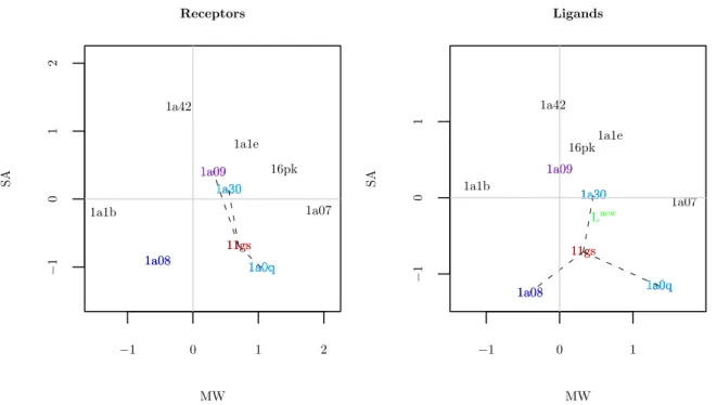
and the columns correspond to the descriptors MW and SA. The pairs are identified by a unique label, corresponding to ID’s from the Protein Data Bank (PDB) (www.pdb.org). Figure 1.1 shows the two toy data sets.

From Figure 1.1 it can be seen that the distribution of points in the two spaces are quite similar in the sense that the location of corresponding points in the two spaces are close. The points connected to 11gs (red) by dashed black lines are its three nearest neighbors. The cyan points are neighbors shared in both spaces and the blue and purple points are mismatched. Two of three neighbors are shared in common (in the Euclidean sense).

(20)

−1 0 1 2

−1

0

1

2

Receptors

MW

SA

11gs 16pk

1a07

1a08

1a09

1a0q 1a1b

1a1e

1a30 1a42

11gs

1a30

1a08 _1a0q_1a0q

1a30 1a09

1a0q 1a30

−1 0 1

−1

0

1

Ligands

MW

SA

11gs 16pk

1a07

1a08 1a09

1a0q 1a1b

1a1e

1a30 1a42

11gs

1a0q 1a30

1a09

1a30

1a08 1a0q1a0q

1a30

Lnew

Figure 1.1: Toy example data. The points highlighted in red correspond to the protein ligand pair 11gs, and the points connected to it by dashed black lines are its three nearest neighbors in each space. The observations highlighted cyan are neighbors in both spaces, and those highlighted in blue and purple are neighbors only in the protein, and ligand spaces respectively. The green point Lnew in the ligand space corresponds to a simple weighted average of the cyan points and the purple point; i.e. of the nearest neighbors of 11gs in the protein space.

and purple in ligand space) would yield a relatively poor prediction despite the strong apparent similarity between the two distributions of points. This dissertation studies more sophisticated approaches to exploiting this similarity.

In Section 1.1 the idea of similarity between two distributions was introduced. In our current example the type of similarity measure that is needed is one that tells us how well aligned the two spaces are. The functions fX and fY we consider will be ones

which place appropriate weights on the features (i.e. descriptors) that best align the two distributions.

(21)

sets, each consisting of two spaces, X and Y with dX = dY = 1 at different levels of

correlation. For each data set two quite different views are considered. The top row of plots are conventional scatterplots of the data and the bottom set of plots areconnectivity plots which provide a different view of the association between pairs of points. In the connectivity plots points are shown as the (green) segments connecting thex-coordinates (blue points) and y-coordinates (red points). This view highlights the similarity of the pairs.

As correlation increases (moving from the left panels to the right) the difference between the values of the points in the X and Y space becomes smaller. This is reflected in the top set of plots in Figure 1.2 as the observations tend to fall closer to the 45 degree line in the right hand panels. In the bottom set of plots the dashed green lines become increasingly parallel to each other. Based on these observations maximizing the correlation between the sets of points x and y is equivalent to maximizing their coordinate-wise alignment.

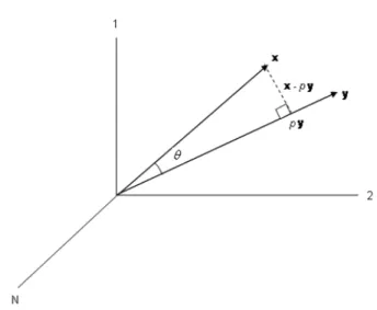
Yet another way to interpret correlation is as the cosine of the angle between the vectorsx and y(Anderson (2003)), assuming they are mean centered. This relationship is easy to verify. Using the idea of projections provides concreteness to the interpretation of correlation as a measure of alignment. Define the projection coefficient p to be the scalar such that the vectorpy is orthogonal to x₋py; solving the following for p

0 =pyT(x₋py) = p(yTx₋pyTy),

we have that, p = yT_x_/_yT_y_{. Next decompose} _x _as _x _{= (}_x

−py) +py, see Figure 1.3. The absolute value of the cosine of the angle betweenx and y is the same as the length of py divided by the length of x;

(22)

−0.4 −0.2 0.0 0.2 0.4

−0.4

0.0

0.4

Correlation = 0

X space

Y space

−0.4 −0.2 0.0 0.2 0.4

0.0

0.5

Correlation = 0.5

X space

Y space

−0.4 −0.2 0.0 0.2 0.4

−0.2

0.2

0.4

Correlation = 0.9

X space

Y space

−0.4 −0.2 0.0 0.2 0.4

−0.4

0.0

0.2

0.4

Correlation = 0.99

X space

Y space

−0.4 −0.2 0.0 0.2 0.4

−0.4

0.0

0.4

Correlation = 0

X space

Y space

−0.4 −0.2 0.0 0.2 0.4

0.0

0.5

Correlation = 0.5

X space

Y space

−0.4 −0.2 0.0 0.2 0.4

−0.2

0.2

0.4

Correlation = 0.9

X space

Y space

−0.4 −0.2 0.0 0.2 0.4

−0.4

0.0

0.2

0.4

Correlation = 0.99

X space

Y space

Figure 1.2: Four bivariate toy data sets, with differing correlation. The top plots corre-spond to the scatterplot view of data and the bottom plots are connectivity plots of the data. The blue points, on the bottom set of plots, are the x coordinate values and the red points are the corresponding y coordinate values. In the top set of plots as correlation increases points begin falling closer to the 45 degree line. In the bottom set of plots the dashed green lines become increasingly parallel to each other.

So in terms of (1.2) above, maximizing the correlation between xand yis equivalent to minimizing the angle between them. As the angle goes to zero the closer each pair of coordinates in both n vectors becomes (modulo a scale factor). This can be seen in Figure 1.3 as the angle goes to zerox₋py goes to zero.

(23)

Figure 1.3: An illustration of the relationship between correlation and angle between two vectors. Note that we assume that the vectors have been mean centered.

Figure 1.5 shows the projections of the data onto the first two canonical vectors (note that separate directions are found in protein and ligand space). We can see that with the slight modification in alignment that has resulted from the CCA projections, the point 11gs now shares the same neighbors in both spaces. In particular note that now the predicted value in the projected ligand space is much closer to the actual value (again using the simple average).

This is a simplified example and in most cases the relationship between points in different spaces may be far more complicated. In coming sections we begin with the simplest case scenario, i.e. standard CCA and related methods. This is used as a start-ing point to motivate and develop methodology and theory appropriate for increasstart-ingly complex problems. Along the way we address the strong and weak points of these various methods.

1.3 Benchmark Data Sets

(24)

−1 0 1 2

−1

0

1

Receptors

MW

SA

11gs 16pk

1a07

1a08 1a09

1a0q 1a1b

1a1e

1a30 1a42

−1 0 1 2

−1

0

1

Ligands

MW

SA

11gs 16pk

1a07

1a08 1a09

1a0q 1a1b

1a1e

1a30 1a42

−1 0 1 2

−1

0

1

Receptors

MW

SA

11gs 16pk

1a07

1a08 1a09

1a0q 1a1b

1a1e

1a30 1a42

−1 0 1 2

−1

0

1

Ligands

MW

SA

11gs 16pk

1a07

1a08 1a09

1a0q 1a1b

1a1e

1a30 1a42

Figure 1.4: The direction vectors and the projected value of each point. The top row of plots shows the first direction vector, in red, and the projections onto it. The bottom row of plots show the second direction vector, in green, and the projection onto it.

1. A set of 800 chemically, and functionally diverse protein-ligand pairs obtained from the PDBbind Database (Wang et al. (2004)). These compounds are described by a set of 150 descriptors. We will refer to this data set as the RLP800 data.

(25)

−0.5 0.0 0.5

−0.5

0.0

0.5

Receptors

First Canonical Direction

Second Canonical Direction

11gs 16pk

1a07

1a08 1a09

1a0q 1a1b

1a1e 1a30 1a42

11gs 1a30

1a08

1a0q

1a0q 1a30

1a08

1a0q 1a30

1a08

−0.5 0.0 0.5

−0.5

0.0

0.5

Ligands

First Canonical Direction

Second Canonical Direction

11gs 16pk

1a07

1a08 1a09

1a0q 1a1b

1a1e 1a30 1a42

11gs

1a0q 1a30

1a08

1a30

1a08

1a0q

1a0q 1a30

1a08

Lnew

Figure 1.5: Projection of the data in Figure 1.1 onto the first and second canonical vectors. In contrast to Figure 1.1 the point 11gs now shares the same neighbors in both spaces and the predicted value in green is much closer to the actual value.

1.3.1 Ligand Prediction

Recall the example discussed in Section 1.2. In that example we first used CCA to define a mapping between the space of receptors and the space of ligands by projecting onto the first pX ≤ dX and pY ≤dY directions (Figures 1.4 and 1.5). Let us define the

projected values of the observations in X and Y space onto their firstpX andpY canonical

vectors as

xwi,p = w1X, . . . ,w pX X

T

, xi _∈RpX_, _i_{= 1, . . . , n} yw

i,p = w1Y, . . . ,w pY Y

T

, yi _∈RpY_, _i_{= 1, . . . , n}

The sample of pairs are collected in matrices Xw

p ∈ Rn×pX and Ypw ∈ Rn×pY with xwi,p

and yw

(26)

The method of prediction and assessment of model performance used, in the context of the protein-ligand matching problem, has similarities and differences with more tra-ditional statistical definitions of these concepts. Prediction in this problem is similar to traditional definitions in the following sense: given a new input, xnew, and it’s projection onto the first pX canonical vectors in X space (call this projected value xwnew,p), we want

to predict the value of its unobserved pair, yw

new,p, in canonical correlation space.

There is an important distinction to draw here. Traditional methods of prediction usually assume a direction of dependence between the variables to be predicted (the

dependent variables) and the variables predicting them (the independent variables), e.g. as in regression. Here we are more interested in a symmetric, not causal, type of re-lationship. This type of approach can be justified in the context of our, and similar problems for the following reasons: In our problem the binding between a protein and its ligand is inherently co-dependent. In similar problems, such as in information retrieval, the relationship between the input object, say a document in English, and the output object, the corresponding Japanese translation (Li and Shawe-Taylor (2006)) does not inherently imply a dependence one way or the other. Rather what we are interested in are the attributes that are held in common between them. There are also many examples in the field of bioinformatics where it is of interest to understand how multiple sources of information, for example gene expression and the corresponding metabolic pathway along which these genes fall (Vert and Kanehisa (2002)), co-depend on one another.

The accuracy of our prediction is assessed here in terms of how close, in Euclidean distance, our prediction, ˆyw

new,p is to the actual value, ywnew,p. This is then compared

to the set of the distances from each observation, yw

i,p, i = 1, . . . , n to the actual value.

(27)

as the average rank (over ligands) of our predictions,

¯ r= 1

nT nT X

i=1

ri, (1.3)

where nT is the number of test ligands.

The predicted value ofyw

new,p is calculated as follows (note that this is a modification

of the LLE algorithm developed by Saul and Roweis (2003));

1. Compute the k neighbors of the data pointxw

new,p (the projected value ofxnew into

canonical correlation space). Define Nk(x) to be the k nearest neighbors of the

point x.

2. Compute weights βnew,j that best reconstruct the data pointxwnew,p from its

neigh-bors, minimizing the cost:

L(βnew) = 

xwnew,p−

X

j:xj∈Nk(xwnew,p)

βnew,jxwj,p   2

,

subject to X

j:xj∈Nk(xwnew,p)

βnew,j = 1.

(1.4)

3. The new observation is then calculated as,

ˆ

yw

new,p =

X

j:xj∈Nk(xwnew,p)

βnew,jyw

j,p. (1.5)

Recall that CCA finds directions which best align two spaces. Thus, assuming that directions wi

X and wYi , i= 1, . . . , p, have been found such that the correlation between

spaces is strong, using the weights βnew,j found in X space should provide a reliable

estimate of yw new,p.

(28)

build the model, and 163 testing points, used to validate the predictive accuracy of the model. Predictive accuracy is measured by the ranking scheme described above.

To further test the predictive accuracy of our model (again following Oloff et al.

(2006)) the WDI database is combined with the ligands from the RLP800 data set. The same ranking process is repeated but the set of ligands has been expanded to include both the WDI and RLP800 datasets.

1.3.2 Principal Component Analysis and Visualization

A parallel, but simpler tool which will prove useful in developing intuition about CCA and its extensions is principal component analysis (PCA) (Muirhead (1982)). PCA is a method used for analyzing and visualizing data. In contrast to our discussion thus far PCA looks to find linear combinations of the descriptors in an individual space, either in the space of proteinsXor ligandsY, which maximizes the variance (1.6). For convenience we focus on the space X as the same concepts hold for Y. This variance maximization aspect of PCA can be formulated as

γX = max

vX

var(XvX), subject to,

vXTvX = 1.

(1.6)

The solution to (1.6) is found by defining λX to be the Lagrange multiplier, which gives

us the corresponding Lagrangian,

L(vX, λX) =vTXΣXXvX −

λX

2 (v

T

XvX −1). (1.7)

Taking the derivative with respect to vX and setting equal to zero gives us

∂L(vX, λX)

(29)

Multiplying the left hand side of (1.8) by vT

X yields

vT

XΣXXvX = var(XvX) = λX.

ThusλX =γX. Finally, rearranging terms in (1.8) gives us the eigen problem

ΣXXvX =γXvX. (1.9)

A new direction, v∗

X is found by repeating the process just described with the

addi-tional constraint that it be uncorrelated with vX. The problem in (1.6) is thus modified to be,

γX∗ = arg max

v∗

X

var(Xv∗X),

subject to, (v∗X)

T

v∗X = 1

(v∗X) T

vX = 0,

cov(Xv∗_X, XvX) = 0. (1.10)

Using Lagrange multipliers λ∗

X and µX gives the Lagrangian,

L(v∗_X, λ∗_X, µX) = (v∗X)

T_XT_X_v∗

X −

λ∗

X

2 ((v

∗

X) T_v∗

X −1) +µX(vX∗)

T_vX_. _(1.11)

Taking the derivative of (1.11) with respect to v∗

X and setting equal to zero we have,

∂L(v∗

X, λ∗X, µX)

∂v∗

X

=XT_X_v_∗

(30)

Multiplying the left hand side of (1.12) by vT

X gives us,

vT

XXTXv∗X −λ∗XvTXvX∗ +µXvTXvX =µX,

which implies that µX = 0. Thus it can be seen that the eigenvalueγX∗ and directionv∗X

are the second eigenvalue and eigenvector of ΣXX. Additional linear combinations of X

which maximize the variance are found in a similar fashion with the constraints in (1.10) being modified to include all previous directions.

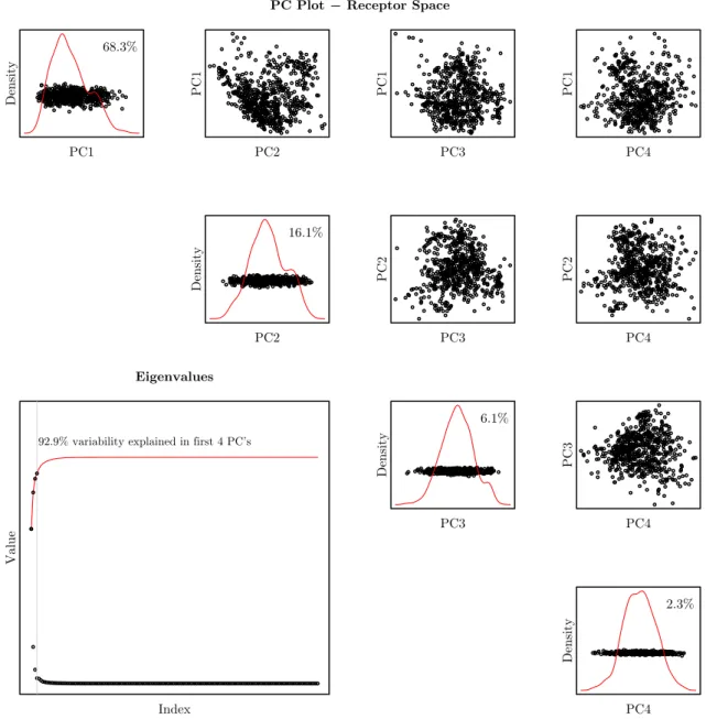
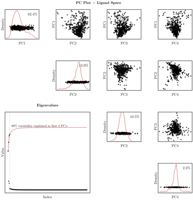
A useful characteristic of PCA is that it allows us to visualize and gain insight into how the data are distributed. This is especially useful when the data is in a higher dimensional space. In Figures 1.6 and 1.7 we have plotted a scatterplot matrix showing the joint structure in the first four principal components as well as the eigenvalues for both proteins and ligands, respectively in the RLP800 training data set.

Figures 1.6 and 1.7 provide some insight into the distribution of the RLP800 data. Consider the plots of the eigenvalues in the lower left hand corner of each figure; what immediately stands out is the relatively small number of eigenvalues needed to explain a large proportion of the variation in both protein and ligand space. Here the proportion of variation measured by principal component i is given as

var(Xvi X) P

jvar(Xv

j X)

= γ

i X P

jγ j X

. (1.13)

(31)

2.3.

(32)

PC Plot − Receptor Space

Density

PC1 68.3%

PC1

PC2

PC1

PC3

PC1

PC4

16.1%

Density

PC2

PC3

PC2

PC4

6.1%

Density

PC3

PC4

2.3%

Density

PC4 Eigenvalues

92.9% variability explained in first 4 PC’s

Value

Index

(33)

PC Plot − Ligand Space

Density

PC1 62.4%

PC1

PC2

PC1

PC3

PC1

PC4

13.9%

Density

PC2

PC3

PC2

PC4

10.5%

Density

PC3

PC4

2.2%

Density

PC4 Eigenvalues

89% variability explained in first 4 PC’s

Value

Index

(34)

CHAPTER 2

A mapping between spaces: Canonical Correlation

Analysis

CCA was first proposed in 1936 (Hotelling (1936)). Since then it has seen application in a multitude of fields. In the prediction of protein-ligand binding the complexity of the data necessitates a way to model the relationship between them. CCA provides a natural framework for this type of analysis.

2.1 Linear Case

Consider the framework laid out in Section 1.1. Let ΣXX = cov(X, X), ΣY Y = cov(Y, Y) andΣXY = cov(X, Y) denote the population covariances andSXX =cov(c X,X),

SYY =cov(c Y,Y) and SXY =cov(c X,Y) the sample covariances.

Since correlation is scale invariant we can make an arbitrary normalization ofwX and

wY. With this in mind we have the constraint

cov(_hX,wX_i,_hX,wX_i) = cov(_hY,wY_i,_hY,wY_i) = 1 (2.1)

Using this constraint the optimization problem in (1.2) can be written as

ρ_H = max wX,wY

corr(_hX,wX_i,_hY,wY_i) =wTXΣXYwY,

(35)

Using Lagrange multipliers ρX and ρY the corresponding Lagrangian is

L(wX,wY, ρX, ρY) = wXTΣXYwY −

ρX

2 (w

T

XΣXXwX −1)−

ρY

2 (w

T

YΣY YwY −1). (2.3)

Taking the derivative of (2.3) with respect to wX and wY and setting equal to zero we have

∂L(wX,wY, ρX, ρY)

∂wX = ΣXYwY −ρXΣXXwX = 0, (2.4)

∂wY = ΣY XwX −ρYΣY YwY = 0. (2.5)

Multiplying the left hand sides of Equations (2.4) and (2.5) by, respectively, wT

X andwTY

and then subtracting the resulting equations from each other gives us

wXTΣXYwY −ρXwTXΣXXwX −wTYΣY XwX +ρYwTYΣY YwY

=ρYwTYΣY YwY −ρXwTXΣXXwX = 0,

from which it follows that

ρX =ρY = corr(hX,wXi,hY,wYi) = ρH.

Assuming ΣY Y is invertible we have

wY = Σ

−1

Y YΣY XwX

ρ_H . (2.6)

Similarly we have,

wX = Σ

−1

XXΣXYwY

ρ_H . (2.7)

Substituting (2.6) into (2.4) and rearranging terms gives the generalized eigenvalue prob-lem,

ΣXYΣ−Y Y1ΣY XwX =ρ 2

(36)

similar calculations lead to

ΣY XΣ−XX1 ΣY XwY =ρ2_HΣY YwY. (2.9)

Equivalently using Equations (2.4) and (2.5) the generalized eigenvalue problem can be rewritten as,

 

 0 ΣXY

ΣY X 0   

 

 wX

wY  

=ρ_H

 

 ΣXX 0

0 ΣY Y

  

 

 wX

wY  

. (2.10)

We now discuss how to find second and subsequent linear combinations ofX andY. The objective is to find maximally correlated linear combinations ofX, sayXw∗

X and Y, say

Yw∗

Y which are uncorrelated with XwX andYwY from (2.2). The optimization problem

thus written as,

ρ_H = max w∗

X,w

∗

Y

corr(_hX,w∗_X_i,_hY,w_Y∗_i) = (w∗_X)T_Σ

XYwY∗,

subject to

(w∗X)TΣXXwX∗ = (w∗Y)TΣY Yw∗Y = 1 wT

XΣXXw∗X =w

T

YΣY YwY∗ = 0 wTXΣXYw∗Y =w

T

YΣY XwX∗ = 0.

(2.11)

Using Lagrange multipliers ρ∗

X, ρ∗Y, µX and µY gives the Lagrangian,

L(wX∗,w∗Y, ρ∗X, ρ∗Y, µX, µY) = (wX∗ ) T

ΣXYw∗Y −

ρ∗

X

2 ((w

∗

X) T

ΣXXwX∗ −1)

−ρ₂∗Y ((wY∗)TΣY YwY∗ −1) +µXwTXΣXXw∗X +µYwYTΣY Yw∗Y. (2.12)

Taking the derivative of (2.12) with respect w∗

(37)

have,

∂L(w∗

X,w∗Y, ρ∗X, ρ∗Y, µX, µY)

∂w∗

X

= ΣXYwY∗ −ρ∗XΣXXwX∗ +µXΣXXwX =0, (2.13)

∂L(w∗

X,w∗Y, ρ∗X, ρ∗Y, µX, µY)

∂w∗

Y

= ΣY Xw∗X −ρ∗YΣY Yw∗Y +µYΣY YwY =0. (2.14)

Multiplying the left hand side of (2.13) and (2.14) by wT

X and wTY respectively gives us

0 =µXwXTΣXXwX =µX,

0 =µYwTYΣY YwY =µY.

With µX = µY = 0 it can be seen that the canonical vectors wX∗ and wY∗ are the

second set of eigenvectors from the generalized eigenvalue problem in (2.8) and (2.9). The extension to additional linear combinations ofX and Y follows along the same lines as just described with the constraints in (2.11) being modified to include orthogonality to all previous linear combinations ofX and Y.

Remark 2.1.1. Eigen analyses have ambiguous polarity in the sense that they are only determined up to a factor of_±1. This ambiguous polarity is resolved in a way that gives comparable results across similar data analyses by employing the following convention: The main idea is that the directions the eigenvectors follow, in each space, will always place the largest, in absolute value, projected value across both spaces on the positive (right hand) side of the axis. In other words let X, Y, wX and wY be as defined previously. Define the scores ai

X =xTiwX and aiY =yTi wY to be the projected values of

the ith _{observation onto its canonical vector. Let} _a(n)

X and a

(n)

Y be the largest score, in

absolute value, across all ak

X and a

k

Y, k = 1, . . . , n, respectively. Then,

aiX = sign(max{a (n) X , a

(n) Y })·a

i X,

ai

Y = sign(max{a (n) X , a

(n) Y })·a

i Y.

(38)

In the event of a tie in the scores a(Xn) and a (n)

Y the sign is taken to be +1. This

transfor-mation of the data does not change the relationship of the projections between spaces. This can be seen by noting that the values of the signs by which we are multiplying the projections in both spaces will always be the same. Thus the correlation between the projections will remain unchanged.

An example of linear CCA was presented in Section 1.2. In the following section we present several toy examples illustrating where linear CCA performs well and also where it does not perform well.

2.2 Properties of CCA

CCA is invariant with respect to several common linear transformations. This point is illustrated in Figure 2.1. Plots (b), (c) and (d) in Figure 2.1 depict different transfor-mations, orthonormal, scale and location, respectively of the data shown in Figure 2.1 (a) (not shown in the plots are the canonical correlations, 1 and 0.996 which are the same for all four groups of plots). These properties are straightforward to verify. Let X, Y,

wX and wY be defined as above. To ease calculation we also assume thatX and Y have mean zero.

1. Orthonormal: DefineQX _∈RdX×dX andQY ∈_RdY×dY to be orthonormal matrices.

I.e.:

(a) QT

XQX =QXQTX =IdX,

(b) QT

YQY =QYQTY =IdY

Define the orthonormal transformations X∗ ₌ _X_QX _and _Y∗ ₌ _Y_QY_{. Define E[}_·_]

to be the expected value. Using the result found in (2.8) we have

E[(X∗)T_Y∗_](E[(Y∗₎T_Y∗_])−1_E[(Y∗₎T_X∗_]_w∗

(39)

Substituting in for X∗ _and _Y∗ _{gives us,}

QT

XE[XTY]QY(QTYE[YTY]QY)−1QTYE[YTX]QXw∗X = (ρ∗)2QTXE[XTX]QXwX∗.

(2.17) Next we use properties (a) and (b) defined above. Multiplying the left hand side of the previous equation by QX and setting w′

X =QXw∗X gives us,

ΣXYΣ−Y Y1ΣY XwX′ = (ρ∗)2ΣXXw′X. (2.18)

From this it can be seen that the resulting generalized eigenvalue and eigenvector from (2.18) will be the same as those found in (2.8).

Figure 2.1(b) illustrates CCA’s invariance to orthonormal transformations. In the X space the data has been rotated 30◦ _{counterclockwise and in the Y space the data}

has been rotated 75◦ _{clockwise (these rotations satisfy the properties (a) and (b)).}

The resulting projected values remain unchanged as do the canonical correlation values.

2. Scale: We use the results from CCA’s invariance to orthonormal transformations to show its scale invariance. This follows immediately by substituting in scalars a and b for the orthonormal matrices QX and QY in (2.17) which then leads to the same result as in (2.18).

An illustration of CCA’s scale invariance is presented in Figure 2.1 (c). The pro-jected values and canonical correlations are identical to those in Figure 2.1 (a). 3. Translation: Define cx _∈Rd_X _and _cy _∈Rd_Y _{to be vectors of constants, and} _1n _∈Rn

to be a vector of ones then

corr(_hX+1cT

x,wXi,hY +1c T

(40)

=wXTE[X T

Y]wY

= corr(_hX,wX_i,_hY,wY_i).

Figure 2.1(d) provides an illustration of CCA’s invariance to translation. Looking at the projected values and canonical correlations they are identical to those found in (a).

2.3 Regularized Canonical Correlation Analysis

There are many cases, particularly in biological problems where the data being an-alyzed have a large number of covariates (descriptors) as compared to the number of observations. This can lead to situations where there are potentially many highly corre-lated covariates, this type of behavior is referred to as multicollinearity. An approach to control the effects of multicollinearity is to add a penalty term which controls the vari-ability of the eigenvectors of the sample covariance matrices within the X and Y spaces. There is a close relationship between variability in the eigenvectors and multicollinearity (which we discuss in greater detail below).

Recall that the eigenvalues and eigenvectors found from the eigen decomposition of the sample covariance matrixSXX (andSY Y) are also the solution to the PCA optimization problem discussed in Section 1.3.2.

(41)

vectors wX and wY can be written as,

wX = S

−1

XXSXYwY

ρ_H ,

wY = S

−1

Y YSY XwX

ρ_H .

The effect of this instability on the canonical vectors can be seen by noting that their solutions depend on the inverse of the covariance matricesSXX and SY Y. An immediate consequence of this is that when the sample eigenvalues act as just mentioned it can be seen from (2.19) that small eigenvalues (near zero) will tend to inflate the elements of these matrices,

S−_XX1 =VXD−_X1VT X, S−_{Y Y}1 =VYD−_Y1VT

Y.

(2.19)

Here VX = (v1

X, . . . ,v dX

X ) and VY = (vY1, . . . ,v dY

Y ) are the matrices of eigenvectors

(i.e. principal component direction vectors) of the sample covariance matrices SXX and

SY Y. The matrices D−X1 and D−Y1 have elements γ1i

X, i= 1, . . . , dX and 1 γi

Y, i= 1, . . . , dY

along their diagonals, where γi

X and γYi are the eigenvalues of their respective covariance

matrices.

(42)

co-sample and a significant deviation from the theoretical direction.

The impact of this variation is felt the strongest when projecting new data onto one of these directions. For example, suppose new observations are generated from a distribution similar to that just described with the difference lying in a slight perturbation of the covariance matrix in the X space. These new observations are then projected onto the canonical vectors shown in Figure 2.2.

Ideally the projected values of the new data would vary only slightly from one set of directions to the next. Figure 2.3 shows a plot of each pair of projected values (the projection of the new data discussed above onto each of the directions shown in Figure 2.2) against one another. The observations within each of these plots should, if the directions were well behaved, fall on or near the 45◦ _{line (shown in red). However, due}

to the large amount of variation in the canonical vectors the resulting projections are highly variable.

One possible approach to dealing with this problem is to control how variable we allow the canonical direction vectors to be. One such penalty would be a modification of the constraint in (2.1) where an L2 constraint on theL2 length of the canonical vectors wX and wY (Vinod (1976)) is added. This new constraint (2.20) now penalizes for how variable we allow the directions in any one space to be,

cov(_hX,wX_i,_hX,wX_i) +κXhwX,wXi= cov(hY,wYi,hY,wYi) +κYhwY,wYi= 1.

(2.20) Solving (2.2) but with new constraints (2.20) is done in a similar fashion to standard CCA. Using Lagrange multipliersρX and ρY we have the following modified Lagrangian

as compared to (2.3),

L(wX,wY, ρX, ρY) = wTXΣXYwY −

ρX

2 (w

T

XΣXXwX +κXwXTwX −1)

− ρY

2 (w

T

YΣY YwY +κYwTYwY −1).

(43)

Taking the derivative with respect to wX and wY and setting equal to zero gives

∂wX = ΣXYwY −ρX(ΣXXwX +κXwX) = 0, (2.22)

∂wY = ΣY XwX −ρY(ΣY YwY +κYwY) = 0. (2.23)

Multiplying the left hand sides of Equations (2.22) and (2.23) by, respectively, wT

X and

wT

Y and then subtracting the resulting equations from each other gives us

wT

XΣXYwY −ρX(wTXΣXXwX +w T

XwX)−w

T

YΣY XwX +ρY(wYTΣY YwY +wYTwY)

=ρY(wYTΣY YwY +wTYwY)−ρX(wTXΣXXwX +wTXwX) = 0,

from which it follows that

ρX =ρY = corr(hX,wXi,hY,wYi) = ρ_H.

Assuming ΣY Y +κYIdY is invertible we have

wY = (ΣY Y +κYIdY)−

1_Σ

Y XwX

ρ_H .

Substituting into (2.22) and rearranging terms gives the generalized eigenvalue problem,

ΣXY(ΣY Y +κYIdY)

−1_Σ

Y XwX =ρ2_H(ΣXX+κXIdX)wX, (2.24)

similar calculations lead to

ΣY X(ΣXX+κXIdX)

−1_Σ_{Y XwY} ₌_ρ2

H(ΣY Y +κYIdY)wY. (2.25)

(44)

rewritten as,

 

 0 ΣXY

ΣY X 0   

 

 wX

wY  

=ρ_H

 

 ΣXX +κXIdX 0

0 ΣY Y +κYIdY

  

 

 wX

wY  

. (2.26)

Subsequent calculations to find new directions are similar to those discussed for the un-penalized case. In addition the same invariance properties that were discussed for standard CCA hold for this regularized variant of CCA (RCCA).

Consider again the example presented at the beginning of this section. Figure 2.4 shows a plot of the canonical direction vectors found from using RCCA with a value of 0.1 for the regularization parameterκX. In contrast to Figure 2.2, the canonical direction

vectors are quite similar from one sample to the next. The dashed red line is once again the theoretical direction.

Figure 2.5 is the same plot as Figure 2.3 but with the new data being projected onto the direction vectors shown in Figure 2.4. As can be seen the projected values are quite similar from one set of directions to the next.

In the context of the protein-ligand matching problem consistent behavior of the canonical vectors is critical. Because the primary object of interest is the prediction of new protein-ligand pairs it is important that the directions that are found are not overly dependent on the training sample. As is illustrated in Figure 2.3 if measures are not taken to control the variability of the canonical vectors the projected values and any prediction based on them become unreliable.

2.4 A Toy Example

(45)

complex relationship between proteins and ligands. Recall the task is the following: given a new observation in the space of proteins can we accurately predict the corresponding point in the space of ligands.

The data in the space of proteins falls into three distinct groups and the data in the space of ligands falls into two distinct groups. This scenario is relevant in the context of our example for the following reason: a single protein can bind many different ligands, based on the conformation, i.e. steric layout, of the binding site. Thus in the context of our example the three different clusters could be thought of as representing three different proteins. The slight perturbation in each group is attributed to the change in conformation of the binding sites of each protein to allow the binding of different ligands. The two groups in the space of ligands could be thought of as representing ligands corresponding to proteins, larger macro molecules or shorter sequences of peptides, small molecules.

The data has been generated such that those points which fall into the same group in both protein and ligand space are highly correlated. The result is that the global structure of the data is non-linear in the following sense: the underlying correlation structure of protein ligand pairs is localized, as a result this relationship cannot be captured by a simple (global) linear combination of the descriptors.

Observations in Figure 2.7 are highlighted according to whether they fall into the same cluster in both spaces. This plot helps illustrate just how different the neighborhood structures are in protein space versus ligand space. Consider, for example, the point labeled 1a7t (cyan). Its neighbors in protein space are all different from the corresponding point in ligand space.

(46)

canonical directions, shown in red in the top row of plots in Figure 2.8, do not show a strong alignment of points between spaces. The same is true for the second canonical direction, shown in green in the bottom set of plots. The canonical correlation values, 0.46 and 0.34 confirm our visual assessment.

Looking at the projections onto the first two canonical vectors shown in Figure 2.9 we can see little if any change has been made to the structure of the data in protein space, relative to the raw data shown in Figure 2.6. In ligand space the directions found appear to have made the prediction of Lnew worse.

In Chapter 3 a variant of CCA will be discussed which can capture this non-linear relationship between spaces.

2.5 Connection Between Linear Discriminant

Anal-ysis and CCA

A question of interest in many problems is the classification of a set of observations into one of several distinct categories. This is one example of supervised learning, see Duda et al. (2000) for an overview of the large literature on this topic. In contrast to supervised learning is clustering, a specific area of unsupervised learning. In clustering the categories are unknown and the task is to determine what “natural” groupings can be found in the data. Linear Discriminant Analysis (LDA) (Fisher (1936)) is a standard tool used in classification. In Section 2.5.1 we outline LDA and in Section 2.5.2 we show LDA in terms of CCA.

2.5.1 Linear Discriminant Analysis

Consider the k class (i.e. k category) discrimination problem. Suppose we have a set of n observation-label pairs, (xi,yi) _∈ Rd_{× {}_0,₁_}k_, _i _{= 1, . . . , n. Let} _C_j_, _j _{= 1, . . . , k}

(47)

let the observations xi be a collection of drug descriptors (i.e. ligands) and yi be the labels representing whether a drug is active or inactive. DefineX _∈Rn×d _{to be a matrix}

whose rows are the observations xi. Define Y _∈Rn×k _{to be the label matrix whose}_ijth

entry is defined as yij =I{xj∈Ci}, whereI is the indicator function. One way to think of

LDA is that it looks to find a vector of weights, wX, associated with the columns of X, such that the linear combination,XwX maximizes the ratio of its between-class variance to its within-class variance, defined in (2.30) and (2.29). To ease notation we assume that X has been mean centered.

Definenj =P_iyij =|Cj|, where|Cj| denotes the cardinality ofCj, to be the number

of observations in classj and let mj in (2.27) be defined as the mean of the observations that belong to class j,

mj = 1

nj X

i:xi∈Cj

xi. (2.27)

Define the total sum of squares to be

ST =

k X

i=1 X

j:xj∈Ci

xjxTj = (n−1)SXX, (2.28)

where SXX is the sample covariance matrix, discussed in Section 2.1. The total sum of squares, ST can be decomposed into the sum of thewithin-class sum of squares,

SW =

k X

i=1 X

j:xj∈Ci

(xj₋mi)(xj ₋mi)T, (2.29)

and between-class sum of squares

SB =

k X

i=1

nimimTi. (2.30)

Specifically,

(48)

With these definitions we can now state the LDA optimization problem,

w∗_X = arg max wX

wT

XSBwX,

subject to,

wT

XSWwX = 1.

(2.32)

Using the Lagrange multiplierλ gives the corresponding Lagrangian

L(wX, λ) = wT

XSBwX −λ(wTXSWwX −1). (2.33)

Taking the derivative of (2.33) with respect to wX and setting equal to zero gives us,

∂L(wX, λ)

∂wX =SBwX −λSWwX =0,

which yields the following generalized eigenvalue problem,

SBwX =λSWwX. (2.34)

Points are then projected onto the resulting eigenvectors wX giving x∗

i = xTi wX. An

observationx∗

i is assigned to a class based on which class centerm∗j =mTjwX,j = 1. . . , k

is nearest,

arg min_j_||x∗

i −m∗j||2 (2.35)

We show that for the two class problem a simple closed form solution exists for the direction wX.

Theorem 2.5.1. Given the optimization problem in (2.32) when the number of classes

k is equal to 2 then

w∗X =

1

√

λ∗S −1

(49)

where λ∗ ₌ nλ n1n2.

Proof. First we observe that when the number of classes is equal to two the between-class sum of squares can be expressed as

SB = n1n2

n (m1−m2)(m1−m2)

T

.

For notational purposes we rewrite the generalized eigenvalue problem in (2.34) as

S∗BwX =λ∗SWwX, (2.37)

where S∗

B = (m1 −m2)(m1−m2)T. From the generalized eigenvalue problem in (2.37)

and using the constraints in the optimization problem (2.32) we have

λ∗ =wXTS∗BwX

=wT

X(m1−m2)(m1−m2)

T_wX

= √1

λ∗(m1−m2)

T

S−W1(m1−m2)(m1−m2)T

1

√

λ∗S −1

W(m1−m2).

Rearranging terms gives us

λ∗ = (m1−m2)TSW−1(m1−m2). (2.38)

Next, starting with the left hand side of (2.37) and substituting in for wX and S∗

B, we

have

S∗BwX =

1

√

λ∗(m1−m2)(m1−m2)

T

S−_W1(m1−m2)

(50)

Now looking at the right hand side of (2.37) we have

λ∗SWwX =λ∗_√1 λ∗SWS

−1

W(m1−m2)

=√λ∗₍_m₁₋_m₂_).

Thus we have shown that the left and right sides of (2.37) are equal. Also note that conditions in (2.32) are satisfied

wT

XSWwX =

1

λ∗(m1−m2)

T_S−1

WSWS−

1

W(m1−m2)

= (m1 −m2)

T_S−1

W(m1−m2)

(m1 −m2)TSW−1(m1−m2)

= 1.

From this we can see that (2.36) is an eigenvector of the generalized eigenvalue problem in (2.34). In order to show that this is in fact the leading eigenvector note that because the rank of the between-class scatter matrix is 1 there are at most 1 non-zero eigenvalues in the generalized eigenvalue problem (2.37). However, from (2.38) it is clear that λ∗

and therefore λ will be strictly positive so long as m1 6= m2 and SW is non-singular. Therefore we have that (2.36) is the leading eigenvector of (2.34).

2.5.2 LDA Solved by CCA

(51)

matrix of class labels), we have,

Y =

        

1n1 0 · · · 0

0 1n2 · · · 0

... ... ... ...

0 0 _{· · ·} 1nk

        

.

From this it is easy to see that,

SY X =YT_X ₌

        

n1mT1

n2mT2

... nkmT

k         

.

It follows that

S−Y Y1 = (Y T

Y)−1 =

         1

n1 0 · · · 0

0 1

n2 · · · 0

... ... ... ...

0 0 _{· · ·} 1

nk         

.

Using these results we have

SXYS−_{Y Y}1SY X =

k X

i=1

nimimT

i =SB (2.39)

Starting with

SXYS−1

Y YSY XwX =ρ2HSXXwX,

and using (2.28) and (2.39) this can be rewritten as,

The analysis and advanced extensions of canonical correlation analysis