1
OPTICAL GEOMETRY CALIBRATION METHOD FOR COMPUTED TOMOGRAPHY AND APPLICATIONS OF COMPACT MICROBEAM RADIATION THERAPY
Pavel Chtcheprov
A dissertation submitted to the faculty of the University of North Carolina at Chapel Hill and North Carolina State University in partial fulfillment of the requirements for the
degree of Doctor of Philosophy in the joint Department of Biomedical Engineering.
Chapel Hill 2016
Approved by: David Lalush Otto Zhou Jianping Lu Yueh Lee
iii ABSTRACT
Pavel Chtcheprov: Optical Geometry Calibration Method for Free Form Digital Tomosynthesis
(Under the direction of Jianping Lu and Otto Zhou)
Digital tomosynthesis is a type of limited angle tomography that allows for 3D information reconstructed from a set of X-ray projection images taken at various angles using an X-ray tube, a mechanical arm to rotate the tube, and a digital detector.
Tomosynthesis reconstruction requires the knowledge of the precise location of the detector with respect to each X-ray source.
Current clinical tomosynthesis methods use a physically coupled source and detector so the geometry is always known and is always the same. This makes it impractical for mobile or field operations. We demonstrated a free form tomosynthesis and free form computed tomography (CT) with a decoupled source and detector setup that uses a novel optical method for accurate and real-time geometry calibration.
We accomplish this by using a camera to track the motion of the source relative to the detector, which is necessary for 3D reconstruction. A checkerboard pattern is
iv
v
ACKNOWLEDGEMENTS
I would like to express my sincere gratitude to my advisors, Dr. Jianping Lu and Dr. Otto Zhou, for their support and motivation on all of my projects. Their insight and drive for innovation inspired and pushed me to new intellectual limits. I would like to thank Dr. Yueh Lee for introducing me to the Applied Nanotechnology Lab and for the vast clinical research applications that he brought forth, including the animal protocols for our experiments. I would like to thank Dr. David Lalush for his imaging expertise and his experience in CT reconstruction algorithms, without which this research would have no practical applications. And I would like to thank Dr. Hugon Karwowski, for not only being a great electronics teacher, but also a steadfast mentor who has pushed me to think of myself and my future in new ways.
I would also like to thank all of my lab mates who provided professional and emotional support over the past five years — Dental Team: Gongting Wu, Dr. Jing Shan, Dr. Enrique Platin, Allison Hartman, and Jabari Calliste. Apollo II Team: Dr. Sha Chang, Christy Inscoe, Lei Zhang, Dr. Mike Hadsell, and Phil Laganis. Gated MRT Team: Christy Inscoe, Lei Zhang, Dr. Laurel Burk, and Dr. Yueh Lee. FIGMRT Team: Christy Inscoe, Lei Zhang, Dr. Laurel Burk, and Dr. Hong Yuan, and Dr. Yueh Lee. I would also like to thank the Physics Instrument Shop for their continued expertise with construction and
vi
Also, I would like to thank my wife, Kelly, for her continued support during my time as a graduate student and her design efforts in making my work look visually appealing and not just scientifically correct – something I often overlook. I would like to thank her for proofreading my manuscripts and telling me when my descriptions assume the reader is as immersed in the project as I am. I would also like to thank my parents for pushing me to this moment, especially my dad who has been a constant source of inspiration from the time I was in my crib, watching him derive equations on his stacks and stack of notebooks.
vii
TABLE OF CONTENTS
ABSTRACT ... iii
ACKNOWLEDGEMENTS ... v
TABLE OF CONTENTS... vii
LIST OF FIGURES ... xi
LIST OF ABBREVIATIONS ... xvii
Chapter 1: Introduction ... 1
1.1 Tomosynthesis ... 1
1.2 Computed Tomography ... 4
Chapter 2: Geometry calibration method based on pattern recognition ... 7
2.1 Current Clinical Geometry Calibration Methods ... 7
2.2 Pattern Detection ... 8
2.3 Optical Geometry Calibration Method ... 9
2.4 Stationary Detector ...11
2.5 Moving Detector ...13
Chapter 3: Free Form Tomosynthesis ...24
3.1 Motivation ...24
3.2 Application ...25
viii
3.4 Blank Image Library ...33
3.5 Reconstruction ...34
3.6 Matlab Implementation ...35
CHAPTER 4: Intraoral Tomosynthesis...41
4.1 Motivation ...41
4.2 Application ...42
4.4 Future Development ...45
Chapter 5: Free Form Computed Tomography ...46
5.1 Motivation ...46
5.2 Imaging ...46
5.3 Matlab Implementation ...49
5.4 Experimental Validation ...53
Chapter 6: Conclusion and Discussion ...58
Appendix 1: Introduction To Microbeam Radiation Therapy ...61
1.1 Glioblastoma Multiforme ...61
1.2 Radiation Therapy ...63
1.3 Treatment Planning ...67
Appendix 2: Background on Field Emission ...70
2.1 Carbon Nanotube Field Emission ...70
2.2 Carbon Nanotube Field Emission X-ray Tubes ...72
ix
2.4 Compact Image Guided MRT System for Small Animal Treatment ...78
2.5 Desktop MRT System ...79
2.6 Fluorescence Imaging ...80
2.6.1 Abstract ...80
2.6.2 Motivation ...81
2.6.3 X-ray Fluorescence ...83
2.6.4 Methods ...84
2.6.5 Results ...87
2.6.5 Conclusions ...91
2.6.6 Discussion ...92
2.7 Physiologically Gated Microbeam Radiation ...97
2.7.1 Abstract ...97
2.7.2 Motivation ...98
2.7.3 Physiological Motion Monitoring ...99
2.7.4 Mechanical phantom ... 100
2.7.5 Mouse Model and Handling ... 101
2.7.6 Respiratory Gated Irradiation ... 101
2.7.7 Irradiation Protocols ... 103
2.7.8 Histology ... 104
2.7.9 Results ... 105
x
2.8 Microbeam Interaction Simulations ... 111
Appendix 3: Second Generation Desktop MRT (Apollo II) ... 115
3.1 Motivation ... 115
3.2 Specifications ... 115
3.3 Design ... 116
3.3.1 Tube ... 116
3.3.2 Anode ... 118
3.3.3 Cathode Assembly ... 119
3.3.4 Collimator ... 119
3.3.5 Enclosure ... 121
3.4 Current Status ... 124
xi
LIST OF FIGURES
Figure 1. Two FDA approved digital breast tomosynthesis systems:
GE SenoClaire and Hologic Selenia Dimensions. ... 1 Figure 2. Hologic Selenia Dimensions tomosynthesis system showing
the rotating gantry holding the source. ... 2 Figure 3. Image sets taken from our lab’s custom-made stationary
source array tomosynthesis systems. Left: Comparison of 2D mamo to a 3D tomo of breast tissue and the increase visiblity of a lesion inside the tissue. Right: A) photo of tooth phantom B) 2D radioagraph of phantom C-F) Slices of a tomo set showing various carries that are not
noticeable in B. Note the three roots in C and D that are hidden in B. ... 3 Figure 4. GE CT machine from
http://www3.gehealthcare.in/en/products/categories/computed-tomography. ... 4 Figure 5. Shepp–Logan phantom (left) and its sinogram (right).
Adapted from https://tomroelandts.com/articles/tomography-part-
3-reconstruction. ... 5 Figure 6. Bead phantom method of geometry calibration. ... 7 Figure 7. Camera calibration images using a checkerboard pattern in
different orientation. ... 8 Figure 8. Processed checkerboard pattern image with the black square
intersections highlighted along with the coordinate system axes. ... 9 Figure 9. Setup modeled in Solidworks showing the camera and source
attachment with the pattern and detector assembly...10 Figure 10. Camera/source motion about an object and camera views of
the pattern at each position ...10 Figure 11. Source, Camera, Detector, and Pattern setup. ...11 Figure 12. Two views of source to camera vector lines plotted in CC
with the average vector in red. ...13 Figure 13. Sample large angle tomo setup diagram. ...14 Figure 14. Camera centric and pattern centric views of three images
xii
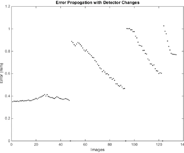
Figure 17. Error propagation simulation showing the absolute position
error (in mm) accumulating with each position change. ...23 Figure 18. Portable, handheld X-ray security imaging devices by NOVO
Digital Radiography http://www.novo-dr.com/. ...25 Figure 19. Flow chart of free form imaging process. ...26 Figure 20. Setup using the Carestream DRX Revolution mobile imaging
unit. Left: Camera mounting bracket and safety tape holding lose USB Right: Detector with optical pattern placement and beads (attached post
imaging to relate pattern to detector). ...28 Figure 21. Percent of the field of view taken by the pattern board vs accuracy. ...29 Figure 22. Two camera accuracy in the X-Y plane. ...30 Figure 23. Speed graph during horizontal motion tracking on a 2.5mm/s
translation stage showing the average calculated speed. ...30 Figure 24. 3D representation of the camera and source positions (numbered
dots) relative to the detector. The source and camera were positioned by
hand about the detector and are not meant to follow a perfect arc. ...31 Figure 25. Slices 7, 20, and 63 using the geometry phantom source
position data (top) compared to the optically calculated source positions
(bottom) showing the wire and different beads in focus. ...32 Figure 26. Horizontal and vertical profiles of the optically reconstructed
bar in the phantom images 635 μm ...32 Figure 27. Five slices through a foot from free tomo acquisition (source
was manually moved to 11 positions across an ~15º arc) ...34 Figure 28. Sets of 3 images from 2 depths of reconstruction tomo sets
of a hand. First image in each set was taken by the stationary chest tomo, second was on the free tomo setup using the geometry phantom to calculate the source position and the third was using the optical
calibration geometry ...34 Figure 29. Webcam acquisition GUI ...38 Figure 30. Screenshot of the Camera Calibrator App in Matlab loaded
with an image set. ...39 Figure 31. Output of the showExtrinsicsDATA_SET_NAME_CALIB.m file.
The “error” from the predicted value to the “actual” value of the geocal phantom, the calibration pixel error, the vectors averages to show the CS vector, and the camera and source positions plotted relative to the
xiii
Figure 32. Oral tomosynthesis setup using a custom made holder with the checkerboard pattern and with the optical camera attached
on the X-ray housing. ...43 Figure 33. Illustration of bead phantom calibration problem with a
small detector relative to the source to detector distance. The detector pixel size of 33µm creates an uncertainty shown on the left that results
in a much larger 1.6mm source uncertainty shown on the right. ...44 Figure 34. Camera attached to dental X-ray unit and imaging a dental
phantom with the custom made detector and pattern holder. ...44 Figure 35. Flowchart showing the imaging cycle of the free form tomo
imaging. ...47 Figure 36. A) Free form CT imaging setup with the object rigidly
attached to not move during the process to a low attenuating rod (meter stick). B) Imaging begins at the left side. C) Reaching the limit of this detector position. D) Source is stationary, the detector is moved to preserve the coordinate system. E) Imaging continues to the right-most side with the detector flat. F) Source is stationary, the detector is moved once again and the imaging can continue to the
right side. ...48 Figure 37. Reconstructed patterns and camera coordinate systems of a
desktop proof of concept to show the program working. The rainbow
colored rectangle is the starting pattern position. ...53 Figure 38. Reconstructed camera and source positions on a CT data set.
The dark blue lines are the z-axes of the camera (pointing directly out
perpendicular to the lens) and the asterisks are the calculated source positions. ...54 Figure 39. Side and top projection views of the security phantom. ...55 Figure 40. Top: Projection image of the circuit board showing no depth
information regarding the serial pins on the left. Bottom: Photo of the
serial pins. ...56 Figure 41. Slices 3 and 17 (at 0.2mm slice thickness) focusing on the
top and bottom pins of the serial connection. The slice separation is 2.8mm (at the 0.2mm resolution) indicating the same separation between the top and bottom rows. The datasheet on the right shows
the actual distance to be 2.84mm. ...56 Figure 42. Line profile of the chip pins showing the expected increase
in contrast in the tomo slice due to the removal of attenuating layers
xiv
Figure 43. X-ray Scanning Robot from the First Responders Group in DC.
http://www.firstresponder.gov/TechnologyImages/X-Ray%20Scanning%20Rover/x%20ray%20rover.jpg ...60 Figure 44. Schematic of a CNT field emission X-ray source. ...74 Figure 45 Spacial distribution of X-rays around a thin target.
F. Khan, "Total body irradiation," The physics of radiation therapy.3rd
ed.Philadelphia: Lippincott Williams & Wilkins, 455-463 (2003).. ...75 Figure 46. MRT beam visualization using a crosshatched irradiation pattern ...76 Figure 47. a) Isolated view of the cathode assembly showing the 5
cathodes producing a focal line on the anode. b) Side cutaway view of the MRT tube showing the electron beam from the cathodes hitting
the anode and producing the fan beam which is then collimated ...80 Figure 48. X-ray fluorescence illustration ...83 Figure 49. X-ray fluorescence setup with the Amptek spectrµm analyzer,
the slit collimator, MRT beam positioned directly through the collimator
slit, and the sample. ...85 Figure 50. Illustration of the MRT XRF imaging system. The subject is
slowly scanned through the MRT beam and the fluorescent signal from the iodine in that slice is recorded and processed. The output is an iodine
concentration vs position graph corresponding to the tumor location. ...87 Figure 51. Iodine fluorescence spectrµm showing the k alpha peak at
28.6 keV ...88 Figure 52. Fluorescent signal vs position of 0.2 mm/step, 20 s/step
cylindrical phantom ...89 Figure 53. Mouse in holder with Gafchromic X-ray sensitive film
showing the starting radiation beam location ...89 Figure 54. Fluorescent signal vs position graph overlaid on a sagittal
projection X-ray. 1 minute perfusion; 1 mm/step, 20 s/step, 80mm
total scan distance ...90 Figure 55. Fluorescent signal vs position graph overlaid on a CT
sagittal projection with color marked organs. 10 minute perfusion;
1mm/step, 20 s/step, 90 mm total scan distance ...91 Figure 56. Schematic of phantom using servo motor arm simulating
mouse abdominal motion during breathing. The arm is always in contact with the foam pad and the pressure sensor and oscillates
xv
Figure 57. BioVet© differential pressure measurement, correlated
to chest displacement, compared to the phantom angular displacement. ... 101 Figure 58. X-ray exposure pulse diagram. The top is the BioVet©
output of the respiratory motion from the pressure sensor attached to the mouse. The green line is the threshold set by the operator at low as possible but still having the ‘motionless’ state below it. The second pulse sequence shows the delay pulses that start the
irradiation on a high-to-low trigger. The last sequence shows the cathode pulses that generate the X-rays. The cathodes are negatively
pulsed at 500 µs pulse widths with an 8% duty cycle. ... 103 Figure 59. Diagram of histology section plane ... 104 Figure 60. Single beam dose curves for three 5 minute irradiations at
160 kVp ... 106 Figure 61. Three beam dose curves for three 5 minute/line irradiations
at 160 kVp. ... 107 Figure 62. Mouse in the mouse bed post-treatment with MRT beam
lines shown on EBT2 Gafchromic© dosimetry film taped to bed. ... 108 Figure 63. γ-H2Ax staining of a liver cross section showing gated
and non-gated lines. The stained points show DNA double strand
breaks which is proportional to the dose delivered. ... 109 Figure 64. Plot profile of the γ-H2Ax stain in Figure 9. ... 109 Figure 65. Beam profiles at 3 radii: 1.25mm, 1.77m, and 3.54mm.
At the 1.25 radius: PVDR 4.2, 1.77mm radius: PVDR 7.3, 3.54mm
radius: PVDR 16.7 ... 112 Figure 66. Other simulated line geometries ... 113 Figure 67. PVDR vs Beam Spacing graph with a point at 900µm
showing a PVDR of 14.13 ... 114 Figure 68. Cross section of Apollo II showing the high voltage
feedthrough, anode, and brazed oil cooling feedthrough. Below the anode is the X-ray window and under it is the rotating, variable
beam width, three beam collimator. ... 117 Figure 69. Photo of the Apollo II Tube housing without any
electrical connections. ... 117 Figure 70. Anode operation showing the three electron beams
hitting the 3 rows on the anode and being collimated into three
xvi
Figure 71. Anode with attached oil tubes seen through the side
ports of the chamber. ... 118
Figure 72. Cathode assembly timing diagram comparison between Apollo I and II ... 119
Figure 73. Top and side view photos of the cathode assembly. ... 119
Figure 74. Adjustable multi-slit collimator design. ... 121
Figure 75. Solidworks model of the enclosure. ... 123
xvii
LIST OF ABBREVIATIONS
BIL – Blank Image Library
BNL – Brookhaven National Labs
CNT – Carbon Nanotube
GBM – Glioblastom multiforme
CT – Computed Tomography
ESRF – European Synchrotron Radiation Facility
FWHM – Full Width at Half Maximum
HVL – Half Value Layer
MRT – Microbeam Radiation Therapy
PVDR – Peak to Valley Dose Ratio
ROI – Region of Interest
RGA – Residual Gas Analyzer
RT – Radiation Therapy
SSD – Source to Surface Distance
SDBT – Stationary Digital Breast Tomosynthesis
SDCT – Stationary Digital Chest Tomosynthesis
1
CHAPTER 1: INTRODUCTION 1.1 Tomosynthesis
Digital tomosynthesis is a type of limited angle tomography that allows for 3D information reconstructed from a set of X-ray projection images taken at various angles. Tomosynthesis allows a way to filter out the unwanted structure overlap and focus on a specific slice in the object1. The technology has been applied clinically for breast cancer screening and
diagnosis2, imaging of lung diseases3, and musculoskeletal imaging.
Figure 1. Two FDA approved digital breast tomosynthesis systems: GE SenoClaire and Hologic Selenia Dimensions.
Modern tomosynthesis tubes use a traditional X-ray tube, a mechanical arm to move the tube across an angular span, a digital detector, and a reconstruction algorithm that provides depth dependent X-ray images3. Digital tomosynthesis methods range from step
and shoot methods that move and stop at each angle to obtain a projection, continuous motion that takes images at each angle with the tube stopping, and the more recent
2
Figure 2. Hologic Selenia Dimensions tomosynthesis system showing the rotating gantry holding the source.
3
Figure 3. Image sets taken from our lab’s custom-made stationary source array tomosynthesis systems. Left: Comparison of 2D mamo to a 3D tomo of breast tissue and the increase visiblity of a lesion inside the tissue. Right: A) photo of tooth phantom B) 2D radioagraph of phantom C-F) Slices
of a tomo set showing various carries that are not noticeable in B. Note the three roots in C and D that are hidden in B.
X-ray tomosynthesis reconstruction requires the knowledge of the precise locations of the X-ray source and the X-ray detector with respect to the object being imaged for each projection view taken. In the current commercial tomosynthesis scanners this is
4 1.2 Computed Tomography
Computed tomography (CT) is another type of 3D X-ray imaging system. Unlike tomosynthesis that keeps one plane in focus and thus suffers the results of blurring from out of plane features, CT completely
eliminated artifacts from overlaying tissues7. The traditional way of taking a CT is to hold the source opposite a detector or series of detectors and to rotate the body, or the detector/source combination, about a stationary axis using a gantry. This produces a series of 2D projection images, which each horizontal 1D line
being a projection of a 2D axial cross-section of the object at the imaging projection angle. A typical clinical CT is shown in Figure 4.
Seven generations of CT were developed in an effort to improve performance and image quality. These range from different source collimations – fan beams and cone beams and the no longer produced pencil beams and different detector geometries – from single, multiple, to detector rings.
Two categories of reconstruction methods exist for CT – analytical and iterative. An example of an analytic reconstruction is the filtered backprojection (FBP) method that is also used in tomosynthesis reconstruction. FBP has an advantage for being
computationally efficient and numerical stable7
Figure 4. GE CT machine from http://www3.gehealthcare.in/en/products/categories/
5
There are a variety of FBP methods developed for each type of CT geometry, but the general idea is summing all of the projection images at each angle over the entire angular span. A projection image is the summation of attenuations along the X-ray beam, which is the line integral of the object at a particular slice, in the case of a fan beam. The entire set of these projections is the Radon transform of the object, again at the particular slice. . If we denote the object in space as a function 𝑓(𝑥, 𝑦), the integral denoting the projection
image is:
𝑔(𝑙, 𝜃) = ∫−∞∞ 𝑓(𝑥(𝑠), 𝑦(𝑠))𝑑𝑠 where 𝑥(𝑠) = 𝑙 𝑐𝑜𝑠𝜃 − 𝑠 𝑠𝑖𝑛𝜃 and 𝑦(𝑠) = 𝑙 𝑠𝑖𝑛𝜃 + 𝑠 𝑐𝑜𝑠𝜃. This is effectively taking a normal integral along a rotated plane – like the projection images7.
A visualization of the Radon transform is known as a sonogram, with the projections plotted as a function of the angle of acquisition. The projection images tell us the
attenuation over the X-ray beam path but not where along the path the attenuations were caused. To create an image, we can assign every point along the beam path the 𝑔(𝑙, 𝜃) value. This “smears” the projection image across the imaging space and produces what is known as a backprojection image:
𝑏(𝑥, 𝑦) = 𝑔(𝑥 𝑐𝑜𝑠𝜃 + 𝑦 𝑠𝑖𝑛𝜃, 𝜃)
Summing all of these smears over all of the rotation angles produces the backprojection summation image: 𝑓𝑏(𝑥, 𝑦) = ∫ 𝑏(𝑥, 𝑦) 𝑑𝜃
𝜋
0 . After this, a ramp filter acting as a high pass filter removes the blurring of the image caused by the summations of discrete images. This
Figure 5. Shepp–Logan phantom (left) and its sinogram (right). Adapted from
6
7
CHAPTER 2: GEOMETRY CALIBRATION METHOD BASED ON PATTERN RECOGNITION
2.1 Current Clinical Geometry Calibration Methods
A common geometry calibration method used for clinical imaging systems involves the use of a bead phantom - a three dimensional block with metal beads in precisely known positions in two or more planes normal to the vertical direction. The phantom is placed on the detector in essentially any position and an X-ray projection image is taken. By
comparing the two dimensional projection to the known three dimensional bead positions, the source position relative to the detector can be calculated using a linear projection method, as shown in Figure 6. The accuracy of this method is dependent on the accuracy of the bead positions, usually determined by a high resolution CT, the distance between the bead planes, and the ratio of the phantom height to the source-detector distance.
8 2.2 Pattern Detection
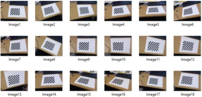
Pattern detection is a broad area of study in computer science. We focus specifically on optical pattern detection and further specify using the checkerboard pattern, which is popular with camera calibration techniques. There are a few calibration toolboxes out there, notably the OpenCV one by Jean-Yves Bouguet from Caltech
(docs.opencv.org/2.4/doc/tutorials/calib3d/camera_calibration/camera_calibration.html) and
the newer one from Matlab, included with their computer vision package. Camera calibration is necessary to measure and correct for the camera’s intrinsic, extrinsic, and lens-distortion parameters. This is accomplished by using a checkerboard pattern of known dimensions and taking a large set of images of it in different orientations. The algorithm creates the “perfect” pattern of known dimensions and using various rotation and skewing methods tries to fit the image to the modified ideal pattern. This can determine the skew, radial and tangential distortion of the lens, the principal point, and also the position of the
9
pattern relative to the focal point of the camera. This last bit of information is what we can use to do optical position tracking.
By providing an image set with a pattern, not only can one calibrate the camera to produce undistorted images, which though a useful feature in other research, does not provide us with any useful information, but one can use the calibration data to get the rotation and translation matrix data of the camera in the pattern coordinate system to < 0.2 pixels. Depending on the location of the pattern and your camera resolution, this can equate to sub-millimeter accuracy.
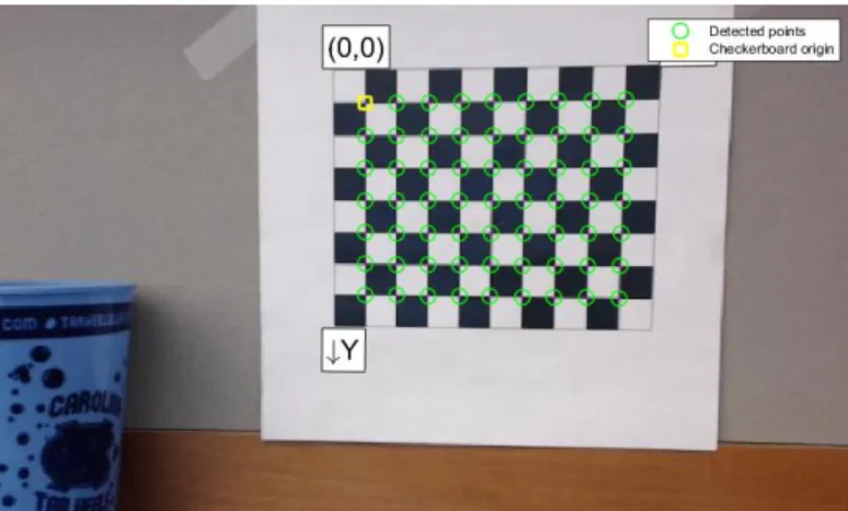
The image to the left in Figure 8 shows a processed checkerboard pattern image with an overlay of detected points and coordinate axes. It looks for the X intersection between the squares and creates a grid that it later matched to the ideal and known grid dimensions.
The coordinate system is also applied in the pattern space and shown here.
2.3 Optical Geometry Calibration Method
Here we present a method to perform three dimensional imaging using a decoupled source and detector without a rigid gantry or a predetermined source-detector trajectory. It uses an optical pattern recognition based method to accurately determine the imaging geometries of each projection images, in real time, for tomosynthesis reconstruction. The method can potentially allow tomosynthesis imaging to be performed in certain cases using a convention 2D imaging system with flexible and variable imaging geometry.
Figure 8. Processed checkerboard pattern image with the black square intersections highlighted along with
10
In a free form set-up, where the detector can be in any position relative to the source and moves from image to image, the relative positions of the source with respect to the detector need to be determined for each projection image. There are several ways to accomplish this using X-rays alone: placing the phantom on the detector alongside the object being imaged, putting the phantom, or markers, on the object and taking two images per position – one for calibration and one for the image set. The first cannot work if the object is as large as or larger than the detector and the second adds additional radiation.
Another option is to have a pattern of known size that is attached to the detector and tracked. The tracking allows for an accurate position of the pattern and the knowledge of the pattern’s position relative to the detector allows for the calculation of the position of
the detector. We accomplish this by using a camera to track the motion. The location is based on relative position change. The principle is as follows: a checkerboard pattern is positioned on or next to the detector using an extension arm in such a way that the
pattern will not move relative to the detector. A camera is mounted on the source in a way that the pattern is visible during imaging and will not move relative to the source, shown in Figure 9.
Figure 9. Setup modeled in Solidworks showing the camera and source attachment with the pattern and
detector assembly.
Figure 10. Camera/source motion about an object and camera views of the
11
The camera is then used to determine the source positions based on the orientation of the camera to the pattern. Figure 10 shows a sweeping source motion about an object and provides the camera view for each. The pattern rotation and position allows for an absolute position calculation to be performed. Checkerboard pattern recognition has been widely used in camera calibration and feature extraction and we use the same pattern for both in our procedure.
2.4 Stationary Detector
In the reconstruction, there are three coordinate systems: the camera (CC) that has the origin at the focal spot with the Z-axis being the vertical axis perpendicular to the lens pointing away from the camera, the detector (DC) that has the origin in the middle, with the positive X and Y axes being to the right and down respectively when looking at it from the top, and the pattern (PC) where the origin
is the top left corner intersection of the 4 squares with the X and Y axes in the same direction as with the detector. This assumes that the detector is stationary during the entire imaging process and creates the “world coordinate system” in which all of the above objects reside.
Using the computer vision library, the camera’s intrinsic parameters (lens
distortion, tangential skew, zoom) are obtained using a series of calibration images taken of the pattern in various positions/rotation. After this initial camera calibration is performed (unrelated to anything in the free form tomo system), the X-ray to camera calibration can
12
begin. The source/camera system is moved about the detector/pattern system, making certain neither component in each system is moved relative to each other, and an X-ray and corresponding optical image of the pattern is taken at each position. Using the intrinsic parameters from the initial calibration, the camera’s translation and rotation vectors can be obtained, which relate points in the camera coordinate system (𝑋𝐶𝐶) with points in the pattern coordinate system (𝑋𝑃𝐶) using the matrix transform:
𝑋𝐶𝐶= 𝑅𝑋𝑃𝐶+ 𝑡 (1)
From this, the camera position in the PC coordinate system can be obtained:
𝑋𝑃𝐶 = −𝑅−1𝑡 (2)
Next, DC needs to be related to PC. As the two are connected, their position can be determined in a number of ways. We assume that the two planes are parallel and their transform is a linear one, with 𝑀𝑋, 𝑀𝑌, 𝑀𝑍 being the linear offsets between DC and PC. This is true for our system where we control our pattern positioning. The transform can be applied to a randomly rotated/translated pattern to detector plane as well.
𝑋𝐷𝐶 = 𝑋𝑃𝐶− [
𝑀𝑥
𝑀𝑦
𝑀𝑧
] (3)
The final relation is the source position to the camera focal spot, after which the source position to the detector can be obtained from the above transforms. To do that, the calibration phantom is used to first get the source in the DC coordinate system. This is done using a standard geometry calibration phantom and ray tracing.
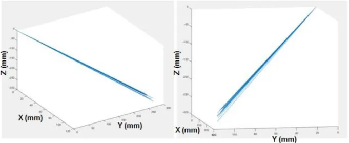
The calibration is completed by accurately getting the𝐶𝑆→ vector. From the geometry
13
all of the vectors from the origin (camera focal spot) to the source should theoretically all give the same vector, but due to measurement errors, gives slightly different results, shown plotted in Figure 12. Taking the average of those gives us the𝐶𝑆→ vector, shown in red.
Figure 12. Two views of source to camera vector lines plotted in CC with the average vector in red.
This completes the calibration procedure. From then, any new X-ray and
corresponding optical image can be processed to determine the position of the source to the detector. Using the𝐶𝑆→ vector and (1), the source in DC can be found by:
𝑆𝑜𝑢𝑟𝑐𝑒𝐷𝐶= 𝑅−1(𝐶𝑆 − 𝑡) − 𝑀 (4)
2.5 Moving Detector
14
Currently, the algorithm accounts for a stationary detector/object and looks at the camera projections relative to the detector. We can take an array of images at one detector position, move the detector about the body, and repeat the process and end up with multiple sets of projection images at multiple detector positions, but without a central coordinate system. A sample problem would be as follows: three projection images are taken for each detector position and the detector is rotated by 90º about the body, like the diagram in Figure 13.
Figure 13. Sample large angle tomo setup diagram.
15
each of the cameras relative to the detector (pattern in this sample case). This effectively gives the pattern and camera centric views, shown in Figure 14. The goal is to position the views of the detector positions 2 and 3 to reconstruct the original setup in Figure 13.
Figure 14. Camera centric and pattern centric views of three images taken at each detector position.
To accomplish this, there needs to be a link between the detector positions. Up until now, we have worked with the pattern centric setup and obtained positions of the cameras relative to the one detector. The key in linking the detector positions is switching the coordinate views and moving to a camera centric system during the detector move. This involves keeping the camera stationary and taking an image before the move and after the move, and then transferring the coordinate system origin back to the detector, only in its second position. This process is repeated for as many detector translations as necessary.
16
is moved to C2 while the detector is fixed and another image is taken. So far, the process is the same as before. Now we want to move the detector to D2. The camera is kept fixed at C2, the detector is moved to D2, and another image is taken (image 3) from C2. The
camera can then be moved (while the detector is again kept stationary in its new position at D2) to C4 and an image is taken. It is moved to C5 and another image is taken. We decide to move the detector again. The camera is held stationary at C4, the detector is moved to D3, and image 6 is taken. Now the camera is free to move about the detector as before.
Figure 15. Large angle tomosynthesis diagram.
17
There are 3 coordinate system families that are in play (Camera Coordinate - 𝑥̂𝑛′, Detector Coordinate - 𝑥̂𝑛, and the world coordinate system that the body lives in) in Figure 15.
Vector 𝑆⃗𝑎𝑏 represents the vector from a camera to its pattern origin, where a is the camera position (image #) and b is the coordinate system the image is associated with. Every 𝑆⃗𝑎𝑏 has and associated rotation matrix 𝑅𝑎𝑏 and translation vector 𝑡𝑎𝑏.
The coordinate transform from the camera coordinate system to detector is:
𝑋𝐶𝐶= 𝑅𝑋𝑃𝐶+ 𝑡 (5)
which is the position of the camera in image “a” in the 𝐷𝑏 coordinate system. 𝑆⃗21 and 𝑆⃗32 relate D1 and D2 because they are taken while the camera was stationary in the world coordinates. From this point, D1 is set at the origin of the world coordinates.
To find the locations of other points in D2, such as S4,2, and transform them into D1 (dubbed S4,1), we can follow the procedure: In 𝑥̂2′
𝑆⃗42𝑥̂
2 = 𝑅32(𝑆⃗42) + 𝑡32 (6)
where
𝑆⃗42= −𝑅42−1𝑡42 (7)
in 𝑥̂2described above. Transforming back into 𝑥̂1:
𝑆⃗42𝑥̂
1𝑎𝑙𝑠𝑜 𝑘𝑛𝑜𝑤𝑛 𝑎𝑠 𝑆⃗41= 𝑅21 −1(𝑆⃗
,2𝑥̂2) − 𝑡21= 𝑆⃗41= 𝑅21−1(𝑅32(𝑆⃗42) + 𝑡32) − 𝑡21 (8)
This is a recursive transform that must be taken at each new detector position. To do so, a list of all of the image numbers that precede a detector transition is necessary:
18
To find the position of the camera of image α which is in the coordinate system of Detector β, the following recursive function is used:
𝑆⃗𝛼,𝛽−1 = 𝑅𝛾,𝛽−1(𝑅𝛾+1,𝛽+1∗ 𝑆𝛼,𝛽+ 𝑡𝛾+1,𝛽+1− 𝑡𝛾,𝛽) (9)
Where γ is the maximum position number in steps that is less than α and β is its index position in ‘steps’ (which coincides with the D coordinate system). This is repeated until β=1 (in Detector 1 coordinate system, ie the world coordinates)
Now we take a look at the rotation matrices:
Figure 16. Rotation matrix between detectors illustration
Let 𝑢⃗⃗ =< 1,0,0 > the x axis in any coordinate system as illustrated above. 𝑢⃗⃗ in 𝑥̂2 can be written as
𝑊𝑢⃗⃗ + 𝑐1 in 𝑥̂1 (10)
Following our previous transform
𝑅21−1(𝑅32(𝑢⃗⃗) + 𝑡32) − 𝑡21= 𝑊𝑢⃗⃗ + 𝑐1 (11)
19
𝑊 = 𝑅21−1𝑅32 (13)
𝑐1= 𝑅21−1𝑡32− 𝑅21−1𝑡21 (14)
So to get the rotation matrix, for example, of R41, we would use: R41=R42*W2. We apply the same recursive technique as before for multiple detector transforms:
𝑊𝛽+1 = 𝑊𝛽∗ 𝑅𝛾+1,𝛽+1−1𝑅𝛼,𝛽 (15)
𝑊2= 𝑅32−1𝑅21 (16)
The next step is taking a look at the error propagation of this recursive function. Every camera position error relative to the detector is independent of the previous positions but every absolute position calculation from a camera position taken relative to a moved detector will have an increased error that propagated from the detector motion. From the recursive position formula 9, the maximum error will be on the last detector’s image set, so limiting the detector positions reduces the error.
From a single camera projection, the uncertainty is:
𝑠 = √(𝜕𝑆
𝜕𝑥) 2
𝑠𝑥2+ ( 𝜕𝑆 𝜕𝑦)
2
𝑠𝑦2+ ( 𝜕𝑆 𝜕𝑧)
2
𝑠𝑧2+ ( 𝜕𝑆 𝜕𝜃)
2
𝑠𝜃2+ (𝜕𝑆 𝜕𝜑)
2
𝑠𝜑2+ ( 𝜕𝑆 𝜕𝜓)
2
𝑠𝜓2 (17)
where θ, φ, and ψ are the Euler angles of the rotation matrix. The rotation matrix can be represented as a combination of the three coordinate axis rotations:
𝑅 = 𝑅𝑧(φ)𝑅𝑦(θ)𝑅𝑥(ψ) (18)
𝑅𝑥(ψ) = [
1 0 0
0 𝑐𝑜𝑠𝜓 −𝑠𝑖𝑛𝜓 0 𝑠𝑖𝑛𝜓 𝑐𝑜𝑠𝜓
20 𝑅𝑦(θ) = [
𝑐𝑜𝑠𝜃 0 𝑠𝑖𝑛𝜃
0 1 0
−𝑠𝑖𝑛𝜃 0 𝑐𝑜𝑠𝜃
] (20)
𝑅𝑧(φ) = [
𝑐𝑜𝑠𝜑 −𝑠𝑖𝑛𝜑 0 𝑠𝑖𝑛𝜑 𝑐𝑜𝑠𝜑 0
0 0 1
] (21)
𝑅 = [
𝑐𝑜𝑠𝜃 𝑐𝑜𝑠𝜑 𝑠𝑖𝑛𝜓 𝑠𝑖𝑛𝜃 𝑐𝑜𝑠𝜑 − 𝑠𝑖𝑛𝜑 𝑐𝑜𝑠𝜓 𝑐𝑜𝑠𝜓 𝑠𝑖𝑛𝜃 𝑐𝑜𝑠𝜑 + 𝑠𝑖𝑛𝜑 𝑠𝑖𝑛𝜓 𝑐𝑜𝑠𝜃 𝑠𝑖𝑛𝜑 𝑠𝑖𝑛𝜓 𝑠𝑖𝑛𝜃 𝑠𝑖𝑛𝜑 + 𝑐𝑜𝑠𝜑 𝑐𝑜𝑠𝜓 𝑐𝑜𝑠𝜓 𝑠𝑖𝑛𝜃 𝑠𝑖𝑛𝜑 − 𝑐𝑜𝑠𝜑 𝑠𝑖𝑛𝜓
−𝑠𝑖𝑛𝜃 𝑠𝑖𝑛𝜓 𝑐𝑜𝑠𝜃 𝑐𝑜𝑠𝜓 𝑐𝑜𝑠𝜃
] (22)
By expanding 17, the uncertainty becomes:
𝑠 = √ (𝑅 ( 1 0 0 )) 2
𝑠𝑥2+ (𝑅 (
0 1 0
))
2
𝑠𝑦2+ (𝑅 (
0 0 1
))
2
𝑠𝑧2+
(𝑑𝑅
𝑑𝜃𝑡) 2
𝑠𝜃2+ (𝑑𝑅
𝑑𝜑𝑡) 2
𝑠𝜑2+ ( 𝑑𝑅 𝑑𝜓𝑡)
2
𝑠𝜓2
(23)
𝜕𝑅 𝜕𝜃= [
−𝑠𝑖𝑛𝜃 𝑐𝑜𝑠𝜑 𝑠𝑖𝑛𝜓 𝑐𝑜𝑠𝜃 𝑐𝑜𝑠𝜑 𝑐𝑜𝑠𝜓 𝑐𝑜𝑠𝜃 𝑐𝑜𝑠𝜑 −𝑠𝑖𝑛𝜃 𝑠𝑖𝑛𝜑 𝑠𝑖𝑛𝜓 𝑐𝑜𝑠𝜃 𝑠𝑖𝑛𝜑 𝑐𝑜𝑠𝜓 𝑐𝑜𝑠𝜃 𝑠𝑖𝑛𝜑
−𝑐𝑜𝑠𝜃 −𝑠𝑖𝑛𝜓 𝑠𝑖𝑛𝜃 −𝑐𝑜𝑠𝜓 𝑠𝑖𝑛𝜃
] (24)
𝜕𝑅 𝜕𝜑= [
−𝑐𝑜𝑠𝜃 𝑠𝑖𝑛𝜑 −𝑠𝑖𝑛𝜓 𝑠𝑖𝑛𝜃 𝑠𝑖𝑛𝜑 − 𝑐𝑜𝑠𝜑 𝑐𝑜𝑠𝜓 −𝑐𝑜𝑠𝜓 𝑠𝑖𝑛𝜃 𝑠𝑖𝑛𝜑 + 𝑐𝑜𝑠𝜑 𝑠𝑖𝑛𝜓 𝑐𝑜𝑠𝜃 𝑐𝑜𝑠𝜑 𝑠𝑖𝑛𝜓 𝑠𝑖𝑛𝜃 𝑐𝑜𝑠𝜑 − 𝑠𝑖𝑛𝜑 𝑐𝑜𝑠𝜓 𝑐𝑜𝑠𝜓 𝑠𝑖𝑛𝜃 𝑐𝑜𝑠𝜑 + 𝑠𝑖𝑛𝜑 𝑠𝑖𝑛𝜓
0 0 0
21 𝜕𝑅
𝜕𝜓= [
0 𝑐𝑜𝑠𝜓 𝑠𝑖𝑛𝜃 𝑐𝑜𝑠𝜑 + 𝑠𝑖𝑛𝜑 𝑠𝑖𝑛𝜓 −𝑠𝑖𝑛𝜓 𝑠𝑖𝑛𝜃 𝑐𝑜𝑠𝜑 + 𝑠𝑖𝑛𝜑 𝑐𝑜𝑠𝜓 0 𝑐𝑜𝑠𝜓 𝑠𝑖𝑛𝜃 𝑠𝑖𝑛𝜑 − 𝑐𝑜𝑠𝜑 𝑠𝑖𝑛𝜓 −𝑠𝑖𝑛𝜓 𝑠𝑖𝑛𝜃 𝑠𝑖𝑛𝜑 − 𝑐𝑜𝑠𝜑 𝑐𝑜𝑠𝜓
0 𝑐𝑜𝑠𝜓 𝑐𝑜𝑠𝜃 −𝑠𝑖𝑛𝜓 𝑐𝑜𝑠𝜃
] (26)
𝑠 =
√ [
(𝑐𝑜𝑠𝜃 𝑐𝑜𝑠𝜑)2𝑠 𝑥2
(𝑐𝑜𝑠𝜃 𝑠𝑖𝑛𝜑)2𝑠 𝑥2
(𝑠𝑖𝑛𝜃)2𝑠 𝑥2
] + [
(𝑠𝑖𝑛𝜓 𝑠𝑖𝑛𝜃 𝑐𝑜𝑠𝜑 − 𝑠𝑖𝑛𝜑 𝑐𝑜𝑠𝜓)2𝑠 𝑦2
(𝑠𝑖𝑛𝜓 𝑠𝑖𝑛𝜃 𝑠𝑖𝑛𝜑 + 𝑐𝑜𝑠𝜑 𝑐𝑜𝑠𝜓)2𝑠 𝑦2
(𝑠𝑖𝑛𝜓 𝑐𝑜𝑠𝜃)2𝑠 𝑦2
] + [
(𝑐𝑜𝑠𝜓 𝑠𝑖𝑛𝜃 𝑐𝑜𝑠𝜑 + 𝑠𝑖𝑛𝜑 𝑠𝑖𝑛𝜓)2
(𝑐𝑜𝑠𝜓 𝑠𝑖𝑛𝜃 𝑠𝑖𝑛𝜑 − 𝑐𝑜𝑠𝜑 𝑠𝑖𝑛𝜓)2
(𝑐𝑜𝑠𝜓 𝑐𝑜𝑠𝜃)2
] +
([
−𝑠𝑖𝑛𝜃 𝑐𝑜𝑠𝜑 𝑠𝑖𝑛𝜓 𝑐𝑜𝑠𝜃 𝑐𝑜𝑠𝜑 𝑐𝑜𝑠𝜓 𝑐𝑜𝑠𝜃 𝑐𝑜𝑠𝜑 −𝑠𝑖𝑛𝜃 𝑠𝑖𝑛𝜑 𝑠𝑖𝑛𝜓 𝑐𝑜𝑠𝜃 𝑠𝑖𝑛𝜑 𝑐𝑜𝑠𝜓 𝑐𝑜𝑠𝜃 𝑠𝑖𝑛𝜑
−𝑐𝑜𝑠𝜃 −𝑠𝑖𝑛𝜓 𝑠𝑖𝑛𝜃 −𝑐𝑜𝑠𝜓 𝑠𝑖𝑛𝜃
] 𝑡)
2
𝑠𝜃2+
([
−𝑐𝑜𝑠𝜃 𝑠𝑖𝑛𝜑 −𝑠𝑖𝑛𝜓 𝑠𝑖𝑛𝜃 𝑠𝑖𝑛𝜑 − 𝑐𝑜𝑠𝜑 𝑐𝑜𝑠𝜓 −𝑐𝑜𝑠𝜓 𝑠𝑖𝑛𝜃 𝑠𝑖𝑛𝜑 + 𝑐𝑜𝑠𝜑 𝑠𝑖𝑛𝜓 𝑐𝑜𝑠𝜃 𝑐𝑜𝑠𝜑 𝑠𝑖𝑛𝜓 𝑠𝑖𝑛𝜃 𝑐𝑜𝑠𝜑 − 𝑠𝑖𝑛𝜑 𝑐𝑜𝑠𝜓 𝑐𝑜𝑠𝜓 𝑠𝑖𝑛𝜃 𝑐𝑜𝑠𝜑 + 𝑠𝑖𝑛𝜑 𝑠𝑖𝑛𝜓
0 0 0
] 𝑡)
2
𝑠𝜑2+
([
0 𝑐𝑜𝑠𝜓 𝑠𝑖𝑛𝜃 𝑐𝑜𝑠𝜑 + 𝑠𝑖𝑛𝜑 𝑠𝑖𝑛𝜓 −𝑠𝑖𝑛𝜓 𝑠𝑖𝑛𝜃 𝑐𝑜𝑠𝜑 + 𝑠𝑖𝑛𝜑 𝑐𝑜𝑠𝜓 0 𝑐𝑜𝑠𝜓 𝑠𝑖𝑛𝜃 𝑠𝑖𝑛𝜑 − 𝑐𝑜𝑠𝜑 𝑠𝑖𝑛𝜓 −𝑠𝑖𝑛𝜓 𝑠𝑖𝑛𝜃 𝑠𝑖𝑛𝜑 − 𝑐𝑜𝑠𝜑 𝑐𝑜𝑠𝜓
0 𝑐𝑜𝑠𝜓 𝑐𝑜𝑠𝜃 −𝑠𝑖𝑛𝜓 𝑐𝑜𝑠𝜃
] 𝑡)
2
𝑠𝜓2
(27)
If the camera is directly above the pattern and its axes align with the pattern’s coordinate axes:
𝑡 = [ 0 0 800
] 𝜃 = 0º 𝜑 = 0º 𝜓 = 0º (28)
𝑠𝑥 = 0.2mm 𝑠𝑦= 0.2mm 𝑠𝑧 = 0.6mm (29)
𝑠𝜃= 0.1º 𝑠𝜑= 0.1º 𝑠𝜓= 0.1º (30)
Gives an uncertainty vector:
𝑠 = [ 1.41 1.41 0.600
] (31)
Entering the following realistic parameters:
𝑡 = [ 50 50 800
] 𝜃 = 15º 𝜑 = 5º 𝜓 = 5º (32)
𝑠𝑥 = 0.2mm 𝑠𝑦= 0.2mm 𝑠𝑧 = 0.6mm (33)
22 Gives an uncertainty vector:
𝑠 = [ 1.40 1.38 0.670
] (35)
Trying a closer distance at 𝑡𝑧 = 500mm logically drops the uncertainty to:
𝑠 = [ 0.906 0.886 0.615
] (36)
The above is the uncertainty for a single position detector. Adding a second detector position complicates the position vector, obtained from (9) to:
𝑆⃗𝛼,1= 𝑅𝛾,1−1(𝑅𝛾+1,2∗ 𝑆𝛼,2+ 𝑡𝛾+1,2− 𝑡𝛾1) (37)
Following equation 17, the uncertainty now becomes:
𝑠 =
√
( 𝜕𝑆
𝜕𝑥𝑡𝛾,1) 2
𝑠𝑥2𝑡𝛾,1+ ( 𝜕𝑆 𝜕𝑦𝑡𝛾,1)
2
𝑠𝑦2𝑡𝛾,1+ ( 𝜕𝑆 𝜕𝑧𝑡𝛾,1)
2
𝑠𝑧2𝑡𝛾,1+
( 𝜕𝑆
𝜕𝑥𝑡𝛾+1,2) 2
𝑠𝑥2𝑡𝛾+1,2+ ( 𝜕𝑆 𝜕𝑦𝑡𝛾+1,2)
2
𝑠𝑦2𝑡𝛾+1,2+ ( 𝜕𝑆 𝜕𝑧𝑡𝛾+1,2)
2
𝑠𝑧2𝑡𝛾+1,2 +
( 𝑑𝑆
𝑑𝜃𝑅𝛾,1) 2
𝑠𝜃
𝑅𝛾,1
2 + ( 𝑑𝑆 𝑑𝜑𝑅𝛾,1)
2
𝑠𝜑2𝑅𝛾,1+ ( 𝑑𝑆 𝑑𝜓𝑅𝛾,1)
2
𝑠𝜓
𝑅𝛾,1
2 +
( 𝑑𝑆
𝑑𝜃𝑅𝛾+1,2) 2
𝑠𝜃
𝑅𝛾+1,2
2 + ( 𝑑𝑆 𝑑𝜑𝑅𝛾+1,2)
2
𝑠𝜑2𝑅𝛾+1,2 + ( 𝑑𝑆 𝑑𝜓𝑅𝛾+1,2)
2
𝑠𝜓
𝑅𝛾+1,2
2 +
(𝜕𝑆𝛼2 𝜕𝑥 )
2
𝑠𝑥2+ ( 𝜕𝑆𝛼2
𝜕𝑦 ) 2
𝑠𝑦2+ ( 𝜕𝑆𝛼2
𝜕𝑧 ) 2
𝑠𝑧2+ ( 𝜕𝑆𝛼2
𝜕𝜃 ) 2
𝑠𝜃2+ (𝜕𝑆𝛼2 𝜕𝜑 )
2
𝑠𝜑2+ ( 𝜕𝑆𝛼2
𝜕𝜓) 2
𝑠𝜓2
(38)
23
subtracting from the data obtained by introducing an error to the values: 0.0002 to the rotation matrix and 0.05 to the X and Y and 0.13 to the Z in the translation vector (the approximate errors from the calibration output data).
24
CHAPTER 3: FREE FORM TOMOSYNTHESIS 3.1 Motivation
We will now take a look at three implementations of the optical geometry calibration method, starting with a general free form tomosynthesis. As stated before, current clinical tomo systems all have either a fixed gantry for motion or are operating under conditions that prevent the source and the detector from moving relative to each other. While the process works reasonably well for systems stationed in dedicated spaces, it becomes cumbersome and often impractical for mobile and field operations. The heavy mechanical gantry needed for mechanical stability takes space and makes it difficult to design mobile tomosynthesis scanners that can be useful in situations where the patient cannot be easily transferred, such as those with neck trauma or severe burns. Finally, the fixed trajectory limits the imaging to a linear arc acquisition due to practical engineering constrains, which may not be the most efficient projection image set.
Using our method, we can perform tomosynthesis imaging using a decoupled source and detector without a rigid gantry or a predetermined source-detector trajectory. This can potentially allow tomosynthesis imaging to be performed in certain cases using a
25
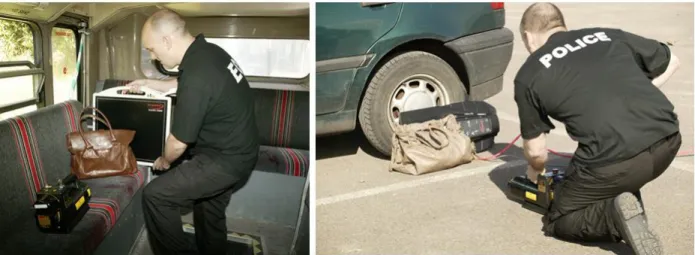
Figure 18. Portable, handheld X-ray security imaging devices by NOVO Digital Radiography http://www.novo-dr.com/.
There are methods that have been developed to accommodate imaging with a non-fixed detector. Gauntt et al. uses a motor control method of tube alignment8. The tube head has a six degree of freedom motor system that performs minor adjustments to the tube
position after approximate alignment by the technician. The alignment software looks at a
protruding cross shape with LEDs and its shape from the camera point of view determines
the necessary adjustments to be directly above the center of the detector8. Other methods
include using light patterns to position the detector in a predetermined orientation9,10
These all, however, attempt to position the detector to a specific orientation relative to the source. The calibration method will not only determine the source locations for reconstruction, but will also detect any motion during imaging and potentially still be able to reconstruct the images as every position for each image is known.
3.2 Application
26
parameters to be used during the optical reconstruction. The resolution was set to 1920 x 1080 with auto-focus turned off. Knowledge of the relative position of the camera relative to the source focal spot is necessary to perform the geometry calculation. For this one-time measurement, a standard metal bead calibration phantom that is suited to determine the absolute position of the source(s) to the detector for stationary tomosynthesis is used. The phantom is placed on the detector/pattern assembly and a few calibration X-ray and optical images are taken at different orientations. This provides the absolute source focal spot positions relative to the detector and the absolute optical focus spot position relative to the pattern. Since the position of the pattern relative to the detector is known, the position of the source can be determined relative to the optical focal spot. Once the camera/source system is calibrated, the phantom is no longer needed as the position of the pattern to the camera can be used to determine the position of the source to the detector. The method is summarized in the flowchart in Figure 19.
Figure 19. Flow chart of free form imaging process.
27
case the camera USB is ever pulled, which happens considering the source head’s range of motion, the pulling will hit the tape and not the actual camera, making sure the source and camera are always stationary relative to each other. This is a very important setup tip any time the camera is mounted on.
28
Figure 20. Setup using the Carestream DRX Revolution mobile imaging unit. Left: Camera mounting bracket and safety tape holding lose USB Right: Detector with optical pattern placement
and beads (attached post imaging to relate pattern to detector).
3.3 Accuracy
We tested the accuracy of the optical tracking by using a precision translation stage and moving the camera setup a known distance in three dimensions and then comparing those distance to the ones calculated by the system. This gave us a minimµm error threshold assuming perfection conditions. The conditions that affected the accuracy were also tested, including the distance from the pattern and the camera resolution.
29
X-ray geometry phantom and the optical geometry were used to reconstruct the calibration phantom. The comparison can be seen in Figure 25.
Feasibility testing was performed on a foot and hand phantom with the geometry calibration phantom next to each to compare reconstructions using the absolute geometry from the phantom and that obtained using the
optical imaging method. The geometry phantom was rigidly attached to the detector alongside the hand and foot.
The parameters contributing to accuracy that were investigated were the camera resolution and the distance from the pattern. The optimal resolution for the camera was found to be 1920x1080. Anything higher did not result in better accuracy and resulted in slower acquisition
time. The distance from the pattern played a major role but was also correlated with the pattern size so the better parameter to look at was the percentage of the image that was the pattern, which took into account both the distance and the pattern size. Unsurprisingly, it was found that the larger the pattern in the image, the smaller the error, as shown in Figure 21, so it was aimed to keep the pattern filling about 20% of the image during imaging. Two cameras were used to reduce the error, as seen in Figure 22. The error test in the X-Y plane showed the average error of less than 10μm using both cameras, with a maximum error of 400μm.
30
Figure 22. Two camera accuracy in the X-Y plane.
We also tested motion tracking accuracy using a continuous motion translation stages moving at 2.5mm/s. The camera frame rate was set to 1 fps and 20 images were taken and their geometry calculated. The plot of the average speed per step is recorded in Figure 23.
31
Figure 25 shows various slices of the geometry calibration phantom reconstructions using source position data obtains from X-ray projections (top) and from the optical
geometry calculations. Figure 26 shows the horizontal and vertical plot profiles of the wire from both reconstructions. The horizontal slice has a thickness of 604µm vs the actual 635µm – a 4.9% error for both reconstructions. The vertical profile thicknesses were 566µm and 547µm for the calibration phantom and optical respectively – 10.8% and 13.9% errors from the actual width and a 3.4% error between the two methods.
Figure 24. 3D representation of the camera and source positions (numbered dots) relative to the detector. The source and camera were positioned by hand about the detector and are not meant to
32
Figure 25. Slices 7, 20, and 63 using the geometry phantom source position data (top) compared to the optically calculated source positions (bottom) showing the wire and different beads in focus.
33 3.4 Blank Image Library
To appropriately reconstruct, the projection images need to be corrected according to the formula:
𝐶𝑜𝑟𝑟𝑒𝑐𝑡𝑒𝑑 𝐼𝑚𝑎𝑔𝑒 = 𝑅𝑎𝑤 − 𝐷𝑎𝑟𝑘 𝐵𝑙𝑎𝑛𝑘 − 𝐷𝑎𝑟𝑘
The dark image is an image taken with no X-ray to reduce the detector noise inherent to it. The blank image is taken at the same detector and source position as the raw but without the object. The raw image is the original image of the object obtained from the detector with no processing. This correction removes the non-uniform X-ray field caused by the source’s heel effect and detector orientation. In the standard case of a repeatable trajectory, this is a simple task. In the case of a manually positioned source and detector, one cannot take exact blanks before the object.
34 3.5 Reconstruction
The images were reconstructed using commercial filtered back projection software that allows for any source geometry to be input. Hand and foot phantoms were imaged through a manually positioned source, following the pattern seen above. Figure 7 shows the comparison between our stationary tomosynthesis device (left) and the reconstructions from the manual tomo (using a calibration phantom for source positioning in the middle and using our optically determined geometry on the right).
Figure 27. Five slices through a foot from free tomo acquisition (source was manually moved to 11 positions across an ~15º arc)
Figure 28. Sets of 3 images from 2 depths of reconstruction tomo sets of a hand. First image in each set was taken by the stationary chest tomo, second was on the free tomo setup using the geometry
35 3.6 Matlab Implementation
To perform the free tomo acquisition, processing, and reconstruction on RTT, several key programs and files are needed:
webcam.m: Found installed with the appropriate webcam drivers on the Applied Nanotechnology group laptop (C:\Users\User\Documents\MATLAB). If installing on another system, the line: handles.vid = videoinput('winvideo', 2, 'RGB24_1920x1080'); should be changed to the appropriate input channel, usually 1 if no other camera drivers are installed (such as a laptop webcam). This opens a GUI that allows the operator to take the images, check to make sure they are of good quality with a zoom ROI feature, retake if necessary, and save into the appropriate folder. Make sure to add the “\” at the end of the folder name. The images are saved numerically. Take an image and save it before every X-ray projection. A screenshot of the GUI is shown in Figure 29.
geometry.m: File that finds the source to detector geometry using the bead phantom. To speed up the acquisition, the calibration is performed using a subset of the actual data set. The bead geometry phantom is secured to the detector for all or part of the data collection for this reason and also to use as a comparison. Use the images with a good view of the bead phantom to get the geometry to use in the calibration
procedure. Returns geo.mat matrix that contains the course data. Check to make sure the values are not (0,0,0). If they are, that means not all of the points were found. Edit the thresholds on line: imfindcircles(image(1:range,1:2560),[10
36
a certain range but in 11, the object enters that range so from 11-something else, edit the new range to not include the object. Repeat as necessary.
cameraCalibration_DATA_SET_NAME.m: Partially auto-generated by
cameraCalibrator app. Can be used as a reference to create new ones for each image set. The initial calibration file can be generated from the Camera Calibrator App in Matlab. A screenshot of it is shown below in Figure 30. I recommend creating a new file for each set to keep track of them easier and if necessary modify to fit new conditions, such as: cameraCalibration_1_1_2015_XPhantom.m. This file is the calibration script for the camera to the source and should, later on, be only used once, but since the camera is added for every new experiment and removed, the calibration must be run for every new data set. Use at least 20 images to get a good calibration – both of the camera intrinsic parameters and the geometry. The file consists of: imageFileNames – an array of the optical images ONLY used for the recon – not the entire set. offX=183.48-355.84/2; offY=24.05-427.01/2; are the pattern offsets relative to the detector found using the beads as described and illustrated in Figure 20. [poss, poss2, trans, source]=showExtrinsicsDATA_SET_NAME_CALIB (cameraParams, rawX, rawY, rawZ, offX, offY, 'PatternCentric'); calls the calibration file. rawX/Y/Z are arrays of the source positions obtained from geo.met. The file calculates avgX/Y/Z which is the so called CS vector described in the math position in Chapter 2. This is the vector from the camera to the source in the camera coordinate system. Further transformation from CC to DC puts in back into the detector space. The rest of the files plots the data, the vectors, and shows the predicted vs “actual” values from the geo phantom. It is worth
37
showExtrinsicsDATA_SET_NAME_CALIB.m: File that calibrates the camera and detector. Takes in the parameters descried above and returns: poss – camera position coordinates, poss2 – camera rotation matrix, trans – camera translation matrix, and source – the source positions relative to the detector. The output is shown in Figure 31.
processDATA_SET_NAME.m: File similar to cameraCalibration.m with the
imageFileNames array but without the calibration aspect. The file lists the offsets and the calculated avgX/Y/Z (or assumes that they are loaded into memory from the previous calibration calls. Calls [poss,poss2,trans,source]=
showExtrinsics_DATA_SET_NAME(cameraParams, 'PatternCentric'); to get the source positions for the tomo scan.
showExtrinsics_DATA_SET_NAME.m: Much like the extrinsics file above but in this case takes the CS vector input and outputs the calculated source positions. tags.m: File that writes the dicom headers needed for RTT and adds the source
position data. If not run from my computer, be sure to change the location of
dicomdict('set','C:\Users\PavelC\Documents\MATLAB\dicom-dict.txt'); This file should be in the same folder as the X-ray images. Some older versions of the file may have for i=1:27 that counts the files in the folder. Change to the appropriate number of X-rays. The line
info_new.UNC_Source_Position = [procX(i),procY(i), procZ(i)]; is what adds the source positions in to each header. Make sure the source positions are in the procX/Y/Z arrays. Assuming the code from the previous file is correct this should not be an issue.
38
about this file, just be sure it’s included. If you ever get an error from RTT, the first thing to do is check if this file is present.
39
Figure 30. Screenshot of the Camera Calibrator App in Matlab loaded with a tomosynthesis image set.
40
41
CHAPTER 4: INTRAORAL TOMOSYNTHESIS 4.1 Motivation
As in many areas of medicine, X-ray imaging is an incredibly useful tool in
diagnosis. In dentistry, the addition of panoramic imaging and cone beam CT (CBCT) has improved the visualization of the maxillofacial regions though has not been shown to improve the detection of caries due to its low spatial resolution and image artifacts resulting from beam hardening from the teeth. This is problematic as it results in both false negatives and positives11.
The most commonly used intraoral imaging method for the detection of proximal caries lesions is the bitewing. Though a common procedure, its diagnostic accuracy is surprisingly low. The median sensitivity and specificity for radiographic occlusal caries detection is 27% and 95%, respectively. For proximal caries, the median values were only 49% and 88%11. The need for a high accuracy and low dose intraoral imaging system remains.
A collaboration between the School of Dentistry and Xintek Inc is in the process of
developing a spatially distributed source array for 3D intraoral imaging. Initial studies
show improved detection of dental pathology such as caries, root fractures, and alveolar
42
Unlike traditional tomosynthesis imaging systems described above that have a hard connecting source and detector that the free form tomo system decouples, the intraoral system is unique in that the detector is not even visible and is inside the patient’s mouth. This makes image positioning and geometry calibration incredibly difficult. The goal is to use the optical geometry calibration method for use with intraoral imaging – both as a manual free form tomo and using spatially distributed sources for a stationary intraoral tomosynthesis.
4.2 Application
To use the method, the optical pattern must be visible to the webcam and thus be outside the patient’s mouth. An option is to use the standard O-ring detector/bitewing holder as the pattern holder. In order to keep the system consistent with current dental imaging systems, a modified version of the O-ring holder was designed and is shown in Figure 32. A SuniRay 2 intraoral detector was used for the holder and the camera was similarly attached to the source head and the pattern to the detector. In the oral case, the pattern is off the detector plane as the detector is inside the mouth which, theoretically does not change the algorithm theory but practically adds additional concerns of motion between the two.
43
intraoral detector space. From that, the origin of the optical pattern can be determined relative to the intraoral detector.
Figure 32. Oral tomosynthesis setup using a custom made holder with the checkerboard pattern and with the optical camera attached on the X-ray housing.
As the detector is so small, the standard bead phantom cannot be used as a
44
Figure 33. Illustration of bead phantom calibration problem with a small detector relative to the source to detector distance. The detector pixel size of 33µm creates an uncertainty shown on the left
that results in a much larger 1.6mm source uncertainty shown on the right.
Since the source to camera calibration is independent of the detector and pattern, the ideal way to accomplish this would be to calibrate on a large detector using a larger geometry phantom. Then, assuming the camera is fastened permanently or is not moved prior to intraoral imaging, the setup can be used for that and any other detector or imaging system.
45 4.4 Future Development
46
CHAPTER 5: FREE FORM COMPUTED TOMOGRAPHY 5.1 Motivation
There is currently no convenient way to obtain CT images of an object remotely in the field. CT provides valuable three dimensional images of the internal structure of an object, removing overlapping, and providing better diagnosis comparing to 2D transmission image. Unlike a CT, where the positions of the detector and the source are known in the world coordinate system that the body is in, our current method only lives in one detector coordinate system. To obtain more than about a 45 º angular coverage, the detector must be moved. The goal is to move the detector about the body in the same fashion as a CT and take image projections for each detector position and be able to ‘stich’ them all back into one coordinate system. An additional logical and useful step from this would be remote CT acquisition. A remotely controlled CT scanner that can image an object without being physically transported to the object by the operator would be high desirable in situations of imaging dangerous or hard to reach objects.
5.2 Imaging
The process can be summarized in the flowchart below. The procedure for each detector position is the same as for the free form tomosynthesis method. The only addition is the extra image taken during the transition when the source is stationary and the
47
images as X-rays makes the reconstruction process a lot easier when each of the images matches up.
Figure 35. Flowchart showing the imaging cycle of the free form tomo imaging.
48
form tomo method until the edge is again reached at D, when the detector motion process is repeated. The images that document to the move are noted and later added to the
algorithm during reconstruction.
Figure 36. A) Free form CT imaging setup with the object rigidly attached to not move during the process to a low attenuating rod (meter stick). B) Imaging begins at the left side. C) Reaching the
limit of this detector position. D) Source is stationary, the detector is moved to preserve the coordinate system. E) Imaging continues to the right-most side with the detector flat. F) Source is
49 5.3 Matlab Implementation
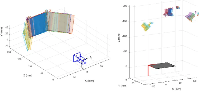
The feasibility of the algorithm’s ability to optically reconstruct the positions was first tested on a literal desktop method with a webcam and pattern. This allowed for a controlled movement of the camera and pattern to confirm the recon. This is shown later in Figure 37 with the maroon vector of the camera coordinate system being the Z axis – the axis perpendicular to the camera lens. The rectangles are the optical pattern positions.
The reconstruction is done using the files discussed in section 3.6 Matlab
Implementation with some slight modifications. For ease of use, here are the files again with the modifications noted:
webcam.m: Found installed with the appropriate webcam drivers on the Applied Nanotechnology group laptop (C:\Users\User\Documents\MATLAB). If installing on another system, the line: handles.vid = videoinput('winvideo', 2, 'RGB24_1920x1080'); should be changed to the appropriate input channel, usually 1 if no other camera drivers are installed (such as a laptop webcam). This opens a GUI that allows the operator to take the images, check to make sure they are of good quality with a zoom ROI feature, retake if necessary, and save into the appropriate folder. Make sure to add the “\” at the end of the folder name. The images are saved numerically. Take an image and save it before every X-ray projection. A screenshot of the GUI is shown in Figure 29.
50
procedure. Returns geo.mat matrix that contains the course data. Check to make sure the values are not (0,0,0). If they are, that means not all of the points were found. Edit the thresholds on line: imfindcircles(image(1:range,1:2560),[10
25],'ObjectPolarity','dark','Sensitivity',0.8,'EdgeThreshold',0.03); OR edits the range parameters ‘p’ added there to help separate the geocal from the actual object. Images 1-10 the geocal is in a certain range but in 11, the object enters that range so from 11-something else, edit the new range to not include the object. Repeat as necessary.
cameraCalibration_DATA_SET_NAME.m: Partially auto-generated by