FLEXIBLE SUPERVISED LEARNING TECHNIQUES WITH APPLICATIONS IN NEUROSCIENCE
Guan Yu
A dissertation submitted to the faculty of the University of North Carolina at Chapel Hill in partial fulfillment of the requirements for the degree of Doctor of
Philosophy in the Department of Statistics and Operations Research.
Chapel Hill 2016
c 2016 Guan Yu
ABSTRACT
Guan Yu: Flexible Supervised Learning Techniques with Applications in Neuroscience
(Under the direction of Yufeng Liu)
ACKNOWLEDGEMENTS
This dissertation would not have been completed without the great support of people who stood by me during my years at UNC. I would like to thank all of them.
TABLE OF CONTENTS
LIST OF TABLES . . . viii
LIST OF FIGURES . . . ix
LIST OF ABBREVIATIONS AND SYMBOLS . . . x
1 INTRODUCTION . . . 1
1.1 Background . . . 1
1.1.1 Penalized Linear Regression . . . 1
1.1.2 Penalized Multivariate Regression . . . 3
1.1.3 Graphical Structure among Predictors . . . 5
1.2 New Contributions and Outline . . . 6
2 SPARSE REGRESSION INCORPORATING GRAPHICAL STRUC-TURE AMONG PREDICTORS . . . 8
2.1 Introduction . . . 8
2.2 Motivation and Methodology . . . 10
2.3 Computation . . . 12
2.3.1 Predictor duplication method . . . 13
2.3.2 Iterative proximal algorithm . . . 13
2.4 Theoretical Properties . . . 17
2.4.1 Subgradient conditions . . . 17
2.4.2 Connections with some existing methods . . . 17
2.4.3 Finite Sample Bounds . . . 18
2.4.4 Asymptotic Normality and Model Selection Consistency . . . 19
2.5.1 Performance Comparison . . . 24
2.5.2 Sensitivity Study . . . 33
2.5.3 PD method v.s. IP algorithm . . . 37
2.6 Real Data Example . . . 39
2.7 Conclusion . . . 42
2.8 Proofs . . . 42
3 GRAPH GUIDED MULTI-TASK LEARNING WITH APPLICATIONS IN NEUROSCIENCE . . . 55
3.1 Introduction . . . 55
3.2 Materials . . . 57
3.2.1 Data . . . 57
3.2.2 Data Preprocessing . . . 58
3.3 Method . . . 59
3.3.1 Notation . . . 59
3.3.2 Extract the correlation information among features . . . 60
3.3.3 Graph Guided Multi-task Learning (GGML) method . . . 61
3.3.4 Computation . . . 64
3.4 Simulation Study . . . 65
3.4.1 Simulated examples . . . 65
3.4.2 Simulation results . . . 66
3.5 Analysis of the ADNI dataset . . . 67
3.5.1 Partial correlation among different features . . . 69
3.5.2 Classification results . . . 69
3.5.3 Regression results . . . 70
3.5.4 Most discriminative brain regions . . . 71
3.6 Discussion . . . 74
3.6.1 Construction of the undirected feature graphG. . . 74
3.7 Conclusion . . . 75
4 SPARSE REGRESSION FOR BLOCK-MISSING MULTI-MODALITY DATA . . . 81
4.1 Introduction . . . 81
4.2 Motivation and Methodology . . . 83
4.3 Simulation Study . . . 87
4.3.1 Simulated examples . . . 87
4.3.2 Simulated results . . . 89
4.4 Real Data Analysis . . . 89
4.5 Conclusion . . . 94
LIST OF TABLES
2.1 Comparison of estimation and prediction (Example 1). . . 26
2.2 Comparison of model selection (Example 1). . . 27
2.3 Comparison of estimation and prediction (Example 2). . . 28
2.4 Comparison of model selection (Example 2). . . 29
2.5 Comparison of estimation and prediction (Example 3). . . 30
2.6 Comparison of model selection (Example 3). . . 31
2.7 Comparison of NMR and ZMR (Sample sizes: 40/40/400). . . 32
2.8 Comparison of NMR and ZMR (Sample sizes: 80/80/400). . . 33
2.9 Comparison of NMR and ZMR (Sample sizes: 120/120/400). . . 34
2.10 Comparison of estimation and prediction (Adjusted Example 2). . . 36
2.11 Comparison of model selection (Adjusted Example 2). . . 37
2.12 Time comparison between PD method and IP algorithm. . . 38
3.1 Demographic information of the 199 subjects used in this study. . . 58
3.2 Comparison of different methods using the simulated examples . . . 76
3.3 Comparison of the classification performance on the ADNI dataset. . . 77
3.4 Comparison of the regression performance on the AD/NC dataset. . . 77
3.5 Comparison of the regression performance on the MCI/NC dataset. . . 78
3.6 Comparison of the top ten selected ROIs for the classification task. . . 78
3.7 Comparison of the top ten selected ROIs for the prediction of MMSE. . . 79
3.8 Comparison of the top ten selected ROIs for the prediction of ADAS. . . 79
3.9 Names of the selected ROIs in this study. . . 80
4.1 Performance comparison of Example 1. . . 90
4.2 Performance comparison of Example 2. . . 91
4.3 Performance comparison of Example 3. . . 93
4.4 Prediction Performance of MMSE score. . . 94
LIST OF FIGURES
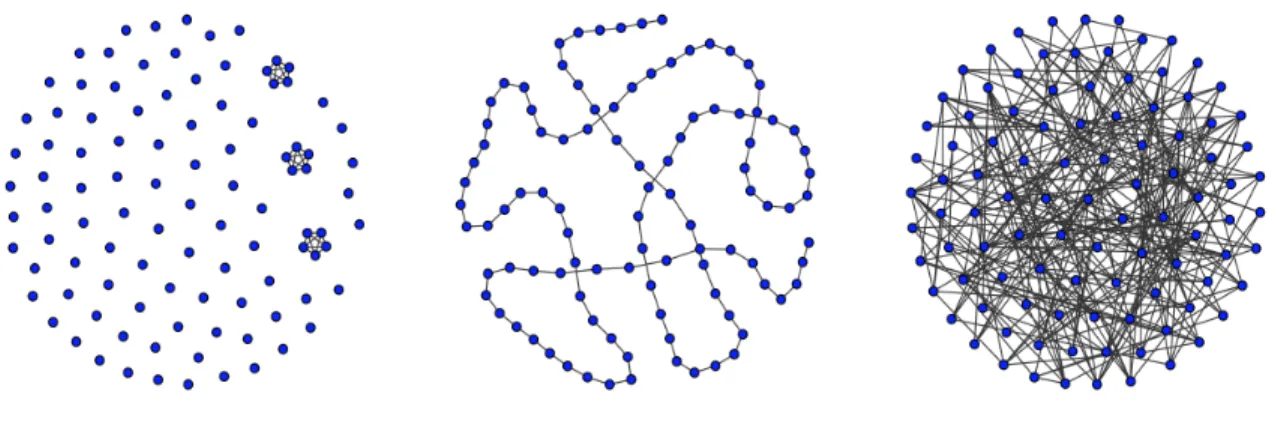
2.1 True predictor graphs of three simulation examples. . . 24
2.2 Sensitivity study of the SRIG method. . . 35
2.3 Estimated graph of 93 MRI features. . . 40
2.4 Comparison of MSE for various methods on the ADNI data set. . . 40
2.5 The multi-slice view of seven brain regions always selected by SRIG method. 41 3.1 Transforming a precision matrix ˆΩ into an undirected graphG. . . 61
3.2 Binary maps of the true precision matrices corresponding to these three simulated examples: Left (Example 1), Middle (Example 2), and Right (Example 3). . . 64
3.3 True feature graphs corresponding to these three simulated exam-ples: Left (Example 1), Middle (Example 2), and Right (Example 3). Each blue dot indicates a feature. . . 66
3.4 Binary maps of the estimated precision matrices. First row: AD/NC data; Second row: MCI/NC data. First column: use only MRI features; Second column: use only PET features; Third col-umn: use both MRI and PET features. . . 67
3.5 Feature graphs corresponding to the estimated precision matrices. First row: AD/NC data; Second row: MCI/NC data. First column: use only MRI features; Second column: use only PET features; Third column: use both MRI and PET features. Each blue dot represents a MRI feature and each green dot represents a PET feature. . . 68
3.6 Selection frequency of 93 ROIs for the AD/NC classification task. . . 71
3.7 Top ten most discriminative brain regions (AD/NC dataset). . . 73
3.8 Top ten most discriminative brain regions (MCI/NC dataset). . . 74
4.1 An illustration of a block-missing multi-modality data set with three modalities. 82 4.2 Selection frequency of 191 features for the prediction of MMSE score. The 93 blue bars represent 93 MRI features, the 93 green bars represent 93 PET features, and the 5 purple bars represent 5 CSF features. . . 92
LIST OF ABBREVIATIONS AND SYMBOLS
AD MCI NC ADNI MRI PET CSF MMSE ADAS-Cog SRIG
Σ
Ω
G
Ni kAk2 kAk∞ kAkF
Alzheimer’s Disease Mild cognitive impairment Normal control
Alzheimer’s Disease Neuroimaging Initiative Structural magnetic resonance imaging
Fluorodeoxyglucose positron emission tomography Cerebrospinal fluid
Mini mental state examination score
Alzheimer’s disease assessment scale-cognitive subscale score
Sparse regression incorporating graphical structure among predictors Population covariance matrix
Population precision matrix Undirected predictor graph The neighborhood of predictori
The`2 norm of the vectorA max1≤i≤k
Pm
j=1|Aij|ifA is ak×m matrix q
Pk i=1
Pm
CHAPTER 1: INTRODUCTION
1.1 Background
Supervised learning techniques play an important role in statistics. Among the existing supervised learning techniques, penalized regression is a very popular one, partly due to its simple formulation and good performance in practice. The basic idea of penalized regres-sion is to perform penalized least squares incorporating some additional constraints on the regression coefficients. In this section, we first briefly review some fundamental penalized regression techniques. In Section 1.1.1, some popular penalized univariate linear regression methods in the literature are reviewed. In Section 1.1.2, we discuss the extension of penal-ized regression methods from univariate regression to multivariate regression. In Section 1.1.3, we discuss how to use an undirected graph to represent the structure information among predictors.
1.1.1 Penalized Linear Regression
Linear regression is a typical supervised learning task and it is commonly used in prac-tice. The model is
Y =Xβ0+, (1.1)
where X ∈Rn×p is the predictor (design) matrix, Y ∈Rn is the response vector,n is the
number of observations,p is the number of predictors,β0= (β10, β02, . . . , βp0)T is a vector of unknown coefficients, and is a vector of independently and identically distributed (i.i.d.) random variables with mean 0 and finite varianceσ2.
often leads to complicate models with low prediction accuracy when the predictors are highly correlated. Furthermore, for the high dimensional data (pn), OLS is not applicable due to the rank deficiency of the design matrix. In order to improve OLS, many penalized methods using regularization in model fitting have been proposed in the literature. The general form of penalized regression is shown as follows:
ˆ
β = arg min
β kY −Xβk 2
2+λP(β),
whereλis a tuning parameter and P(β) is a penalty term that can be used to incorporate all kinds of constraints on the regression coefficients.
Different choices of the penalty termP(β) lead to different penalized regression methods. For example, classical ridge regression ((Hoerl and Kennard, 1970)) uses the ridge penalty
Pp
i=1|βi0|2to possibly achieve better prediction performance through a bias-variance trade-off. The popular Lasso method ((Tibshirani, 1996)) uses thel1penalty
Pp
i=1|βi0|to perform continuous shrinkage and automatic variable selection simultaneously. It is known from the literature that Lasso has many good theoretical properties such as model selection consistency ((Zhao and Yu, 2006)), estimation consistency ((Knight and Fu, 2000)), and persistence property ((Greenshtein, 2006)). However, Lasso also has some limitations. For example, the shrinkage introduced by Lasso results in significant bias towards 0 for large regression coefficients ((Fan and Li, 2001)). In the presence of some highly correlated variables, Lasso tends to select only one of those variables ((Zou and Hastie, 2005)).
convex combination of thel1 and ridge penalty. In the literature, there are also some other important penalized regression methods. For example, (Wang et al., 2007) utilized the least absolute deviation Lasso for robust regression. (Witten and Tibshirani, 2009) proposed the Scout method which includes many penalized methods as special cases.
Although the penalized regression methods introduced above are designed for the uni-variate regression problem, the corresponding regularization ideas are very general and can be also used for multivariate regression. In the next section, we will introduce some penal-ized regression methods for multivariate regression.
1.1.2 Penalized Multivariate Regression
In Section 1.1.1, we have introduced some penalized linear regression methods. In this section, we focus on penalized multivariate regression, which is also called multi-task learning in machine learning if we use linear models to predict multiple correlated continuous response variables. The multivariate regression model is
Y=XB+e, withe= [e1,e1, . . . ,en]T, (1.2)
where Y ∈ Rn×q is the response matrix, B ∈
Rp×q is the coefficient matrix, and
ei = (ei1, ei2, . . . , eiq)T;i = 1,2, . . . , n, are i.i.d. q-dimensional random vectors following a multivariate distribution with mean 0q×1 and covariance matrix ΣY.
Besides the curd and whey method, a lot of further developments have been made in the literature. One popular way to capture the relatedness among multiple response variables is to constrain all regression models to share a common set of predictors (i.e., elements in each row of B are constrained to be zero or nonzero simultaneously). To that end, many existing methods use mixed-norm penalties. Some well known examples of such methods are thel1/l2norm ((Obozinski et al., 2010)) and thel1/l∞norm (Turlach et al., 2005; Zhang et al., 2008). These methods could have good prediction performance and also deliver sparse models for variable selection. The statistical properties of these methods are discussed in (Obozinski et al., 2011b).
Another way to use the correlation information among response variables is to constrain the coefficient matrix B to have a low-rank structure. However, we can not use the rank function as the penalty term directly to constrain the rank of B since the corresponding optimization problem is non-deterministic polynomial-time hard (NP-hard). To solve this issue, (Yuan et al., 2007) uses a new penalty based on the trace norm (also called nuclear norm) of the coefficient matrix B. This penalty encourages the sparsity among singular values and therefore reduces the rank of the estimated coefficient matrix. Moreover, the reduced-rank regression methods (Reinsel and Velu, 1998; Chen and Huang, 2012) can be also used to achieve a low-rank estimation of B. Generally, these methods constrain rank(B) =r for some r ≤min{p, q}. However, as mentioned in (Yuan et al., 2007), since the parameterris often chosen in a separate hypothesis testing or cross validation step, the reduced-rank regression methods can be unstable. Furthermore, although methods encour-aging a low-rank structure of B incorporate the correlation information among responses, most of them do not address the problem of variable selection. In the literature, besides methods using mixed-norm penalties and methods encouraging a low-rank structure of the coefficient matrix, there are also some methods proposed to estimate the coefficient matrix
1.1.3 Graphical Structure among Predictors
Despite the vast literature on penalized methods shown above for univariate regres-sion or multivariate regresregres-sion, few methods directly incorporate the structure/correlation information among predictors efficiently, and at the same time perform simultaneous esti-mation, prediction, and model selection. Typically, the structure/correlation information among predictors can be modeled by the connectivity of an undirected graph. It would be very interesting and useful to study how to use this structure information to improve the performance of variable selection, estimation and prediction.
1.2 New Contributions and Outline
In this dissertation, we investigate some new penalized regression methods for univariate regression and multivariate regression. In addition, we propose a new sparse regression procedure for block-missing multi-modality data. The outline of the dissertation is shown as follows:
• In Chapter 2, we propose a new penalized regression method incorporating the struc-ture/correlation information among predictors directly. Typically, such information can be modeled by the connectivity of an undirected graph using all predictors as nodes of the graph. Our proposed method incorporates this graph information node-by-node by a special latent group Lasso penalty. Theoretical study indicates that our proposed method is very general and it includes adaptive Lasso, group Lasso, and ridge regression as special cases. Furthermore, it acquires tight finite sample bounds for both estimation and prediction, and enjoys model selection consistency for the high dimensional case. Both simulation study and real data analysis demonstrate the effectiveness of the proposed method for simultaneous estimation, prediction and model selection.
• In Chapter 3, we extend the idea of incorporating the structure/correlation informa-tion among predictors to a multi-task learning problem. A new multi-task learning method using both the structure/correlation information among predictors and the correlation information among response variables is proposed. Specifically, based on the undirected predictor graph, our new proposed method encourages the correlated predictors to be in or out of the model together. Furthermore, this new method also encourages the correlated response variables to share a common predictor subset. As a practical application of our new proposed method, a joint prediction of class label and clinical scores of the Alzheimer’s disease using the ADNI data set will be studied in detail.
CHAPTER 2: SPARSE REGRESSION INCORPORATING GRAPHICAL STRUCTURE AMONG PREDICTORS
2.1 Introduction
During the last few decades, despite the vast literature on sparse regression, few methods use the structure information of the predictors which can be modeled by the connectivity of an undirected graph. It would be very interesting and useful to study how to use this structure information to improve the performance of variable selection, estimation and prediction. Since the predictor graph can not be represented as some non-overlapping groups, the traditional group Lasso method ((Yuan and Lin, 2006)) cannot make full use of this complicate structure information. To use the entire predictor graph information, most existing methods use the graph edge-by-edge, through adding some penalty terms to encourage coefficients β0
i and βj0 to be similar for predictors i and j connected by an edge. One type of methods encourages β0i and βj0 to be zero or nonzero simultaneously. For example, OSCAR ((Bondell and Reich, 2008)) uses the l∞ penalty max{|βi0|,|βj0|}for every pair of different predictors. (Yang et al., 2012) generalized OSCAR to graph OSCAR (GOSCAR) which only uses thel∞penalty for those pairs of predictors connected by an edge in the given predictor graph. (Pan et al., 2010) introduced a weighted Lγ-regularization. (Kim et al., 2013) proposed a new non-convex penalty term based on the truncated lasso penalty.
Another type of methods uses some penalty terms to encourageβ0i andβj0 have similar values or absolute values. For example, GRACE ((Li and Li, 2008)) uses the penalty (β0i/√di −βj0/
p
|βi0|and|βj0|to be similar. Although penalized methods using the predictor graph edge-by-edge are promising in improving regression performance, they also have some drawbacks. On the one hand, these methods do not directly utilize the neighborhood information of the graph. For each neighborhood, it can be preferable to use the corresponding edges jointly rather than separately. On the other hand, the penalty terms in these methods will be more complicate if there are more edges in the graph.
In order to make use of the structure information among predictors, instead of using the predictor graphedge-by-edge, we propose a new method, namely Sparse Regression In-corporating Graphical structure among predictors (SRIG), using the graph node-by-node. Specifically, according to the predictor graphG, we assume that there is a latent decompo-sition of β0 intop partsV(1), V(2), . . . , V(p) such that β0 =Pp
i=1V(i) and each V(i) ∈Rp. The proposed SRIG imposes a penalty to shrink someV(i) to 0 while the otherV(i)’s satisfy
supp(V(i)) =Ni, whereNi is a set including predictoriand its neighbors in graphG. For SRIG, if one predictor is important for prediction, the other predictors connected to it are also encouraged to be in the model. Note that our proposed SRIG method is a graph based penalized regression method with a very different motivation, although the corresponding optimization problem can be formulated as a special case of the Latent Group Lasso ap-proach ((Obozinski et al., 2011a)) with each neighborhoodNi as a group. For computation, besides introducing the predictor duplication method shown in (Obozinski et al., 2011a), we also propose a new iterative proximal algorithm which is very efficient for high dimensional data. Our theoretical study shows that SRIG has close connections with several existing methods: (1) It is the same as the adaptive Lasso method when the predictor graph G
features are used to predict the mini-mental state examination (MMSE) score ((Folstein et al., 1975)). Both the simulation results and the real data application indicate that SRIG has competitive performance in estimation, prediction and model selection.
The rest of the chapter is organized as follows. In Section 2.2, we motivate and intro-duce our proposed SRIG method. In Section 2.3, we introintro-duce two methods to solve the optimization problem. In Section 2.4, we show some theoretical properties. In Sections 2.5 and 2.6, we demonstrate the use of SRIG on simulated data and the ADNI dataset. We conclude this chapter with some discussion in Section 2.7. Technical proofs are provided in Section 2.8.
2.2 Motivation and Methodology
Consider the following linear regression model:
Y =Xβ0+, (2.1)
where = (1, 2, . . . , n)T is a vector of i.i.d. random variables with mean 0 and variance
σ2. Here,β0 = (β10, β20, . . . , βp0)T is a vector of true coefficients, Y = (y1, y2, . . . , yn)T is an
n×1 response andX= (X1, X2, . . . , Xp) = (x1, x2, . . . , xn)T is ann×p design matrix. For motivation, we first consider the random design setting and assume that each xk follows some multivariate distribution with mean 0p×1 and covariance matrix Σ. The de-sign matrix X is assumed to be independent of the random error . Furthermore, denote
Ω= (ωij)i,j=1,2,...,p =Σ−1 and Σxy = (c1, c2, . . . , cp)T ∈Rp as the cross-covariance vector betweenxk andyk.
By model (2.1) and the definition of cross-covariance, we have
Σxy =E(XTY /n) =E(XTXβ0/n) +E(XT/n) =Σβ0.
β10=c1ω11+c2ω12+· · ·+ciω1i+· · ·+cpω1p
β20=c1ω21+c2ω22+· · ·+ciω2i+· · ·+cpω2p ..
.
βp0=c1ωp1+c2ωp2+· · ·+ciωpi+· · ·+cpωpp.
As shown in the above equations, β0 is the sum ofp parts, {(ciω1i, ciω2i, . . . , ciωpi)T : 1≤
i≤ p}. For the ith part, (ciω1i, ciω2i, . . . , ciωpi)T, there is a common factor ci. If the ith predictor and the response variable are uncorrelated marginally, then ci will be 0 and all the components in the ith part of β0 will be 0 simultaneously. Furthermore, if ci is not zero and the predictor graph is defined by Ω, then the support of (ciω1i, ciω2i, . . . , ciωpi)T becomes Ni, which is a set including predictor iand its neighbors in the predictor graph. Thus, instead of focusing on β0 in the model, we consider a latent decomposition of β0
into p parts. After choosing the candidate non-zero components in each part based on N1,N2, . . . ,Np, we use the group lasso penalty to encourage the selected components in each part to be zero or nonzero simultaneously.
The above idea can be generalized for an arbitrary predictor graph constructed by the prior information or estimation from data. Given the predictor graph G, we define a
p×p adjacency matrix E, whereEij = 1 if predictors i and j are connected and Eij = 0 otherwise. For eachi, we set Eii= 1 and acquire the neighborhood setNi ={j:Eij = 1}. As the previous case, we assume that β0 can be decomposed into
β10=V1(1)E11+V1(2)E12+· · ·+V1(i)E1i+· · ·+V1(p)E1p
β20=V2(1)E21+V2(2)E22+· · ·+V2(i)E2i+· · ·+V2(p)E2p ..
.
βp0=Vp(1)Ep1+Vp(2)Ep2+· · ·+Vp(i)Epi+· · ·+Vp(p)Epp.
Vj(i)will be zero for eachj∈ Niand the components in the set{Vj(i)Eji:j∈ Ni}will be zero simultaneously. Therefore, after choosing the candidate non-zero components in each part based on N1,N2, . . . ,Np, it is reasonable to use the group lasso penalty to encourage the selected components in each part to be zero or nonzero together. Based on this motivating idea, given the training data (Y,X) and the predictor graphG, we propose a new method, Sparse Regression Incorporating Graphical structure among predictors (SRIG), shown as follows.
SRIG Method
Step 1: Find the neighborhoodsN1,N2, . . . ,Np (note thati∈ Ni for each i).
Step 2: Solve the following optimization problem:
min β,V(1),...,V(p)
1
2nkY −Xβk
2 2+λ
p X
i=1
τikV(i)k2, (2.2)
subject to Pp
i=1V(i) =β and supp(V(i))⊆ Ni for each i, where supp(V(i)) is the support of vectorV(i) and k · k2 is the l2 norm.
Here,τidenotes the positive weight for thei-th group. The choice ofτiwill be discussed in Section 2.4.4.
2.3 Computation
2.3.1 Predictor duplication method
DenoteVN(i)
i as the|Ni| ×1 sub-vector ofV
(i)with indices inN
iandXNi as then× |Ni|
sub-matrix of X with column indices in Ni. Denote ˜V = (V(1)
T
N1 , V
(2)T
N2 , . . . , V
(p)T
Np )
T and ˜
X = (XN1, XN2, . . . , XNp). Then, we can check that Xβ = ˜XV˜, and problem (2.2) is
equivalent to the following group Lasso problem:
min ˜ V
1
2nkY −X˜V˜k
2 2+λ
p X
i=1
τikVN(i)ik2 (2.3)
Many efficient R packages such as grpreg ((Breheny and Huang, 2009)) and gglasso
((Yang and Zou, 2013)) can be used to solve problem (2.3). After setting ˆVN(i)c
i = 0 for eachi,
we have ˆβ =Pp
i=1Vˆ(i). Note that in some cases, some neighborhoods {Ni :i∈F} maybe exactly the same. Then, the vectors {VN(i)
i :i∈F} are indistinguishable and therefore the
decomposition of β (i.e., {V(1), V(2), . . . , V(p)}) is not unique. In this case, although we can not estimate each vector in {VN(i)
i :i ∈F} stably, we can estimate
P i∈F V
(i)
Ni directly
and stably using the penalty term (mini∈Fτi)kPi∈FV (i)
Nik2. Since ˆβ=
Pp
i=1Vˆ(i), different decompositions of β lead to the same estimation of β.
The predictor duplication method shown above is very convenient to use and has good performance in general. However, when the dimensional is high and at the same time the predictor graph is not very sparse, there will be a lot of duplicated predictors in (2.3) and therefore the predictor duplication method can be inefficient ((Obozinski et al., 2011a)). In the following Section 2.3.2, we will propose a new iterative proximal algorithm which does not duplicate predictors. It is stable and very efficient for the high dimensional data, espe-cially when the predictor graph can be decomposed into several disconnected components.
2.3.2 Iterative proximal algorithm
Given the predictor graphG and positive weightsτi’s, forβ ∈Rp, define
kβkG,τ =Pp min
i=1V(i)=β, supp(V(i))⊆Ni
p X
i=1
We can show thatkβkG,τ is a norm ((Obozinski et al., 2011a)) and (2.2) is equivalent to
min β∈Rp
1
2nkY −Xβk
2
2+λkβkG,τ (2.5)
In problem (2.5), the squared loss function is strictly convex and differentiable. In addition, kβkG,τ is a norm and therefore convex. Thus, we can use the Fast Iterative Shrinkage Thresholding Algorithm (FISTA) ((Beck and Teboulle, 2009)) to solve it. For our specific problem (2.5), we propose the following iterative proximal algorithm.
Iterative Proximal (IP) Algorithm
Input: The initial estimate β(0) and L= the largest eigenvalue ofXTX/n.
Step 0: Take Z(1)=β(0)∈Rp and t1= 1.
Step m: (m≥1) Compute
β(m)= arg min
β λkβkG,τ+
L
2kβ−(Z
(m)− 1
nLX
T(XZ(m)−Y))k2
2, (2.6)
tm+1=
1 +p1 + 4t2 m
2 ; Z
(m+1)=β(m)+tm−1
tm+1
(β(m)−β(m−1)).
By Theorem 4.4 in (Beck and Teboulle, 2009), the sequences{β(m)}generated via (2.6) will converge to the optimal solution with rateO(1/m2). The most time consuming step in the above IP algorithm is to compute the proximal operator ofλkβkG,τ, which is defined as
proxλkβkG,τ(h) = arg minβ λkβkG,τ +
kβ−hk2 2
2 . (2.7)
Follow the same proofs of Lemmas 1 and 2 in (Villa et al., 2014), we can show that
proxλkβk
G,τ(h) =h−arg minβ∈S
O
kβ−hk2, (2.8)
In (2.8), we need to solve the following optimization problem
u∗= arg min β∈SO
kβ−hk2
Based on the number of elements in O, denoted asM =|O|, we use different methods flexibly to find the projection of h onto the convex set SO efficiently. If |O|is small (e.g., smaller thanp/10 in our simulation study), we calculate the projection by solving the dual problem via the Bertsekas’s projected Newton method ((Villa et al., 2014)). The solution is
u∗j = hj 1 +P
i∈Ot∗i1i,j
, forj= 1,2, . . . , p,
wheret∗ is the solution of
arg max t∈RM +
f(t), withf(t) = p X
j=1
−h2j
1 +P
i∈Oti1i,j
−X
i∈O
tiλ2τi2
L2 ,
and 1i,j equal to 1 ifj belong to Ni and 0 otherwise. The detailed algorithm to solve the above dual problem is shown in Algorithm 5 in (Villa et al., 2014).
If|O|is large (e.g., larger thanp/10), we propose to find the projection by the Parallel Dykstra-like proximal algorithm ((Combettes and Pesquet, 2011)). The detailed algorithm is shown as follows.
Parallel Dykstra-like proximal algorithm
Step n: (n≥1) Compute
pi,nNc i =z
i,n Nc
i for each i∈ O; pi,nN
i =z
i,n Ni1(kz
i,n Nik ≤
λτi
L ) +
λτizi,nNi
Lkzi,nN ik2
1(kzNi,n ik>
λτi
L ) for each i∈ O;
u(n+1)=X i∈O
p(i,n)
M ;
zi,n+1=u(n+1)+zi,n−pi,n for each i∈ O.
The sequence {u(n)} will converge to the projection of h onto S O.
Furthermore, we note that the proposed IP algorithm is scalable to large scale prob-lems when the predictor graph G can be decomposed into several components (i.e., the covariance/precision matrix is block diagonal). Denote the disconnected components in G
asG1, G2, . . . , GK with node setsC1,C2, . . . ,CK, respectively. In this case, we can compute the proximal operator (2.7) efficiently by solving the followingK subproblems in parallel:
proxλkβC
kkGk,τCk(hCk) = arg minβC
k
λkβCkkGk,τCk +
kβCk −hCkk
2 2
2 ,
whereβCk,τCk,hCk are sub-vectors ofβ,τ, and h, respectively.
2.4 Theoretical Properties
In this section, we study the theoretical properties of our proposed SRIG method. For theoretical study, it is convenient to consider (2.5) as the objective function. In (2.5), the optimal decomposition of β minimizing kβkG,τ always exists, but may not be unique ((Obozinski et al., 2011a)). DenoteJ0={i:βi0 6= 0},J0c={i:βi0= 0}, ands0=|J0|as the true nonzero coefficient set, the true zero coefficient set, and the number of true nonzero co-efficients, respectively. For eachβ ∈Rp, denoteU(β) as the set of all optimal decompositions ofβ, andKG,τ(β) as the number of nonzeroV(i)’s in the optimal decomposition ofβ which has the minimal number of nonzero V(i)’s, i.e., KG,τ(β) = min(V(1),V(2),...,V(p))∈U(β)|{i :
kV(i)k2 6= 0}|. Denote KG,τ = supsupp(β)⊆J0KG,τ(β). We can check that KG,τ = s0 if the
graph G has no edge, KG,τ = K0 if G consists of some disconnected complete subgraphs and J0 is the union of K0 node sets of those disconnected subgraphs.
2.4.1 Subgradient conditions
The following proposition shows the subgradient conditions for problem (2.5).
Proposition 1. A vectorβ ∈Rp is a solution of (2.5) if and only ifβ can be decomposed asβ =Pp
i=1V(i)whereV(i)’s satisfy that, for all 1≤i≤p, (a)V (i) Nc
i = 0; (b) eitherV
(i) Ni 6= 0
and XNT
i(Y −Xβ) =nλτi
VN(i)
i
kVN(i)
ik2
, orVN(i)
i = 0 andkX
T
Ni(Y −Xβ)k2 ≤nλτi.
The subgradient conditions shown above are similar to the subgradient conditions for the latent group Lasso ((Obozinski et al., 2011a)) and group Lasso ((Nardi and Rinaldo, 2008)). According to Proposition 1, if ( ˆV(1),Vˆ(2), . . . ,Vˆ(p)) is a solution of problem (2.2), then for each i, either ˆV(i) = 0p×1 or supp( ˆV(i)) = Ni. Thus, the estimate ˆβ = Ppi=1Vˆ(i) acquired by our proposed SRIG method has the same decomposition pattern as we discussed in Section 2.2.
2.4.2 Connections with some existing methods
Proposition 2. (a) If the predictor graph has no edge, the proposed SRIG method is the same as the adaptive Lasso method for each tuning parameterλ; (b) If the predictor graph consists of K disconnected complete subgraphs, our proposed SRIG method is equivalent to the group Lasso method for each λ; (c) If the predictor graph is a complete graph, our proposed SRIG method has the same nonzero solution set as the ridge regression, i.e., for each nonzero solution acquired by ridge regression (or SRIG), SRIG (or ridge regression) could acquire the same solution using a different tuning parameter.
Proposition 2 indicates that the proposed SRIG method includes adaptive Lasso, group Lasso, and ridge regression as special cases. It is much more general and can handle any arbitrary predictor graph structure.
2.4.3 Finite Sample Bounds
In this section, we derive the oracle inequalities for the prediction and estimation loss of our proposed SRIG method. The design matrixX is treated as fixed in this subsection. For a given graphG, positive weightsτj’s and subset J ⊂ {1,2. . . , p}, denoteTG,τ(β, J) as the set of all optimal decompositions of β such that P
j∈JcτjkV(j)k2 ≤ 3Pj∈JτjkV(j)k2. For each 1 ≤ i ≤ p, denote di as the number of predictors in the neighborhood Ni, i.e.,
di=|Ni|. The following conditions are considered in this section.
(A1) The errors 1, 2, . . . , ni.i.d.∼ N(0, σ2).
(A2) The neighborhood Ni ⊆J0 for each i∈J0.
(A3) There exists κ >0 such that
inf |J|≤s0,β∈Rp\{0}
inf (V(1),V(2),...,V(p))∈T
G,τ(β,J)
kXβk2 q
nP
j∈Jτj2kV(j)k22 ≥κ.
overlapped group Lasso ((Percival, 2012)). It is used to analyze thel2 consistency property of both estimation and prediction.
Theorem 1. Suppose that conditions (A1), (A2) and (A3) are satisfied. Let τ∗ = min1≤i≤pτi and denoteηi as the positive square root of the largest eigenvalue of n1XNTiXNi.
If we choose λτi ≥ 2ση√ni(di+Ad1/2i log(p))1/2 whereA >8, then, for any optimal solution ˆβ of problem (2.5), we have
1
nkX( ˆβ−β
0)k2 2 ≤
16λ2K G,τ
κ2 ,
kβˆ−β0kG,τ ≤ 16λKG,τ
κ2 , kβˆ−β0k2 ≤ 16λKG,τ
κ2τ∗ ,
with probability at least 1−p1−q, whereq= 81min{A, A2log(p)}.
Remark 1. Note that the above results are very general and have close connections with the results shown in the literature. For example, when the predictor graphG has no edge, we haveKG,τ =s0 and kβˆ−β0kG,τ =kβˆ−β0k1 if τi = 1 for each i. Theorem 1 indicates that our proposed SRIG method acquires the same rates of prediction and estimation as the results shown in (Bickel et al., 2009) for the Lasso method. When the given graph G
consists of some disconnected complete subgraphs and J0 is the union ofK0 node sets of those disconnected subgraphs, we have KG,τ = K0. In this case, we can also recover the results shown in (Nardi and Rinaldo, 2008) and (Lounici et al., 2011) for the group Lasso.
2.4.4 Asymptotic Normality and Model Selection Consistency
In this section, we first study the asymptotic normality for the case with a fixed dimen-sionp. Then, we study the model selection consistency for the high dimensional case which allows p to grow withn. Both fixed design and random design are considered in these two cases. For everyβ ∈Rp, denoteβJ0 and βJ0c as the sub-vectors of β with indices inJ0 and
J0crespectively.
(A4) As n→ ∞,XTX/n→ M, whereMis a positive matrix.
(A5) The errors 1, . . . , n are i.i.d. random variables with mean 0 and finite variance σ2.
Theorem 2. Assume conditions (A2), (A4) and (A5) hold. Suppose the tuning parameter
λ and weights τi’s are chosen such that √
nλ → 0 and n(γ+1)/2λ → ∞ for some γ > 0. Furthermore,τj =O(1) for eachj∈J0 and lim infn→∞n−γ/2τj >0 for eachj∈J0c. Then, with dimension pfixed, as n→ ∞, we have
√
n( ˆβJ0−β
0 J0)
d
−→N(0, σ2M−J1
0,J0), and ˆβJ0c
p −→0,
whereMJ0,J0 is the sub-matrix ofMconsisting of the entries with row and column indices
inJ0.
Remark 2. Theorem 2 indicates that our proposed SRIG method is estimation-consistent for the fixedpcase. The estimates of the nonzero coefficients enjoy the asymptotic normality. Theorem 2 also provides a guideline on how to choose the positive weightτj. When n > p, similar to the weights used for the Adaptive Lasso ((Zou, 2006)), we can choose τj = p
dj/|βˆjγ|, where ˆβj is any √
n-consistent estimate of βj0. Note that Theorem 2 can be extended to the random design setting naturally.
Corollary 1. Consider the random design setting where x1, x2, . . . , xn are i.i.d. samples from a multivariate distribution with mean 0 and covariance matrix Σ. Assume that the design matrixXand the errorsare independent. Suppose conditions (A2) and (A5) hold. The tuning parameterλand weightsτi’s are chosen such that
√
nλ→0 andn(γ+1)/2λ→ ∞ for some γ > 0. Furthermore, τj = O(1) for each j ∈ J0 and lim infn→∞n−γ/2τj > 0 for each j∈J0c. Then, with pfixed, as n→ ∞, we have
√
n( ˆβJ0 −β
0 J0)
d
−→N(0, σ2Σ−J1
0,J0), and ˆβJ0c
p −→0,
where ΣJ0,J0 is the sub-matrix of Σ consisting of the entries with row and column indices
For the high dimensional case which allows the dimension p to grow with n, if the design matrix X is considered to be fixed, we need the following conditions for model selection consistency.
(A6) The number of nonzero coefficients s0=O(nδ0) for some constant δ0∈(0,1).
(A7) There exists a constant Q1>0 such that maxj∈Jc
0kXjk2 ≤
√
nQ1 for each n.
(A8) There exists a constant Q2 > 0 such that the smallest eigenvalue of XJT0XJ0/n is
larger than Q2 for each n.
(A9) There exists a constant ξ ∈(0,1) such that kXJTc 0XJ0(X
T J0XJ0)
−1k
∞ ≤1−ξ, where for a k×mmatrix M,kMk∞ is defined as max1≤i≤kPmj=1|Mij|.
Note that condition (A6) is a common sparsity assumption for the high dimensional regression problem. Condition (A7) can be satisfied by normalizing each predictor. Condi-tion (A8) guarantees that the matrix XJT
0XJ0/n is invertible and its inverse behaves well.
The main condition (A9) is similar to the strong irrepresentable condition used for Lasso ((Zhao and Yu, 2006)).
Theorem 3. Assume conditions (A1), (A2), (A6)-(A9) hold. Suppose the weight τj is chosen to be p
djmj for each j, where the mj’s satisfy that maxj∈J0mj = Op(1) and
lim infn→∞n−γminj∈Jc
0mj >0 for some γ > δ0. Furthermore, the selected tuning
param-eter λ and the minimum absolute nonzero coefficient βmin0 = minj∈J0|β
0
j| satisfy that, as
n−→ ∞ and p=p(n)−→ ∞,
1
λ
r
log (p−s0)
n maxj∈Jc 0
p
dj
τj
−→0, and 1
β0 min
(3σ
s
logs0
nQ2 +λ √ s0 Q2 max
j∈J0
τj)−→0.
Then, as n −→ ∞ and p = p(n) −→ ∞, there exists a solution ˆβ to (2.5) such that sign( ˆβ)=sign(β0) with probability tending to 1, where sign(·) maps a positive entry to 1, a negative entry to−1 and zero to zero.
proposed SRIG method is model selection consistent for the high dimensional case. For example, suppose the dimension p = O(enδ1
) for some constant δ1 ∈(0,1). Furthermore, for sufficiently largen, the minimum absolute nonzero coefficientβmin0 satisfies thatβmin0 ≥
Q3n(δ2−1)/2 for some constants Q3 > 0 and δ2 > δ1. If the weights τj’s are selected as shown in the theorem and the tuning parameter λ is chosen to be λ= Op(n(δ1−2δ0−1)/2), then by Theorem 3 we can show that there exists a solution ˆβ such that sign( ˆβ)=sign(β0) with probability tending to 1. In the high dimensional case with p n, our simulation study suggests that choosing τj =
p
dj/|covˆ (Xj, Y)|γ works well. The positive parameter
γ can be chosen by cross-validation.
In Theorem 3, as the Lasso method, we use the irrepresentable condition (A9). In fact, we can also use the following condition (A90) in order to reflect the use of the weights τj’s. Following the same proof of Theorem 3, we can achieve the model selection consistency as shown in Corollary 2.
(A90) There exists a constantξ∈(0,1) such that for eachj∈J0c, we have
kXNTjXJ0(X
T J0XJ0)
−1k ∞≤
τj p
dj
(1−ξ).
Corollary 2. Assume conditions (A1), (A2), (A6)-(A8), (A90) hold. Suppose the weight
τj’s satisfy that √
s0maxj∈J0τj =op(1). Furthermore, the selected tuning parameterλand
the minimum absolute nonzero coefficient βmin0 = minj∈J0|β
0
j|satisfy the same conditions in Theorem 3, then, as n −→ ∞ and p = p(n) −→ ∞, there exists a solution ˆβ to (2.5) such that sign( ˆβ)=sign(β0) with probability tending to 1.
Theorem 3 considers the fixed design setting. It can be extended to the random design setting as well. For that setting, the conditions (A6)-(A9) are replaced by the following conditions.
(A10) Let x1, x2, . . . , xn i.i.d.
∼ N(0,Σ) with Σjj = 1 for eachj. Furthermore, assume that
(A11) Restricted eigenvalue assumption:
Λmin(s0) = 16
17J⊆{1,2,...,pmin},|J|≤s0
min θ6=0, θJ c=0
θTΣθ kθJk22
>0.
(A12) The number of true nonzero coefficientss0<(Λmin(s0)/(16Q3)) p
n/logp.
Note that conditions (A10)-(A12) are common conditions used in the literature for the random design setting ((Bickel et al., 2009; Zhou et al., 2009)). Under these conditions, we can show that our proposed SRIG method is also model selection consistent for the high dimensional case with random design.
Theorem 4. Assume conditions (A1), (A2), (A10)-(A12) hold. Suppose the weight
τj is chosen to be p
djmj for each j, where s3/20 maxj∈J0mj = o(
p
Λmin(s0) minj∈J0cmj).
Furthermore, the selected tuning parameterλand the minimum absolute nonzero coefficient
βmin0 = minj∈J0|β
0
j|satisfy that, asn−→ ∞and p=p(n)−→ ∞,
1
λ
r
log (p−s0)
n maxj∈Jc 0
p
dj
τj
−→0, 1 βmin0 (3σ
s
logs0
nΛmin(s0) +λ
√
s0 Λmin(s0)
max j∈J0
τj)−→0.
Then, as n −→ ∞ and p = p(n) −→ ∞, there exists a solution ˆβ to (2.5) such that sign( ˆβ)=sign(β0) with probability tending to 1, where sign(·) maps a positive entry to 1, a negative entry to−1 and zero to zero.
Remark 4. Under conditions (A10)-(A12), we can show that condition (A7) is satisfied with Q1 =
p
3/2, condition (A8) is satisfied with Q2 = Λmin(s0), and kXT
Jc 0XJ0(X
T J0XJ0)
−1k ∞≤
p
3s0/(2Λmin(s0)), with probability greater than 1−1/p2. Based on these results, we can use a similar proof of Theorem 3 to prove Theorem 4.
2.5 Simulation Study
2.5.1 Performance Comparison
To examine the performance of SRIG, we compare it with many other methods on three examples. Firstly, we compare SRIG with popular penalized methods such as Lasso, Ridge regression, Adaptive Lasso (ALasso) and Elastic net (Enet) which do not use the predictor graph structure information directly. Secondly, we compare SRIG with some existing methods using the predictor structure information. The competitors are GRACE ((Li and Li, 2008)) and GOSCAR ((Yang et al., 2012)). Thirdly, we compare SRIG with other latent component approaches such as principal component regression (PCR) and sparse partial least squares (SPLS) using the R packagespls((Mevik and Wehrens, 2007)) and spls((Chung et al., 2012)), respectively. In this simulation study, the predictor graph is defined by the precision matrix of the predictors. The performance of GRACE, GOSCAR and SRIG using both the estimated predictor graph and the oracle true predictor graph are evaluated on all examples. We denote GRACE-O, GOSCAR-O and SRIG-O as the GRACE, GOSCAR and SRIG methods using the true predictor graph, respectively. For comparison, we also show the performance of the least square method based on the true model, which is denoted as LS-O.
Figure 2.1: True predictor graphs of three simulation examples.
We generate data from model (2.1) with the errors1, 2, . . . , n i.i.d.
are used to choose the tuning parameter and the test data set is used to evaluate different methods. We use the notation ./././ to show the sample sizes in the training, validation and test sets, respectively. For each example, we consider three cases: (I) 40/40/400, (II) 80/80/400 and (III) 120/120/400. For each case, we repeat the simulation 50 times. The predictor graph is estimated by the graphical Lasso method ((Friedman et al., 2008)) only using the training data in all cases.
Example 1: (Ω is block diagonal) p = 100, s0 = 15, σ = 5, and the true coefficient vectorβ0 = (3,3,· · · ,3,0,0,· · ·,0). The predictors are generated as:
Xj =Z1+ 0.4xj, Z1 ∼N(0,1), 1≤j≤5;
Xj =Z2+ 0.4xj, Z2 ∼N(0,1), 6≤j≤10,
Xj =Z3+ 0.4xj, Z3 ∼N(0,1), 11≤j≤15; Xj i.i.d
∼ N(0,1), 16≤j≤100,
wherexj i.i.d∼ N(0,1), j = 1,2, . . . ,15.
Example 2: (Ω is banded) p = 100, σ = 10, and β0 is the same as the β0 used in Example 1. The predictors (X1, X2, . . . , Xp)T ∼N(0,Σ) with Σij = 0.5|i−j|. For this example, we haveωii= 1.333, ωij =−0.667 if|i−j|= 1 and ωij = 0 if |i−j|>1.
Example 3: (Ω is sparse) p = 100, σ = 5, and the predictors (X1, X2, . . . , Xp)T ∼
N(0,Ω−1), whereΩ=L+δI. Each off-diagonal entry inLis generated independently and equals to 0.5 with probability 0.05, or 0 with probability 0.95. The diagonal en-try of L is 0. Here, δ is chosen such that the conditional number of Ω is equal to
p. Finally, Ω is standardized to have unit diagonals. We set β0 = ΩΣxy, where Σxy = (c1, c2, . . . , cp)T with ci = 10 for the predictors having the top four largest degrees andci = 0 otherwise.
To evaluate different methods, we use the following measures:
• l2 distance kβˆ−β0k2;
• False positive rate (FPR) and False negative rate (FNR);
• Nonzero match ratio (NMR) = |{(i,j): Ωij6=0, βˆi6=0, βˆj6=0}|
|{(i,j): Ωij6=0, βi06=0, βj06=0}|
, which is used to check whether the estimated coefficients of two connected useful predictors are both nonzero; Zero match ratio (ZMR) = |{(i,j): Ωij6=0, βˆi=0, βˆj=0}|
|{(i,j): Ωij6=0, β0i=0, β0j=0}|
, which is used to check whether the estimated coefficients of two connected useless predictors are both zero. We use NMR and ZMR when there is at least one edge connecting two useful predictors and one edge connecting two useless predictors. Thus, these two ratios are well defined and always between 0 and 1.
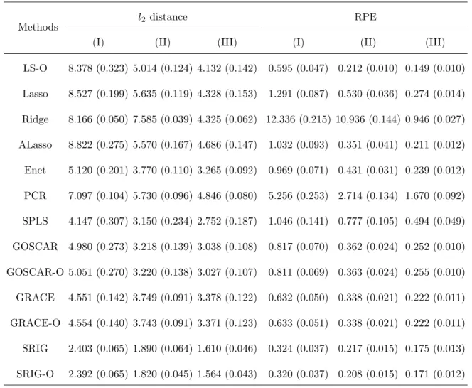
Table 2.1: Comparison of estimation and prediction (Example 1).
Methods
l2 distance RPE
(I) (II) (III) (I) (II) (III)
LS-O 8.378 (0.323) 5.014 (0.124) 4.132 (0.142) 0.595 (0.047) 0.212 (0.010) 0.149 (0.010)
Lasso 8.527 (0.199) 5.635 (0.119) 4.328 (0.153) 1.291 (0.087) 0.530 (0.036) 0.274 (0.014)
Ridge 8.166 (0.050) 7.585 (0.039) 4.325 (0.062) 12.336 (0.215) 10.936 (0.144) 0.946 (0.027)
ALasso 8.822 (0.275) 5.570 (0.167) 4.686 (0.147) 1.032 (0.093) 0.351 (0.041) 0.211 (0.012)
Enet 5.120 (0.201) 3.770 (0.110) 3.265 (0.092) 0.969 (0.071) 0.431 (0.031) 0.239 (0.012)
PCR 7.097 (0.104) 5.730 (0.096) 4.846 (0.080) 5.256 (0.253) 2.714 (0.134) 1.670 (0.092)
SPLS 4.147 (0.307) 3.150 (0.234) 2.752 (0.187) 1.046 (0.141) 0.777 (0.105) 0.494 (0.049)
GOSCAR 4.980 (0.273) 3.218 (0.139) 3.038 (0.108) 0.817 (0.070) 0.362 (0.024) 0.252 (0.010)
GOSCAR-O 5.051 (0.270) 3.220 (0.138) 3.027 (0.107) 0.811 (0.069) 0.363 (0.024) 0.255 (0.010)
GRACE 4.551 (0.142) 3.749 (0.091) 3.378 (0.122) 0.632 (0.050) 0.338 (0.021) 0.222 (0.011)
GRACE-O 4.554 (0.140) 3.743 (0.091) 3.371 (0.123) 0.633 (0.051) 0.338 (0.021) 0.222 (0.011)
SRIG 2.403 (0.065) 1.890 (0.064) 1.610 (0.046) 0.324 (0.037) 0.217 (0.015) 0.175 (0.013)
Table 2.2: Comparison of model selection (Example 1).
Methods
FPR FNR
(I) (II) (III) (I) (II) (III)
LS-O 0.000 (0.000) 0.000 (0.000) 0.000 (0.000) 0.000 (0.000) 0.000 (0.000) 0.000 (0.000)
Lasso 0.087 (0.009) 0.145 (0.014) 0.123 (0.010) 0.171 (0.012) 0.027 (0.005) 0.003 (0.002)
Ridge 1.000 (0.000) 1.000 (0.000) 1.000 (0.000) 0.000 (0.000) 0.000 (0.000) 0.000 (0.000)
ALasso 0.039 (0.007) 0.027 (0.006) 0.041 (0.005) 0.173 (0.016) 0.021 (0.006) 0.007 (0.003)
Enet 0.131 (0.013) 0.171 (0.012) 0.148 (0.013) 0.032 (0.010) 0.000 (0.000) 0.000 (0.000)
PCR 1.000 (0.000) 1.000 (0.000) 1.000 (0.000) 0.000 (0.000) 0.000 (0.000) 0.000 (0.000)
SPLS 0.140 (0.034) 0.274 (0.043) 0.245 (0.034) 0.043 (0.011) 0.004 (0.002) 0.003 (0.002)
GOSCAR 0.190 (0.025) 0.226 (0.007) 0.307 (0.009) 0.039 (0.011) 0.003 (0.002) 0.000 (0.000)
GOSCAR-O 0.230 (0.032) 0.228 (0.007) 0.310 (0.009) 0.036 (0.011) 0.003 (0.002) 0.000 (0.000)
GRACE 0.136 (0.011) 0.135 (0.009) 0.127 (0.011) 0.005 (0.004) 0.000 (0.000) 0.000 (0.000)
GRACE-O 0.138 (0.011) 0.134 (0.009) 0.127 (0.011) 0.005 (0.004) 0.000 (0.000) 0.000 (0.000)
SRIG 0.001 (0.001) 0.003 (0.001) 0.003 (0.001) 0.000 (0.000) 0.000 (0.000) 0.000 (0.000)
SRIG-O 0.000 (0.000) 0.000 (0.000) 0.000 (0.000) 0.000 (0.000) 0.000 (0.000) 0.000 (0.000)
directly. However, Elastic net, GOSCAR and GRACE methods still have relatively high FPR. Compared with the other methods (not including methods using the true predictor graph), our proposed SRIG method delivers the best performance of estimation and predic-tion. Furthermore, SRIG almost always identifies the true model perfectly for this example. Since the estimated predictor graph for this example is almost the same as the true pre-dictor graph, the performance of GOSCAR-O, GRACE-O and SRIG-O are similar to those of GOSCAR, GRACE and SRIG respectively. Due to the strong correlation between dif-ferent important predictors, the performance of LS-O method on this example is not very good. Compared with LS-O, our proposed SRIG method still acquires better performance of estimation and competitive results for prediction.
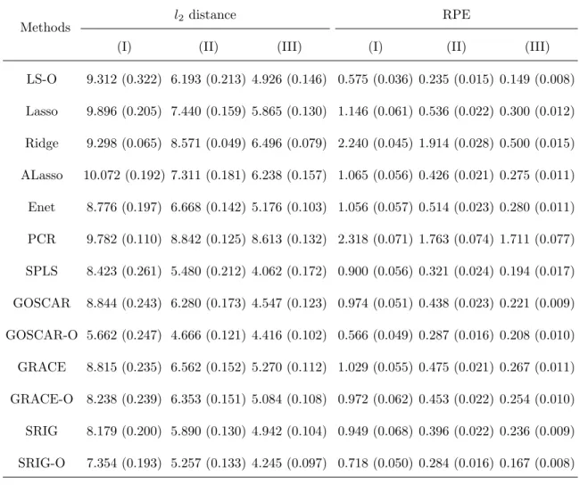
Table 2.3: Comparison of estimation and prediction (Example 2).
Methods
l2 distance RPE
(I) (II) (III) (I) (II) (III)
LS-O 9.312 (0.322) 6.193 (0.213) 4.926 (0.146) 0.575 (0.036) 0.235 (0.015) 0.149 (0.008)
Lasso 9.896 (0.205) 7.440 (0.159) 5.865 (0.130) 1.146 (0.061) 0.536 (0.022) 0.300 (0.012)
Ridge 9.298 (0.065) 8.571 (0.049) 6.496 (0.079) 2.240 (0.045) 1.914 (0.028) 0.500 (0.015)
ALasso 10.072 (0.192) 7.311 (0.181) 6.238 (0.157) 1.065 (0.056) 0.426 (0.021) 0.275 (0.011)
Enet 8.776 (0.197) 6.668 (0.142) 5.176 (0.103) 1.056 (0.057) 0.514 (0.023) 0.280 (0.011)
PCR 9.782 (0.110) 8.842 (0.125) 8.613 (0.132) 2.318 (0.071) 1.763 (0.074) 1.711 (0.077)
SPLS 8.423 (0.261) 5.480 (0.212) 4.062 (0.172) 0.900 (0.056) 0.321 (0.024) 0.194 (0.017)
GOSCAR 8.844 (0.243) 6.280 (0.173) 4.547 (0.123) 0.974 (0.051) 0.438 (0.023) 0.221 (0.009)
GOSCAR-O 5.662 (0.247) 4.666 (0.121) 4.416 (0.102) 0.566 (0.049) 0.287 (0.016) 0.208 (0.010)
GRACE 8.815 (0.235) 6.562 (0.152) 5.270 (0.112) 1.029 (0.055) 0.475 (0.021) 0.267 (0.011)
GRACE-O 8.238 (0.239) 6.353 (0.151) 5.084 (0.108) 0.972 (0.062) 0.453 (0.022) 0.254 (0.010)
SRIG 8.179 (0.200) 5.890 (0.130) 4.942 (0.104) 0.949 (0.068) 0.396 (0.022) 0.236 (0.009)
Table 2.4: Comparison of model selection (Example 2).
Methods
FPR FNR
(I) (II) (III) (I) (II) (III)
LS-O 0.000 (0.000) 0.000 (0.000) 0.000 (0.000) 0.000 (0.000) 0.000 (0.000) 0.000 (0.000)
Lasso 0.154 (0.010) 0.171 (0.014) 0.158 (0.011) 0.304 (0.016) 0.099 (0.010) 0.025 (0.005)
Ridge 1.000 (0.000) 1.000 (0.000) 1.000 (0.000) 0.000 (0.000) 0.000 (0.000) 0.000 (0.000)
ALasso 0.121 (0.012) 0.071 (0.010) 0.081 (0.007) 0.303 (0.018) 0.121 (0.014) 0.052 (0.009)
Enet 0.311 (0.032) 0.273 (0.024) 0.223 (0.016) 0.168 (0.019) 0.051 (0.009) 0.005 (0.003)
PCR 1.000 (0.000) 1.000 (0.000) 1.000 (0.000) 0.000 (0.000) 0.000 (0.000) 0.000 (0.000)
SPLS 0.196 (0.030) 0.050 (0.011) 0.059 (0.021) 0.181 (0.021) 0.096 (0.013) 0.043 (0.007)
GOSCAR 0.271 (0.028) 0.369 (0.030) 0.354 (0.026) 0.164 (0.016) 0.027 (0.007) 0.005 (0.003)
GOSCAR-O 0.500 (0.038) 0.569 (0.020) 0.715 (0.017) 0.023 (0.008) 0.003 (0.002) 0.000 (0.000)
GRACE 0.440 (0.055) 0.203 (0.014) 0.174 (0.011) 0.109 (0.017) 0.055 (0.008) 0.011 (0.003)
GRACE-O 0.328 (0.045) 0.195 (0.013) 0.170 (0.011) 0.113 (0.016) 0.047 (0.008) 0.009 (0.003)
SRIG 0.283 (0.016) 0.275 (0.017) 0.243 (0.014) 0.112 (0.014) 0.028 (0.005) 0.009 (0.004)
SRIG-O 0.170 (0.016) 0.101 (0.013) 0.067 (0.008) 0.099 (0.012) 0.033 (0.006) 0.013 (0.004)
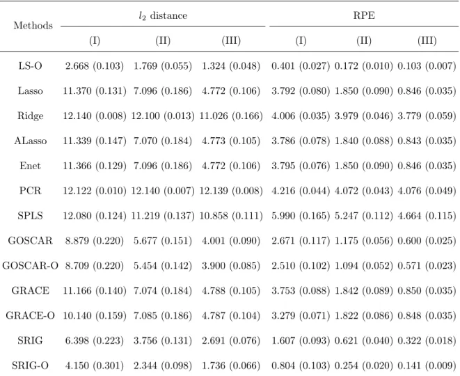
Table 2.5: Comparison of estimation and prediction (Example 3).
Methods
l2 distance RPE
(I) (II) (III) (I) (II) (III)
LS-O 2.668 (0.103) 1.769 (0.055) 1.324 (0.048) 0.401 (0.027) 0.172 (0.010) 0.103 (0.007)
Lasso 11.370 (0.131) 7.096 (0.186) 4.772 (0.106) 3.792 (0.080) 1.850 (0.090) 0.846 (0.035)
Ridge 12.140 (0.008) 12.100 (0.013) 11.026 (0.166) 4.006 (0.035) 3.979 (0.046) 3.779 (0.059)
ALasso 11.339 (0.147) 7.070 (0.184) 4.773 (0.105) 3.786 (0.078) 1.840 (0.088) 0.843 (0.035)
Enet 11.366 (0.129) 7.096 (0.186) 4.772 (0.106) 3.795 (0.076) 1.850 (0.090) 0.846 (0.035)
PCR 12.122 (0.010) 12.140 (0.007) 12.139 (0.008) 4.216 (0.044) 4.072 (0.043) 4.076 (0.049)
SPLS 12.080 (0.124) 11.219 (0.137) 10.858 (0.111) 5.990 (0.165) 5.247 (0.112) 4.664 (0.115)
GOSCAR 8.879 (0.220) 5.677 (0.151) 4.001 (0.090) 2.671 (0.117) 1.175 (0.056) 0.600 (0.025)
GOSCAR-O 8.709 (0.220) 5.454 (0.142) 3.900 (0.085) 2.510 (0.102) 1.094 (0.052) 0.571 (0.023)
GRACE 11.166 (0.140) 7.074 (0.184) 4.788 (0.105) 3.753 (0.088) 1.842 (0.089) 0.850 (0.035)
GRACE-O 10.140 (0.159) 7.085 (0.186) 4.787 (0.104) 3.279 (0.071) 1.822 (0.086) 0.848 (0.035)
SRIG 6.398 (0.223) 3.756 (0.131) 2.691 (0.076) 1.607 (0.093) 0.621 (0.040) 0.322 (0.018)
SRIG-O 4.150 (0.301) 2.344 (0.098) 1.736 (0.066) 0.804 (0.103) 0.254 (0.020) 0.141 (0.009)
acquires much lower FPR than the GOSCAR-O and GRACE-O methods. This indicates that GRACE and GOSCAR methods using the predictor graph edge-by-edge may lead to poor model selection results, although they can acquire competitive performance for es-timation and prediction. Compared with latent component approaches, SRIG has better performance than PCR while worse performance than SPLS. However, SRIG-O has better performance than PCR and SPLS in most cases.
Table 2.6: Comparison of model selection (Example 3).
Methods
FPR FNR
(I) (II) (III) (I) (II) (III)
LS-O 0.000 (0.000) 0.000 (0.000) 0.000 (0.000) 0.000 (0.000) 0.000 (0.000) 0.000 (0.000)
Lasso 0.152 (0.019) 0.467 (0.015) 0.481 (0.013) 0.793 (0.027) 0.129 (0.018) 0.011 (0.005)
Ridge 1.000 (0.000) 1.000 (0.000) 1.000 (0.000) 0.000 (0.000) 0.000 (0.000) 0.000 (0.000)
ALasso 0.155 (0.020) 0.469 (0.014) 0.473 (0.014) 0.776 (0.031) 0.124 (0.017) 0.011 (0.005)
Enet 0.233 (0.031) 0.467 (0.015) 0.481 (0.013) 0.716 (0.034) 0.129 (0.018) 0.011 (0.005)
PCR 1.000 (0.000) 1.000 (0.000) 1.000 (0.000) 0.000 (0.000) 0.000 (0.000) 0.000 (0.000)
SPLS 0.440 (0.050) 0.351 (0.044) 0.305 (0.042) 0.502 (0.053) 0.493 (0.046) 0.476 (0.049)
GOSCAR 0.292 (0.028) 0.378 (0.022) 0.380 (0.011) 0.438 (0.031) 0.060 (0.010) 0.004 (0.003)
GOSCAR-O 0.261 (0.024) 0.349 (0.016) 0.369 (0.012) 0.424 (0.030) 0.049 (0.009) 0.004 (0.003)
GRACE 0.220 (0.030) 0.472 (0.015) 0.481 (0.014) 0.711 (0.036) 0.120 (0.018) 0.011 (0.005)
GRACE-O 0.677 (0.058) 0.531 (0.028) 0.480 (0.014) 0.296 (0.055) 0.085 (0.015) 0.009 (0.004)
SRIG 0.216 (0.012) 0.266 (0.017) 0.245 (0.016) 0.109 (0.014) 0.015 (0.005) 0.000 (0.000)
SRIG-O 0.163 (0.018) 0.127 (0.018) 0.071 (0.015) 0.031 (0.018) 0.000 (0.000) 0.000 (0.000)
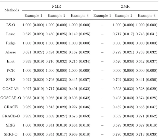
Table 2.7: Comparison of NMR and ZMR (Sample sizes: 40/40/400).
Methods
NMR ZMR
Example 1 Example 2 Example 3 Example 1 Example 2 Example 3
LS-O 1.000 (0.000) 1.000 (0.000) 1.000 (0.000) − 1.000 (0.000) 1.000 (0.000)
Lasso 0.679 (0.020) 0.480 (0.025) 0.149 (0.025) − 0.717 (0.017) 0.743 (0.031)
Ridge 1.000 (0.000) 1.000 (0.000) 1.000 (0.000) − 0.000 (0.000) 0.000 (0.000)
Alasso 0.681 (0.027) 0.494 (0.026) 0.167 (0.029) − 0.779 (0.021) 0.738 (0.032)
Enet 0.939 (0.019) 0.710 (0.032) 0.215 (0.034) − 0.520 (0.038) 0.642 (0.037)
PCR 1.000 (0.000) 1.000 (0.000) 1.000 (0.000) − 0.000 (0.000) 0.000 (0.000)
SPLS 0.922 (0.020) 0.703 (0.033) 0.445 (0.057) − 0.702 (0.038) 0.441 (0.056)
GOSCAR 0.927 (0.019) 0.717 (0.026) 0.491 (0.032) − 0.593 (0.032) 0.528 (0.029)
GOSCAR-O 0.933 (0.019) 0.966 (0.012) 0.505 (0.032) − 0.405 (0.040) 0.574 (0.028)
GRACE 0.989 (0.008) 0.813 (0.029) 0.227 (0.036) − 0.462 (0.048) 0.658 (0.037)
GRACE-O 0.989 (0.008) 0.809 (0.027) 0.676 (0.059) − 0.552 (0.040) 0.271 (0.052)
SRIG 1.000 (0.000) 0.841 (0.019) 0.864 (0.018) − 0.579 (0.020) 0.627 (0.018)
SRIG-O 1.000 (0.000) 0.844 (0.017) 0.969 (0.018) − 0.780 (0.020) 0.713 (0.030)
[−indicates that value is not available since there are no edges between useless predictors.]
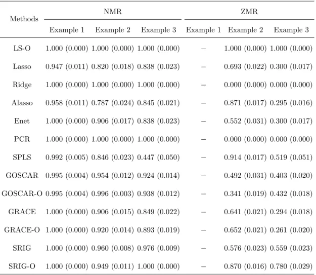
Table 2.8: Comparison of NMR and ZMR (Sample sizes: 80/80/400).
Methods
NMR ZMR
Example 1 Example 2 Example 3 Example 1 Example 2 Example 3
LS-O 1.000 (0.000) 1.000 (0.000) 1.000 (0.000) − 1.000 (0.000) 1.000 (0.000)
Lasso 0.947 (0.011) 0.820 (0.018) 0.838 (0.023) − 0.693 (0.022) 0.300 (0.017)
Ridge 1.000 (0.000) 1.000 (0.000) 1.000 (0.000) − 0.000 (0.000) 0.000 (0.000)
Alasso 0.958 (0.011) 0.787 (0.024) 0.845 (0.021) − 0.871 (0.017) 0.295 (0.016)
Enet 1.000 (0.000) 0.906 (0.017) 0.838 (0.023) − 0.552 (0.031) 0.300 (0.017)
PCR 1.000 (0.000) 1.000 (0.000) 1.000 (0.000) − 0.000 (0.000) 0.000 (0.000)
SPLS 0.992 (0.005) 0.846 (0.023) 0.447 (0.050) − 0.914 (0.017) 0.519 (0.051)
GOSCAR 0.995 (0.004) 0.954 (0.012) 0.924 (0.014) − 0.492 (0.031) 0.403 (0.020)
GOSCAR-O 0.995 (0.004) 0.996 (0.003) 0.938 (0.012) − 0.341 (0.019) 0.432 (0.018)
GRACE 1.000 (0.000) 0.906 (0.015) 0.849 (0.022) − 0.641 (0.021) 0.294 (0.018)
GRACE-O 1.000 (0.000) 0.920 (0.014) 0.893 (0.019) − 0.652 (0.021) 0.261 (0.020)
SRIG 1.000 (0.000) 0.960 (0.008) 0.976 (0.009) − 0.576 (0.023) 0.559 (0.023)
SRIG-O 1.000 (0.000) 0.949 (0.011) 1.000 (0.000) − 0.870 (0.016) 0.780 (0.029)
[−indicates that value is not available since there are no edges between useless predictors.]
In conclusion, the simulation results indicate that our proposed SRIG method can make use of the structure information among predictors efficiently and performs well for both estimation, prediction and model selection.
2.5.2 Sensitivity Study
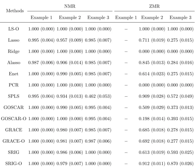
Table 2.9: Comparison of NMR and ZMR (Sample sizes: 120/120/400).
Methods
NMR ZMR
Example 1 Example 2 Example 3 Example 1 Example 2 Example 3
LS-O 1.000 (0.000) 1.000 (0.000) 1.000 (0.000) − 1.000 (0.000) 1.000 (0.000)
Lasso 0.995 (0.004) 0.957 (0.009) 0.985 (0.007) − 0.711 (0.019) 0.275 (0.015)
Ridge 1.000 (0.000) 1.000 (0.000) 1.000 (0.000) − 0.000 (0.000) 0.000 (0.000)
Alasso 0.987 (0.006) 0.906 (0.014) 0.985 (0.007) − 0.845 (0.013) 0.284 (0.016)
Enet 1.000 (0.000) 0.990 (0.005) 0.985 (0.007) − 0.614 (0.023) 0.275 (0.015)
PCR 1.000 (0.000) 1.000 (0.000) 1.000 (0.000) − 0.000 (0.000) 0.000 (0.000)
SPLS 0.995 (0.004) 0.934 (0.013) 0.462 (0.053) − 0.909 (0.028) 0.572 (0.049)
GOSCAR 1.000 (0.000) 0.990 (0.005) 0.995 (0.004) − 0.509 (0.029) 0.373 (0.013)
GOSCAR-O 1.000 (0.000) 1.000 (0.000) 0.995 (0.004) − 0.198 (0.014) 0.393 (0.015)
GRACE 1.000 (0.000) 0.980 (0.007) 0.985 (0.007) − 0.685 (0.018) 0.278 (0.015)
GRACE-O 1.000 (0.000) 0.981 (0.007) 0.987 (0.006) − 0.692 (0.018) 0.277 (0.015)
SRIG 1.000 (0.000) 0.986 (0.006) 1.000 (0.000) − 0.613 (0.019) 0.593 (0.025)
SRIG-O 1.000 (0.000) 0.979 (0.007) 1.000 (0.000) − 0.912 (0.011) 0.870 (0.026)
[−indicates that value is not available since there are no edges between useless predictors.]
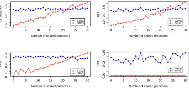
To this end, we evaluate the performance of SRIG on a series of data sets with changing predictor graphs. Fix p = 100, σ = 3, s0 = 20, and β0 = (20,2,2,· · ·,2,0,0,· · · ,0). For each p∗ = 0,1, . . . ,30, we generate the predictor matrix X from N(0,Ω−1), where
Ω = L+ 2|λmax(L)|Ip. Here, Lii = 2 for each 1 ≤ i ≤ p, L1i = Li1 = 0.3 for each 1≤i≤(s0+p∗),L(s0+1)i =Li(s0+1)= 0.3 for each (s0+ 1)≤i≤p, andLij = 0 otherwise.
Finally, Ωis standardized to have unit diagonals.
For this study, the true precision matrix Ωis used to construct the predictor graphG. The neighborhoods of the useful predictor X1 and the useless predictor Xs0+1 are N1 =
{1,2, . . . , s0+p∗}andNs0+1 ={s0+1, s0+2, . . . , p}, respectively. The number of predictors
0 5 10 15 20 25 30
2.5
4.0
5.5
Number of shared predictors
L2_distance Lasso
SRIG
0 5 10 15 20 25 30
1.0
2.0
3.0
Number of shared predictors
RPE
Lasso SRIG
0 5 10 15 20 25 30
0.05
0.20
0.35
Number of shared predictors
FPR
Lasso SRIG
0 5 10 15 20 25 30
0.00
0.03
0.06
Number of shared predictors
FNR
Lasso SRIG
Figure 2.2: Sensitivity study of the SRIG method.
condition (A2) is satisfied when p∗ = 0 and will be violated more and more seriously as p∗
increases. Based on this example, we study the robustness of SRIG asp∗ changes gradually from 0 to 30. For each p∗, we also evaluate the performance of Lasso method. The sample sizes are fixed as 80/80/400.
Figure 2.2 shows the performances of SRIG and Lasso method as the number of shared predictors p∗ increases. It indicates that Lasso method is more robust than our proposed SRIG method to the intersection between the neighborhood of useful predictors and the neighborhood of useless predictors. One possible reason is that Lasso does not use the predictor graph information directly. For our proposed SRIG method, as p∗ increases, the condition (A2) is more and more violated and the performance of SRIG gets worse. As shown in Figure 2.2, if the condition (A2) is not violated seriously, our proposed SRIG method still has better performance than the Lasso method. However, if (A2) is violated seriously (i.e.,p∗>25), Lasso method performs better than our proposed SRIG method.
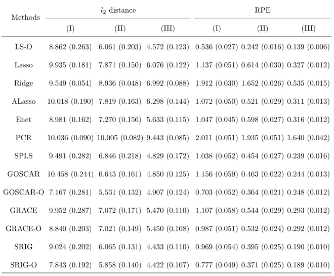
Table 2.10: Comparison of estimation and prediction (Adjusted Example 2).
Methods
l2 distance RPE
(I) (II) (III) (I) (II) (III)
LS-O 8.862 (0.263) 6.061 (0.203) 4.572 (0.123) 0.536 (0.027) 0.242 (0.016) 0.139 (0.006)
Lasso 9.935 (0.181) 7.871 (0.150) 6.076 (0.122) 1.137 (0.051) 0.614 (0.030) 0.327 (0.012)
Ridge 9.549 (0.054) 8.936 (0.048) 6.992 (0.088) 1.912 (0.030) 1.652 (0.026) 0.535 (0.015)
ALasso 10.018 (0.190) 7.819 (0.163) 6.298 (0.144) 1.072 (0.050) 0.521 (0.029) 0.311 (0.013)
Enet 8.981 (0.162) 7.270 (0.156) 5.633 (0.115) 1.047 (0.045) 0.598 (0.027) 0.316 (0.012)
PCR 10.036 (0.090) 10.005 (0.082) 9.443 (0.085) 2.011 (0.051) 1.935 (0.051) 1.640 (0.042)
SPLS 9.491 (0.282) 6.846 (0.218) 4.829 (0.172) 1.038 (0.052) 0.454 (0.027) 0.239 (0.016)
GOSCAR 10.458 (0.244) 6.643 (0.161) 4.850 (0.125) 1.156 (0.059) 0.463 (0.022) 0.244 (0.013)
GOSCAR-O 7.167 (0.281) 5.531 (0.132) 4.907 (0.124) 0.703 (0.052) 0.364 (0.021) 0.248 (0.012)
GRACE 9.952 (0.287) 7.072 (0.171) 5.470 (0.110) 1.107 (0.058) 0.544 (0.029) 0.293 (0.012)
GRACE-O 8.840 (0.203) 7.021 (0.149) 5.450 (0.108) 0.987 (0.051) 0.532 (0.024) 0.292 (0.012)
SRIG 9.024 (0.202) 6.065 (0.131) 4.433 (0.110) 0.969 (0.054) 0.395 (0.025) 0.190 (0.010)
SRIG-O 7.843 (0.192) 5.858 (0.140) 4.422 (0.107) 0.777 (0.049) 0.371 (0.025) 0.189 (0.010)
Adjusted Example 2: This example is almost the same as Example 2. We only change the true coefficient vector in Example 2 to
β0 = (3,· · · ,3
| {z } 5
,0,· · ·,0
| {z } 5
,3,· · ·,3
| {z } 5
,0,· · · ,0
| {z } 5
,3,· · · ,3
| {z } 5
,0,· · ·,0
| {z } 75
).
Table 2.11: Comparison of model selection (Adjusted Example 2).
Methods
FPR FNR
(I) (II) (III) (I) (II) (III)
LS-O 0.000 (0.000) 0.000 (0.000) 0.000 (0.000) 0.000 (0.000) 0.000 (0.000) 0.000 (0.000)
Lasso 0.144 (0.009) 0.188 (0.014) 0.184 (0.011) 0.340 (0.017) 0.128 (0.015) 0.029 (0.006)
Ridge 1.000 (0.000) 1.000 (0.000) 1.000 (0.000) 0.000 (0.000) 0.000 (0.000) 0.000 (0.000)
ALasso 0.109 (0.010) 0.114 (0.013) 0.122 (0.010) 0.352 (0.019) 0.144 (0.015) 0.051 (0.008)
Enet 0.362 (0.032) 0.343 (0.028) 0.229 (0.012) 0.151 (0.016) 0.045 (0.008) 0.019 (0.005)
PCR 1.000 (0.000) 1.000 (0.000) 1.000 (0.000) 0.000 (0.000) 0.000 (0.000) 0.000 (0.000)
SPLS 0.198 (0.034) 0.082 (0.015) 0.076 (0.016) 0.277 (0.026) 0.155 (0.019) 0.049 (0.009)
GOSCAR 0.246 (0.018) 0.496 (0.019) 0.651 (0.019) 0.252 (0.018) 0.013 (0.004) 0.001 (0.001)
GOSCAR-O 0.460 (0.036) 0.575 (0.022) 0.739 (0.018) 0.047 (0.011) 0.003 (0.002) 0.001 (0.001)
GRACE 0.242 (0.030) 0.233 (0.020) 0.193 (0.010) 0.248 (0.021) 0.060 (0.009) 0.011 (0.003)
GRACE-O 0.316 (0.039) 0.234 (0.020) 0.193 (0.011) 0.144 (0.016) 0.064 (0.010) 0.011 (0.003)
SRIG 0.131 (0.010) 0.183 (0.014) 0.132 (0.011) 0.293 (0.019) 0.053 (0.010) 0.007 (0.003)
SRIG-O 0.179 (0.013) 0.164 (0.013) 0.119 (0.010) 0.143 (0.014) 0.039 (0.009) 0.008 (0.004)
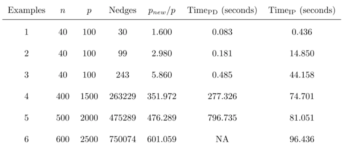
2.5.3 PD method v.s. IP algorithm
In this subsection, we compare the computational costs of the PD method and our proposed IP algorithm by some examples. Besides the Examples 1-3 shown in Section 2.5.1, we also consider the following three high dimensional examples:
Example 4: n = 400, p = 1500, s0 = 25, σ = 5, and the true coefficient vector β0 = (1,1,· · · ,1,0,· · ·,0). The predictors are generated as follows.
Xj =Z1+xj, Z1 ∼N(0,1), 1≤j≤25,
Table 2.12: Time comparison between PD method and IP algorithm.
Examples n p Nedges pnew/p TimePD (seconds) TimeIP (seconds)
1 40 100 30 1.600 0.083 0.436
2 40 100 99 2.980 0.181 14.850
3 40 100 243 5.860 0.485 44.158
4 400 1500 263229 351.972 277.326 74.701
5 500 2000 475289 476.289 796.735 81.051
6 600 2500 750074 601.059 NA 96.436
[Nedges: the number of edges in the graphG;pnew: the number of predictors in the duplicated
predictor matrix; TimePD: computing time of the PD method; TimeIP: computing time of the IP
algorithm; NA: out of memory.]
wherexj i.i.d∼ N(0,1), j = 1,2, . . . ,50 andΩ∗ =L+δI. Each off-diagonal entry inLis generated independently and equals to 0.5 with probability 0.25, or 0 with probability 0.75. The diagonal entry ofLis 0. Here,δ is chosen such that the conditional number of Ω∗ is equal top−50. Finally,Ω∗ is standardized to have unit diagonals.
Example 5: n= 500, p= 2000 and the other setup is the same as Example 4.
Example 6: n= 600, p= 2500 and the other setup is the same as Example 4.
PD method. For Example 6, the PD method using gglasso package breaks down due to out of memory while our proposed IP algorithm still works well. In this case, the proposed IP algorithm is very desirable.
2.6 Real Data Example
Alzheimer’s disease (AD) is one of the most common forms of dementia characterized by progressive cognitive and memory deficits. The increasing incidence of AD makes the disease a very important health issue and a huge financial burden for both patients and governments ((Hebert et al., 2001)). In the practical diagnosis of AD, the Mini Mental State Examination (MMSE) ((Folstein et al., 1975)) score is a very important reference. MMSE is a brief 30-point questionnaire test that is used to screen for cognitive impairment. It can be used to examine patient’s arithmetic, memory and orientation. Generally, any score greater than or equal to 27 points (out of 30) indicates a normal cognition. Below this, MMSE score can indicate severe (≤9 points), moderate (10-18 points) or mild (19-24 points) cognitive impairment ((Mungas, 1991)). As more and more treatments are being developed and evaluated, it is very important to develop diagnostic and prognostic biomarkers that can predict which individuals are relatively more likely to progress clinically. At present, structural magnetic resonance imaging (MRI) is one of the most popular and powerful techniques for the diagnosis of AD. It is very interesting to use MRI data to predict MMSE score which can be used to diagnose the current disease status of AD.
Figure 2.3: Estimated graph of 93 MRI features.
103 subjects. For each subject, there are one MMSE score and 93 MRI features. We treat MMSE score as the response variable and MRI features as predictors in our model.
Lasso Ridge Alasso Enet GOSCAR GRACE PCR SPLS SRIG
0.55
0.60
0.65
0.70
Mean Squared Error
Figure 2.4: Comparison of MSE for various methods on the ADNI data set.