SKEWNESS AND DISPERSION OF OPINION AND THE CROSS SECTION OF STOCK RETURNS
Jinghan Meng
A dissertation submitted to the faculty of the University of North Carolina at Chapel Hill in partial fulfillment of the requirements for the degree of Doctor of Philosophy in the Department of Finance in the Kenan-Flagler Business School.
Chapel Hill 2014
Approved by:
Riccardo Colacito Eric Ghysels
ABSTRACT
Jinghan Meng: Skewness and Dispersion of Opinion and the Cross Section of Stock Returns. (Under the direction of Riccardo Colacito.)
ACKNOWLEDGMENTS
When I am writing this dissertation, I feel so grateful to all the wonderful people I have met during such a long and challenging PhD journey at the Kenan-Flagler Business School. This dissertation would not have existed without their generous care, patience, support and e↵orts.
I cannot express my gratitude enough to my advisors Riccardo Colacito and Eric Ghysels for their never stopping mentor, support, encouragement and understanding during the past four years. I have learned so many invaluable things from them, not only about how to do research, but more importantly, about how to be a qualified scholar and a responsible professor. All I have learned from them give me the determination and confidence to start my academic career after graduation. A special thanks also goes to Christian Lundblad. He provided generous comments on my job market paper and extensive advice on the job interviews and presentations. I will never forget his strong support during the job-market.
I need to thank my dissertation committe members Chotibhak Jotikasthira and Anh Le for their comments and suggestions.
I also feel very lucky to meet a wonderful community of PhD students in finance department. They provided me with intellectual input, challenge and advice. I have received a lot of feedbacks and suggestions during the PhD seminars and the discussions with them. I am also thankful to my dear friends outside finance program, including but not limited to Yihe Zhao, Songcui Hu, Yan Liu, Qi Wang and Han Xia.
TABLE OF CONTENTS
LIST OF TABLES . . . vii
LIST OF FIGURES . . . viii
Introduction . . . 1
1.1 The Model . . . 3
1.1.1 Propositions . . . 5
1.1.2 Testable Hypotheses . . . 7
1.2 Measuring Heterogeneity of Beliefs . . . 9
1.2.1 Measures of Heterogeneity . . . 9
1.2.2 Summary Statistics . . . 11
1.3 Using Dispersion and Skewness in Beliefs to Forecast Returns . . . 12
1.3.1 Portfolio Sorts Based on Dispersion . . . 12
1.3.2 Double Sorts Based on Dispersion and Skewness . . . 13
1.3.3 Firm Characteristics of Dispersion-Skewness Portfolios . . . 14
1.3.4 Triple Sorts . . . 16
1.3.5 Four-Factor Model Time-Series Tests . . . 17
1.4 Robustness Checks . . . 19
1.4.1 Subperiod Analysis . . . 19
1.4.2 Di↵erent Analyst Coverage Cuto↵ . . . 19
1.4.3 Portfolio Updating Frequency and Holding Period . . . 20
1.5.1 Comparison with Stock Recommendations . . . 21
1.5.2 Comparison with Ex Ante Variance and Skewness . . . 22
1.6 Concluding Remarks . . . 22
APPENDIX . . . 45
LIST OF TABLES
1.1 Summary Statistics . . . 24
1.2 Returns of Portfolios Formed on Size and Dispersion . . . 25
1.3 Returns to Dispersion Strategies with Di↵erent Analyst Coverage . . . 26
1.4 Returns of Portfolios Formed on Dispersion and Skewness . . . 27
1.5 Characteristics of The Dispersion-Skewness Portfolios . . . 28
1.6 Characteristics of The Dispersion-Skewness Portfolios (Cont0d) . . . 29
1.7 Returns of Portfolios Formed on Average, Dispersion and Skewness . . . 30
1.8 Returns of Triple-Sorted Portfolios: Size, Book-To-Market . . . 31
1.9 Returns of Triple-Sorted Portfolios: Momentum, Illiquidity . . . 32
1.10 Four-Factor Model Time-Series Tests . . . 33
1.11 Subperiod and Di↵erent Analyst Coverage . . . 34
1.12 Di↵erent Holding Period and Updating Frequency . . . 35
1.13 I/B/E/S Earnings Forecasts and Stock Recommendations . . . 36
1.14 Ex Ante Variance And Skewness . . . 37
LIST OF FIGURES
1.1 Skew-Normal Distribution with Di↵erent and ⌫ . . . 4
1.2 Equilibrium Prices . . . 8
1.3 Owen’s T Function with Di↵erent Skewness Parameter⌫. . . 39
Introduction
Empirical researchers have not yet reached an agreement on the role of analysts’ di↵erence of opinions on future stocks’ returns. Diether, Malloy, and Scherbina (2002) and Chen, Hong, and Stein (2002) find a negative relation between dispersion and stock returns, while Anderson, Ghysels, and Juergens (2005) document the opposite result.
In this dissertation, we document that double sorting on the degree of asymmetry (skewness) of analysts’ forecasts and on the extent of dispersion o↵ers the possibility of reconciling the existing views in the literature. We use analysts’ short-term earnings forecasts as proxies for agents’ beliefs, and measure the asymmetry of beliefs as the skewness of the distribution of these forecasts for each individual stock. We document several novel empirical findings.
First, the relationship between dispersion of beliefs and subsequent returns is opposite for the stocks with positive skewness in beliefs and otherwise similar stocks with negative skewness. Specifically, when skewness is negative, future returns are decreasing in the degree of dispersion of analysts’ earnings forecasts. A dispersion strategy (buying the portfolio of stocks in the lowest dispersion quintile and shorting the portfolio of stocks in highest dispersion quintile) for the most-negative-skewness quintile generates a 0.65% monthly return on average. When skewness is positive, future returns are increasing in the degree of dispersion, but the return di↵erential is moderate. These findings provide a potential explanation for the contradicting dispersion e↵ect documented in the literature.
We also provide a theoretical explanation for our findings. Many theoretical models have studied the relationship between dispersion of beliefs and subsequent returns. Miller (1977), Jarrow (1980), Mayshar (1983), Diamond and Verrecchia (1987), and Chen, Hong, and Stein (2002) argue that in the presence of short-sales constraints, stock prices only reflect the valuation of optimistic investors and are higher than the true value. Therefore, higher dispersion of opinions should predict lower stock returns. Harrison and Kreps (1978), and Morris (1996) link heterogeneous beliefs to investor speculative behavior and show that with short-sales constraints, smaller di↵erences in opinion generate larger speculative premium. On the other hand, Williams (1977), Abel (1989), Detemple and Murthy (1994), Basak (2000), and Anderson, Ghysels, and Juergens (2005) view heterogeneity of beliefs as a fundamental risk of the stock and argue that higher dispersion of beliefs should predict higher stock returns.
We develop a static model that incorporates both the degree of dispersion and asymmetry of agents’ beliefs about stock fundamentals. We show that it can account for these stylized empirical facts described above. In our model, a continuum of risk-neutral agents have identical preference and endowment, but di↵erent beliefs about conditional expectation of stock dividend stream. We explicitly model the agents’ beliefs about conditional mean as following a skew-normal distribution (Azzalini 1985 ). The skew-normal distribution provides a convenient way of characterizing asym-metry in opinions. Agents make decisions based on the their perceived profitability of buying or selling a stock after paying transaction costs. In equilibrium, prices clear the markets and reflect the heterogenous beliefs of all agents who actually trade the stock.
Our model implies that the relationship betwen dispersion of beliefs and returns essentially depends on the sign of the skewness. When transaction costs associated with buying and selling a stock are similar, the stock is underpriced when skewness is positive and higher dispersion of beliefs predicts higher stock returns; Conversely, when skewness is negative, the stock is overpriced and higher dispersion of beliefs predicts lower returns. When skewness is zero, the dispersion of beliefs has no e↵ect on stock returns. Note that our model does not impose the assumption of short-sales constraints, which makes the last argument consistent with the findings in Miller’s (1997) model (also see, e.g., Chen, Hong, and Stein (2002), etc.). Miller’s (1977) model with short-sales constraints can be viewed as a special case of our model with asymmetric transaction costs.
model and proposes three testable hypothese. Section 3 discusses the data and our empirical measures of heterogeneity. Section 4 examines the relation between dispersion and skewness of analysts’ earnings forecasts and subsequent returns. Section 5 and 6 provides various robustness analysis and some additional discussions. Section 7 concludes.
1.1
The Model
In this section, we present a static model that incorporates both the degree of dispersion and asymmetry in agents’ beliefs about conditional expectation of future dividend, and demonstrate how heterogenous beliefs a↵ect stock prices through their trading decisions. In this dissertation, we solely focus on the heterogeneity of beliefs among agents, and exclude the other possible sources of heterogeneity, such as preferences and endowments. For simplicity, we also disregard risk-sharing among di↵erent asset classes.
The model has one period with two dates 0, 1. There is a single stock which will be liquidated at date 1. A continuum of agents, indexed byi, are risk-neutral and can borrow or lend at a risk-free interest rate of zero. With no loss of generality, we assume that agents have one unit of endowment at time t= 0 (an agent with N units of endowments is equivalent to N agents who have one unit of endowment and hold identical belief). They can buy or sell at most one share of the stock. The liquidation value of the stock is V1 = ¯V1+"1, where ¯V1 is the true conditional expectation of stock
price at timet= 1. Agents disagree about conditional mean ¯V1, but agree on the higher moments
of V1.1 At time 0, agent i has a stock valuation Vi = Ei,0(V1) and observes the market price P.
Transaction cost of buying or shorting the stock isc 0 (later we will relax this assumption and allow for asymmetry in the costs). Agents make trading decisions based on their perceived profit: buy if Vi > P +c, sell if Vi < P c, and take no action if P c < Vi < P +c. Since they are risk-neutral, the amount of trade is 1 or 0 share of the stock.
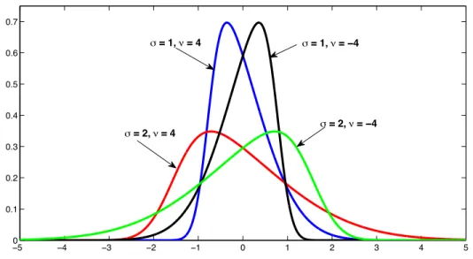
We assume that agents’ conditional expecation of the stock valuation Vi follows a skew-normal distribution SKN(µ, ,⌫) as defined by Azzalini (1985). Parameters µ, and ⌫ govern average,
1Anderson, Ghysels, and Juergens (2005) have a formal discussion about this assumption. Specifically, we do not have
information about individual agent’s perceived distribution ofV1. Therefore, we assume that it is entirely specified
−5 −4 −3 −2 −1 0 1 2 3 4 5 0
0.1 0.2 0.3 0.4 0.5 0.6 0.7
σ = 1, ν = −4
σ = 2, ν = −4
σ = 2, ν = 4
σ = 1, ν = 4
Figure 1.1: Skew-Normal Distribution with Di↵erent and ⌫
The parameter governs the volatility, ⌫ governs the skewness of the distribution.
dispersion and asymmetry of the distribution, respectively.2 The skew-normal distribution provides
a convenient way of characterizing departures from normality which may consist in negatively or positively skewed beliefs (see Figure 1.1). The computational attractiveness of this distribution is that the first four centered moments are available in closed form.3 Moreover, the skewness of a skew-normal distribution always sits between -1 and 1. This property enables us to focus on a general case that agents’ beliefs are clustered about the mean with reasonable degree of time-varying asymmetry, rather than exceptional cases in which there are a number of extremely pessimistic or optimistic agents and the degree of asymmetry is dramatic.4 In Appendix A1, we introduce the properties of skew-normal distribution that will be used in later discussions.
To exclude the e↵ect of average opinion, we assume that the skew-normal distributionSKN(µ, ,⌫) has a fixed mean of ¯V1, then µ = ¯V1
q 2
⇡. Thus on average the agents have the right
valua-tion, but there is heterogeneity among them, with the degree of dispersion parameterized by and asymmetry parameterized by⌫. Note that agents’ average beliefs does not necessarily equal to the true conditional mean, but since our primary interest is thedi↵erenceof their valuations, including
2See also Colacito, Ghysels, and Meng (2013) who use the skew-normal distribution in expected macro fundamentals.
3Specifically: mean =µ+ q2
⇡, variance =
2⇣1 22
⇡ ⌘
, skewness = 4 ⇡
2
( p2/⇡)3
(1 2 2/⇡)3/2, where = p⌫
1+⌫2.
4Some other widely used distribution functions, e.g., log-normal distribution, chi-squared distribution, and gamma
a bias in the average beliefs does not change our results about the e↵ect of heterogeneous beliefs. We denote the pdf of the skew-normal distribution asf(x; ,⌫), and denote cdf asF(x; ,⌫). Then the aggregate demand of the stock is
QD(P; ,⌫) =
Z 1
P+c
f(Vi; ,⌫)dVi= 1 F(P+c; ,⌫) (1.1)
and the aggregate supply of the stock is
QS(P; ,⌫) =
Z P c
1
f(Vi; ,⌫)dVi =F(P c; ,⌫) (1.2)
The market clearing condition is Fe(P; ,⌫) = QD(P; ,⌫) QS(P; ,⌫) = 0. The equilibrium price, denoted by P⇤( ,⌫), clears the market.5 Assuming that agents’ heterogeneous beliefs have an impact on current stock price, but not its liquidation value, then the expected future return is
¯
V1 P⇤( ,⌫).
Next, we discuss the properties of the equilibrium price as a function of dispersion and skewness of agents’ beliefs and the transaction costc. Proofs of all the following propostions are in Appendix A2.
1.1.1 Propositions
Proposition 1. For any transaction cost c 0, there exists a unique equilibrium price P⇤( ,⌫)
that clears the market, i.e., the function
e
F(P; ,⌫) =QD(P; ,⌫) QS(P; ,⌫) (1.3)
has a unique solution P⇤( ,⌫).
In general, P⇤( ,⌫) does not have a closed-form expression due to the complication of skew-normal distribution function. Fortunately, however, we still manage to show the circumstances when equilibrium priceP⇤( ,⌫) deviate from the true value ¯V1, and how the deviation change with
5One may argue that in reality, agents’ valuation cannot be arbitrarily extreme, therefore the distribution of agents’
the degree of dispersion of opinion , the asymmetry of opinion ⌫, as well as the transaction cost c. They are discussed in Proposion 2 and 3.
Proposition 2. Fix the transaction cost c >0.
(i) For any given ⌫ > 0, there exists a unique positive ⇤(⌫, c) such that when > ⇤(⌫, c), the equilibrium price P⇤( ,⌫)<V¯1;
(ii) For any given ⌫ < 0, there exists a unique positive ⇤(⌫, c) such that when > ⇤(⌫, c), the equilibrium price P⇤( ,⌫)>V¯1.
(iii) When ⌫= 0, the equilibrium price P⇤( ,⌫) = ¯V1; (iv) For any given ⌫ and costsc1, c2 >0, we have
⇤(⌫,c1)
c1 =
⇤(⌫,c2)
c2 . Whenc= 0,
⇤(⌫, c) = 0.
Prior studies (e.g., Miller (1977), Jarrow (1980), and Chen, Hong, and Stein (2002) argue that without short-sales constraints, di↵erences of opinion have no e↵ect on prices. Proposition 2 tells us that this is the case only when there is no asymmetry in the beliefs. When the agents’ beliefs are skewed, heterogeneity of agents’ beliefs will a↵ect the level of stock prices, and hence has ability to forecast subsequent returns. Moreover, the relation between dispersion of beliefs and subsequent returns are opposite for the stocks with positive skewness in beliefs and otherwise similar stocks with negative skewness in beliefs, as long as the magnitude of the dispersion exceeds a minimum threshold ⇤(⌫, c). Intuitively, in an extreme case of no dispersion in opinion but high transaction cost, there is no profit from buying or shorting the stock. All agents will then sit on the fence. Hence, a minimum amount of dispersion is necessary in our model to allow the agents with optimistic or pessimistic opinion to have positive perceived profit from the trades. Again, ⇤(⌫, c) typically does not have a closed-form expression. Proposition 2 shows that ⇤(⌫, c) is proportional to transaction cost c. Figure 1.4 in Appendix A2 plots ⇤(⌫, c) as a function of asymmetry parameter ⌫ when transaction costc. The range of ⇤(⌫, c) is between 0 and 1.72.
Proposition 3. Fix the transaction cost c 0.
Proposition 3 shows that when skewness is positive, greater divergence in opinion leads to a lower stock price and therefore a higher subsequent return. On the contrary, when skewness is negative, greater divergence in opinion leads to a lower subsequent return.
Last, we briefly discuss the relation between our model and Miller’s model with short-sales constraints. We relax the assumption of symmetric costs associated with buying and selling a stock. Instead, we assume that the cost of short-selling a stock (denoted by c ) is much higher than the cost of buying a stock (denoted by c+). Then the di↵erence between total demand and
supply of the stock defined in equation 1.6 is
e
F(P; ,⌫) =QD(P; ,⌫) QS(P; ,⌫) = 1 F(P +c+; ,⌫) F(P c ; ,⌫). (1.4)
When c c+, F(P c ; ,⌫) is close to 0 no matter of the sign of ⌫. To solve F(Pe ; ,⌫) ⇡
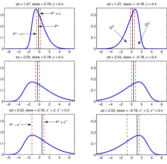
1 F(P +c+; ,⌫) = 0, we need a very positive equilibrium price P⇤ 0 to clear the market. In other words, with short-sales constraints, the stock is always overpriced. Even if the cost of short selling a stock is less extreme, this asymmetry in the costs will enhance the dispersion e↵ect when skewness is negative, and weaken the dispersion e↵ect when skewness is positive. Figure 1.2 visually illustrates the equilibrium price P⇤ in di↵erent skew-normal distributions, as well as in the case with short-sales constraints. All these distributions are centered at zero. Top four panels illustrate the models when transaction cost is symmetric. When skewness is positive (left panels), the equilibrium prices P⇤ depicted in solid line are less than zero and decrease with dispersion. When skewness is positive (right panels), the equilibrium prices P⇤ are positive and increase with dispersion. Two plots in the bottom panels demonstrate the models with high short-sales costs. P⇤ is positive no matter of the sign of skewness. Table 1.15 in Appendix A2 reports numerical solutions ofP⇤( ,⌫) with a variety choices of dispersion parameter , asymmetry parameter⌫ and transaction cost c. The mean of these skew-normal distributions ¯V1 are set to be zero, so the sign
of P⇤( ,⌫) indicates whether the stock is under or overpriced.
1.1.2 Testable Hypotheses
In the following empirical analysis, we test three hypotheses that are implied by Proposition 1 - 3.
−6 −4 −2 0 2 4 6 0
0.1 0.2 0.3
sd = 1.27, skew = 0.78, c = 0.4
−6 −4 −2 0 2 4 6
0 0.1 0.2 0.3
sd = 1.27, skew = −0.78, c = 0.4
−6 −4 −2 0 2 4 6
0 0.1 0.2 0.3
sd = 2.53, skew = 0.78, c = 0.4
−6 −4 −2 0 2 4 6
0 0.1 0.2 0.3
sd = 2.53, skew = −0.78, c = 0.4
−6 −4 −2 0 2 4 6
0 0.1 0.2 0.3
sd = 2.53, skew = 0.78, c− = 2, c+ = 0.4
−6 −4 −2 0 2 4 6
0 0.1 0.2 0.3
sd = 2.53, skew = −0.78, c− = 2, c+ = 0.4 P*
P* + c
P* − c− P* − c
P* + c+
QS Q
D
Figure 1.2: Equilibrium Prices
skewed, future returns are decreasing in the degree of dispersion of agents’ beliefs.
Hypothesis 2. When the distribution of agents’ beliefs about the stock fundamentals is positively
skewed, future returns are increasing in the degree of dispersion of agents’ beliefs. This dispersion
e↵ect will be weakened when short selling the stock is more costly than buying the stock.
Hypothesis 3. When the dispersion of agents’ beliefs is relatively large, a positive skewness in
1.2
Measuring Heterogeneity of Beliefs
Our data on analysts’ earnings forecasts come from the Institutional Brokers Estimate System (I/B/E/S). Monthly stock returns, prices, and trading volume are drawn from the Center for Research in Securities Prices (CRSP) monthly tape. Data used to compute book value of the stock are obtained from COMPUSTAT. We follow literature convention and limit the sample to U.S. common stocks listed on the NYSE, AMEX and Nasdaq. Stocks with monthly share prices less than $5 are excluded. Our sample period runs from January 1983 through December 2012.
The standard I/B/E/S data adjusted historically for stock splits are subject to reporting inac-curacy arised from the rounding issue, as discussed in details by Diether, Malloy, and Scherbina (2002). So we conduct the analysis using the raw forecast data from I/B/E/S Unadjusted De-tail History file. Stocks historical split adjustment factor are obtained from CRSP. Each month, it tracks all the individual analysts’ forecasts of earnings per share (EPS) for current fiscal year (FY1), two fiscal years ahead (FY2), and up to ten fiscal years ahead (FY10), starting in January 1983.
1.2.1 Measures of Heterogeneity
It has been widely discussed that the disagreement among analysts about expected earnings is a good proxy for investors’ heterogeneous beliefs. However, there is no consensus on the choice of forecast period. Diether, Malloy, and Scherbina (2002) use the short-term forecasts (FY1) forecasts, while Anderson, Ghysels, and Juergens (2005) consider both short-term and long-term forecasts (FY5). During our sample period, I/B/E/S contains the FY1 earnings estimates of 19,524 analysts covering 12,787 firms, and FY5 earnings estimates of 3,004 analysts covering 4,867 firms. Concerned with the accuracy of dispersion and skewness estimates, we need a reasonably large cross-analyst size for each individual stocks. On average, about 17% of the firms with FY1 earnings forecasts and only 2% of the firms with FY5 earnings forecasts are covered by eight or more analysts. So in this dissertation, we measure agents’ beliefs using analysts’ FY1 earnings forecasts and limit our sample to the stocks that are covered by eight or more analysts.6
6We repeat all the analysis using di↵erent analyst coverage cuto↵s, from at least 5 analysts to at least 10 analysts.
In each month, we compute the cross-analyst average, standard deviation and skewness of the analysts’ FY1 earnings forecasts for each individual stock. The dispersion of analysts’ earnings forecasts is defined as the standard deviation of FY1 earnings forecasts scaled by the absolute value of the average of forecasts. We define the analyst coverage of a stock in any given month as the number of analysts who report at least one FY1 earnings estimate during that month. Higher moments are sensitive to the extreme observations and we detect that some stocks have apparent outliers which appear to be errors when analysts report their estimates. So in each month, we remove observations in the top 0.5% and bottom 0.5% of the cross-sectional distribution of dispersion and skewness in analysts’ earnings forecasts.
Several issues with our measure of heterogeneous beliefs have been discussed in an extensive finance and accounting literature. First, many papers document that analysts are biased because of their incentives and strategic concerns. Analysts’ forecasts are generally optimistic at 12-month and longer time horizons (e.g., Capsta↵, Paudyal Rees, et al. (1998), and Brown (2001)) and tend to be pessimistic at 3-month and shorter time horizons (e.g., Brown (2001), Matsumoto (2002), and Richardson, Teoh, and Wysocki (2004)). Das, Levine, and Sivaramakrishnan (1998), Lim (2001), and Ljungqvist, Marston, Starks, Wei, and Yan (2007) link the optimism in earnings forecasts and stock recommendations with the investment banking relationships and brokerage pressure. Ljungqvist, Marston, Starks, Wei, and Yan (2007) find that earnings forecasts are much less a↵ected than stock recommendations. Since we measure the dispersion and skewness in analysts’ forecasts by subtracting the consensus forecasts rather than realized earnings, it will partially correct the bias issue.
The second issue with analysts’ earnings forecasts is financial herding. Herding behavior has been documented both in earnings forecasts (e.g., Hong, Kubik, and Solomon (2000)) and in stock recommendations (e.g., Welch (2000)). Trueman (1994), Stickel (1990) and Cooper, Day, and Lewis (2001) argue that high quality analysts are less likely to rely on consensus forecasts.7
The third issue is the timing and staleness of analysts’ forecasts. Analysts are more likely to be terminated for poor performance or bold forecasts (Hong, Kubik, and Solomon (2000)), and usually do not update their estimates regularly every month. The staleness in the forecast updates may
7Inspired by these results, we reestimate the distribution of analysts’ earnings forecast by assigning more weights on
result from the lack of new information about the stock, or from the possibility that the analyst receives negative information but is unwilling to submit this unfavorable forecast (McNichols and O’Brien (1997), and Scherbina (2008)).8 The herding behavior and staleness in the forecasts may result in an underestimate of dispersion and skewness. Note that our primary interest is the
di↵erences in dispersion and skewness across stocks. If the bias issue, herding behavior and timing issue display a similar pattern for all the stocks, we may be less concerned about them.
1.2.2 Summary Statistics
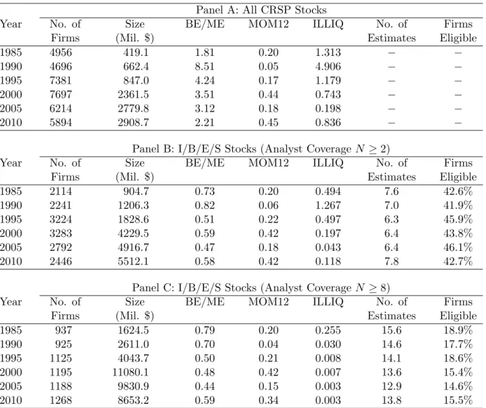
Table 1.1 provides a comparison of characteristics of all the stocks listed on CRSP (shown in Panel A), the firms that have a current-fiscal-year I/B/E/S earnings forecast and are covered by at least two analysts (shown in Panel B), and firms covered by at least eight analysts (shown in Panel C) in di↵erent years. Book-to-market ratio is defined following Fama and French (1993). We exclude stocks with negative book values, and with book-to-market ratio outside 0.5th and 99.5th percentile. Momentum is defined as the past raw return over t 12 to t 2 months. Illiquidity is defined as the average ratio of the daily absolute return (in percent) to the (dollar) trading volume on that day during the month t, the same as in Amihud (2002).
A large portion of the firms with I/B/E/S earnings forecasts are covered by a small number of analysts each month. As shown in Panel B, about 40% of the stocks are included in the sample when analyst coverage is at least two, and the percentage decreases to 15% - 19% when we limit our sample to stocks with at least eight analysts’ forecasts (see Panel C). While the mean book-to-market ratio and momentum are statistically indi↵erent for the three samples, the mean size of the stocks in Panel B is more than twice as large as the mean size of all stocks in CRSP and increases with analyst coverage. The mean illiquidity of stocks in Panel B is only about 1/3 of the mean illiquidity of all CRSP stocks, and decreases even further with the increase of analyst coverage. These results are consistent with the findings in the literature (e.g., Hong, Lim, and Stein (2000), Diether, Malloy, and Scherbina (2002), and Anderson, Ghysels, and Juergens (2005)) that I/B/E/S dataset is severely tilted towards large and liquid stocks.
8To overcome the first possibility, we also measure the heterogeneity of beliefs among analysts using the average of
1.3
Using Dispersion and Skewness in Beliefs to Forecast Returns
In this section, we examine whether the dispersion and skewness of analysts’ earnings forecasts have forecasting power for the subsequent returns of the underlying stock.
1.3.1 Portfolio Sorts Based on Dispersion
Before investigating the role of asymmetry of analysts’ earnings forecasts, we first reexamine the dispersion e↵ect documented in Diether, Malloy, and Scherbina (2002) using an extended sample period and a variety of analyst coverge cuto↵s. In each month t, stocks are sorted into quintile portfolios based on the dispersion in analysts’ earnings forecasts for the previous month. Stocks with a zero mean forecast are allocated to the highest dispersion quintile (D5). Stocks are held for one month. The monthly portfolio return is calculated as the equally-weighted returns of all the stocks in that portfolio.
The last column of Panel A in Table 1.2 shows the average of monthly returns of all the stocks in each dispersion quintile. During the extended sample period (1983 - 2012), the dispersion e↵ect is still significant. The monthly return on the D1 D5 strategy is 0.58%.9
Then we examine the mean returns of double-sorted portfolios formed on size and dispersion of analysts’ earnings forecasts. In each montht, stocks are sorted into quintile portfolios based on the market capitalization at the end of the previous month. Then stocks are sorted into quintiles relative to other stocks in their size quintile on the basis of dispersion in analysts’ earnings forecasts for the previous month. Table 1.2 reports the average of monthly portfolio returns for the 25 size-dispersion portfolios for two samples. The size-dispersion e↵ect is most pronounced for the smallest stocks. This results are consistent with the findings in Diether, Malloy, and Scherbina (2002). Considering that the stocks with high analyst coverage are mostly large stocks, stocks in small-cap quintiles are not actually small. So it is not surprising to find that for the stocks covered by eight or more analysts, the return di↵erential between low- and high-dispersion quintile decreases to 0.27% per month and is not statistically significant (see Panel B).
To assess how the dispersion e↵ect changes with the increase of anlayst coverage cuto↵, we compute average monthly returns on each dispersion quintile portfolios, as well as on theD1 D5
9Diether, Malloy, and Scherbina (2002) document a monthly return of 0.79% on theD1 D5 strategy for the sample
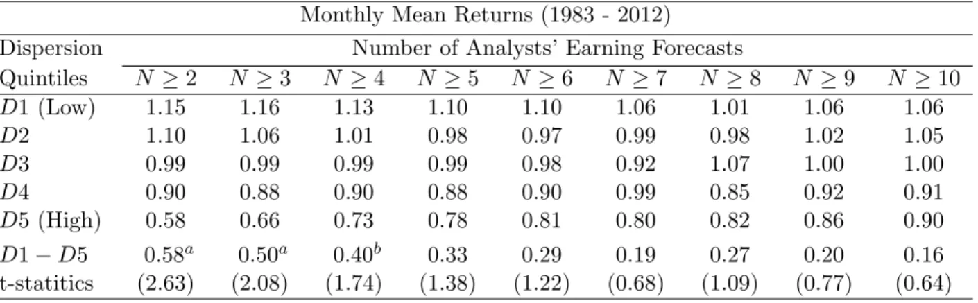
strategy for all the stocks with two or more analysts, three or more analysts, and up to ten or more analysts. Table 1.3 shows thatD1 D5 spread declines with the increase of analyst coverage cuto↵, and becomes insignificant for the sample of stocks that are covered by four or more analysts.
The measure issue is not negligible when one uses the sample of stocks that are covered by two or more analysts. As we discussed earlier, the cross-analyst estimate of dispersion is vulnerable to extreme observations. With merely two or three observations, this estimate could be inaccurate. Unfortunately, however, more than half of the stocks usually have low analyst coverage.10
Based on the implication of our model, the dispersion of opinion has opposite e↵ect on the stocks with negative skewness in beliefs, and on the stocks with positive skewness in beliefs. Without controlling for the skewness of agents’ beliefs, the dispersion e↵ect may be cancelled out. In next subsection, we will verify this argument and test three hypotheses postulated in Section 2.2.
1.3.2 Double Sorts Based on Dispersion and Skewness
First, we examine the relation between dispersion and skewness of analysts’ earnings forecasts and subsequent returns using double sorting method. In each month t, stocks are independently assigned into quintile portfolios on the basis of the dispersion and skewness of analysts’ earnings forecasts for the previous month. We then form portfolios based on the intersection of rankings of dispersion and skewness. Stocks are held for one month. The monthly portfolio return is computed as the equally-weighted returns of all the stocks in the portfolio at the end of month t+ 1. The monthly mean returns of the 25 dispersion-skewness portfolios are reported in Panel A of Table 1.4. “All stocks” row in Panel A reports the average monthly returns of dispersion quintile portfolios. The lowest-dispersion portfolio (D1) outperforms the highest-dispersion portfolio (D5) by 0.19% on average, positive but statistically insignificant. Now we read across the monthly returns of double-sorted portfolios. With respect to our first hypothesis, we find that within the portfolio with most negative skewness (Q1), the dispersion of analysts’ earnings forecasts has a strong negative relation with subsequent returns, and theD1 D5 strategy earns as much as 0.65% per month on average. With respect to our second hypothis, the return di↵erential between the lowest and highest quintiles of dispersion is virtually zero (0.04%) for the stocks within the most positive quintile of skewness
(Q5).
In Panel B of Table 1.4, the top and bottom dispersion quintiles D1 and D5 are further sub-divided into halves on the same measure. Within the most-negative-skewness portfolio (Q1), the monthly return on D1L D5H strategy is further amplifed to 0.97%. Within the most-positive-skewness portfolio (Q5), on the contrary, the relation between dispersion of analysts’ forecasts and portfolio returns is reversed. The monthly return onD1L D5H strategy is 0.57% and statistically significant at ten percent level. Note that after subdividing the dispersion quintiles into halves, four portfolios with extreme dispersion and skewness (D1LQ1,D1HQ1,D1LQ5 andD1HQ5) only contain 14-15 stocks on average and the results in Panel B are likely to be unreliable and not robust. This finding seems to be consistent with our Hypothesis 2. In the presence of short-sales constraints for some of the stocks will diminish the overall e↵ect of dispersion in analysts’ forecasts for the stocks with positively skewed beliefs.
With respect to Hypothsis 3, we look at the return di↵erential between the most-positive- (Q5) and most-negative-skewness (Q1) portfolios. As shown in the “All stocks” column of Panel A, the skewness of analysts’ earnings forecasts is positively related to the subsequent returns. The return di↵erential between top and bottom skewness portfolios is is 0.59% per month, statistically significant only within the highest dispersion quintile (D1).
1.3.3 Firm Characteristics of Dispersion-Skewness Portfolios
In our theoretical model, we assume that the source of heterogeneous beliefs is exogeneous, and in-dependent of the e↵ects of dispersion and skewness of agents’ beliefs. In reality, however, the degree of dispersion and asymmetry of heterogeneous beliefs may generically vary with stock character-isitcs. For example, many papers address private information as a possible source of heterogeneous beliefs, and information uncertainty is correlated with stock characteristics, such as size, book-to-market, momentum (Easley, Hvidkjaer, and Ohara (2002), and Zhang (2006)), illiquidity (Sadka and Scherbina (2007)), and analyst coverage (Hong, Lim, and Stein (2000)).
costs associated with the portfolio rebalancing.
In each month t, we calculate cross-sectional mean of size, book-to-market ratio, momentum, illiquidity, earings-to-price ratio and anlayst coverage of all the stocks in each dispersion-skewness portfolio. Table 1.5 reports the equally-weighted average of these variables and turnover rate for each of the 25 dispersion-skewness portfolios over the sample period. There are large cross-sectional variations in all the variables across the dispersion-skewness portfolios, except the number of estimates. The heterogeneity of the stock characteristics is more substantial among dispersion portfolios than the heterogeneity among skewness portfolios.
Turnover rates are high for most dispersion-skewness portfolios and exhibit seasonal patterns. Turnover rates are usually over 90% in January, and much lower during the other months of the year. It is not surpricing, since the fiscal year end for most stocks is December, and analysts start to forecast new fiscal-year earnings in January. Therefore, the distribution of analysts’ earnings forecasts of an individual stock in January could be substantially di↵erent from the distribution in last December. When we compute time-series means of turnover rates, January is excluded. Four portfolios of extreme dispersion and skewness (Q1D1, Q1D5, Q5D1, Q5D5) – ones that we are most interested in – have the lowest turnover rates. It seems that analysts with overly optimistic or pessimistic forecasts tend to revise their opinions less frequently. One plausible explanation is that as we have mentioned in section 2.2, high quality analysts have more confidence in their estimates and are less likely to herd.
Next, we test whether the di↵erences of these stock characteristics are significant between the lowest- and highest-dispersion portfolios, and between the most-negative- and most-positive-skewness portfolios. Table 1.6 reports equally-weighted average of stock characteristics11 of five dispersion portfolios in the top and bottom skewness quintiles.
The stocks with low consensus forecasts, small size, high book-to-market ratio, low returns over past 12 months, less liquidity, and less past year earnings tend to have more dispersion in analysts’ beliefs. And the stocks with low consensus forecasts, small size, high book-to-market ratio tend to have more positive skewness in analysts’ beliefs. The magnitude of t-statistics shows that the divergence in the stock characteristics is more substantial across dispersion quintiles than
11We take logarithm of size and book-to-market ratio to deal with the non-normality issue in these variables. We
the divergence across skewness quintiles. Moreover, the relations between the dispersion of ana-lysts’ earnings forecasts and these variables are very similar within the top and bottom skewness portfolios.
1.3.4 Triple Sorts
To verify that the documented dispersion and skewness e↵ects are not simply capturing a size, value, momentum, illiquidity or average forecasts e↵ect, now we examine the relation between dispersion and skewness of analysts’ earnings forecasts and subsequent returns while controlling for the variation in these variable, using triple sorts.
Average of analysts’ earnings forecasts. In each month t, stocks are independently sorted
into terciles on the basis of mean, dispersion and skewness of analysts’ earnings forecasts for the previous month. Then we assign stocks into portfolios based on the intersection of rankings of mean, dispersion and skewness. Terciles are based on 30th and 70th percentiles. The average monthly returns of the resulting 27 portfolios are reported in Table 1.7.
Within each average tercile, we continue to find negative relation between dispersion of analyts’ earnings forecasts and subsequent returns in the most negative skewness tercile. In low- and mid-average terciles, this relation is statistically significant. The skewness e↵ect is significant in mid-average tercile.12 The result rules out the possibility that the average of forecasts is driving our results.
Size. In each montht, stocks are independently sorted into tercile portfolios based on the level mar-ket capitalization at the end of the previous month, dispersion and skewness of analysts’ earnings forecasts for the previous month. We then assign stocks into portfolios based on the intersection of rankings of size, dispersion and skewness. Panel A in Table 1.8 reports the average monthly returns on the 27 portfolios. In three size terciles, D1 D3 stragegy remains to generate the highest and positive returns within the most-negative-skewness tercile, and the returns are most significant for the smallest tercile.
Book-to-market. Stocks are triple sorted based on book-to-market ratio, dispersion and skewness
12After triple sorts, the number of stocks in each resulting portfolio decreases. Moreover, the return di↵erential
in analysts’ forecasts. Panel B in Table 1.8 reports the average monthly returns on the resulting 27 portfolios. Within each book-to-market tercile, dispersion of analysts’ earnings forecasts and subsequent returns in the most-negative-skewness tercile still have negative relation. For stocks in growth tercile,D1 D3 stragegy has as much as 0.73% monthly returns on average. This is consis-tent with our intuition that with higher market-to-book ratio (growth stocks), more disagreement in earnings should result in more disagreemnt in market values.
Momentum. Stocks are triple sorted based on momentum, dispersion and skewness in analysts’
forecasts. Panel A in Table 1.9 reports the average monthly returns on the resulting 27 portfolios. Again the return di↵erential between low- and high-dispersion teciles is still the highest within the negative-skewness stocks for each of the momentum portfolio, and is significant in stocks that have performed poorly in the past 12 months (“Loser” and “Mid Mom”). So the dispersion and skewness e↵ects are not simply capturing a momentum e↵ect documented in Jegadeesh and Titman (1993).
Illiquidity. Stocks are triple sorted based on illiquidity, dispersion and skewness in analysts’ forecasts. Panel B in Table 1.9 reports the average monthly returns on the resulting 27 portfolios. The return di↵erential between low- and high-dispersion teciles within the negative-skewness tecile is significantly positive in most illiquid stocks (0.54% per month). Therefore, the dispersion and skewness e↵ects cannot be explained by illliquidity e↵ect. This result is also consistent with the argument in Sadka and Scherbina (2007) that illiquid stocks have higher transaction costs and hence the dispersion e↵ect is amplified.
1.3.5 Four-Factor Model Time-Series Tests
tercile portfolio, and represents the value premium.13 Carhart (1997) constructs a momentum factor that cannot be explained by Fama-French three-factor model. It captures the one-year momentum e↵ect documented in Jegadeesh and Titman (1993). Momentum factor UMD is the average return di↵erential between the tercile portfolio of stocks with high returns from montht 12 tot 2 and the portfolio of stocks with low returns from montht 12 tot 2, and represents the momentum premium.
For each of the 25 dispersion-skewness portfolios, we regress monthly equally-weighted average returns of the portfolio on Fama-French three factors and momentum factor,
Ri,t Rf,t=↵i+ i,m(Rm,t Rf,t) + i,sSMBt+ i,hHMLt+ i,uUMDt+"i,t.
If the portfolio excess returns can be explained by the four factors, intercepts from above time-series regressions should be jointly equal to zero. Then our main testable hypothesis is that↵i = 0 for all 25 dispersion-skewness portfolios. The Hotellingt2 test, introduced by Gibbons, Ross, and Shanken (1989), is used to test the hypothesis. A test statistic of 15.8 strongly rejects the null hypothesis and suggests that the dispersion and skewness of analysts’ forecasts have predictive power for future returns that is not captured by the standard predictors.
Table 1.10 reports the estimates of the four-factor time-series regressions for 25 dispersion-skewness portfolios. First, we look at the estimated coefficients of the four-factor regressions for 5 dispersion portfolios within each skewness quintile. The magnitude of the intercepts from the four-factor model are negatively related to the degree of dispersion in analysts’ earnings forecasts, which implies that low-dispersion portfolios earn more higher abnormal returns. In particular, the intercepts of all the highest-dispersion quintiles (D1), expect the one in the most-positive-skewness quintile, are significantly negative. Therefore, a large negative return for the portolio cannot be explained by the four factors. The loadings of the four factors are very di↵erent pattern across dispersion quintiles. Specifically, the loadings of SMB, HML and UMD factors in the lowest-dispersion quintiles (D1) have opposite signs compared with the loadings of three factors in high dispersion quintiles (D4 and D5). The lowest-dispersion portfolio behaves like a big, value and good past performance stock, and highest-dispersion portfolio behaves like a small, growth and bad
past performance stock. Results are consistent with the findings in Table 1.6.
Second, we compare the intercepts from the four-factor model for the negative- and most-positive-skewness quintiles. Intercepts of the 5 dispersion portfolios within the most-negative-skewness quintile are uniformly smaller than the intercepts within the most-positive-most-negative-skewness quin-tile, which indicates that positive-skewness portfolios earn more higher abnormal returns.
Adjusted R2s are lowest for the lowest-dispersion portfolios (D1), suggesting that four factors
have less explanatory power in stocks with low dispersion in analysts’ earnings forecasts. Overall, both GRS test and the magnitude of intercepts from four-factor time-series regressions confirm that the dispersion and skewness e↵ects documented in Section 4.2 cannot be captured by other traditional pricing factors.
1.4
Robustness Checks
We conduct a range of additional tests to ascertain the robustness of our basic results.
1.4.1 Subperiod Analysis
First, we redo the analysis using sample subperiod from January 1983 to December 2000 to compare our results with Diether, Malloy, and Scherbina (2002). Moreover, the subperiod analysis excludes the recent financial crisis of 2007-2009. During this period, many stocks have extremely negative earnings forecasts which tangle with other abnormally behaving factors. Panel A in Table 1.11 confirms that our main results are not time-specific.
In the most-negative-skewness portfolio (Q1), future returns are decreasing with the degree of dispersion and the monthly return on D1 D5 strategy is 1.06% on average, about 0.4% larger than the returns using the entire sample period. In the most-positive-skewness portfolio, monthly return onD1 D5 strategy declines to 0.34%, not statistically significant. For the skewness e↵ect, Q5 Q1 spread is 0.78% in high-dispersion portfolio, also larger than the returns using the entire
sample period.
1.4.2 Di↵erent Analyst Coverage Cuto↵
ranging from at least five analysts to at least ten analysts. Panel B in Table 1.11 reports the monthly mean returns of portfolios formed on dispersion and skewness of analysts’ forecasts for all the stocks that are covered by at leastten analysts. All the results remain virtually unchanged.
1.4.3 Portfolio Updating Frequency and Holding Period
As discussed earlier, analysts sometimes do not update their earnings forecasts regularly every month. To adjust for the staleness issue in analysts’ forecasts data, rather than forming portfolios based on the dispersion and skewness in the previous month, we form portfolios based on the average of dispersion and skewness in the past 3 or 6 months, and update portfolios every quarter or every six months. To consider the persistence of the dispersion and skewness e↵ects, we also try longer holding periods, from 3 to 6 months.
In the dissertation, we report two of these robustness analysis.14 Panel A of Table 1.12 reports
the results when we update portfolios at the end of the second month of each quarter (February, May, August and November) and hold portfolios for three months.15 D1 D5 stragegy has a significantly positive return (0.67% per month on average) only in the portfolio with most negatively skewed analysts’ earnings forecasts. Q5 Q1 stragety earns as large as 0.52% returns per month in the highest-dispersion quintile.
Panel B reports the results when we update portfolios semiannually (at the end of May and November) and hold them for 6 months.16 D1 D5 spread in the most-negative-skewness quintile
is slightly lower (0.59% per month) but still statistically significant . However, Q5 Q1 spread is no longer significant within any of the dispersion portfolio. It seems that the e↵ect of dispersion in analysts’ earnings forecasts is more persistent than the skewness e↵ect.
1.5
Additional Discussions
In this section, we discuss several additional topics with respect to our measure of heterogeneous beliefs.
14Results of other analysis are available upon request.
15We also try to update the portfolio at the end of the first or third month of each quarter, and results are similar.
1.5.1 Comparison with Stock Recommendations
Analysts provide both earnings forecasts and buy/sell recommendations of a stock. A natural ques-tion then arises: For any given stock, is there any relaques-tion between the dispersion and asymmetry of analysts’ earnings forecasts and the dispersion and asymmetry of their recommendations?
In I/B/E/S dataset, a stock with earnings forecasts also has data on analysts’ buy/sell recom-mendations, though it is not necessarily the case that two sets of analysts are the same. Intuitively, if the same set of analysts provide both earnings forecasts and recommendations of a stock at each point in time, and if analysts’ recommendations are “rationally” based on their perceived stock valuations – whenever an analyst has an optimistic valuation, she gives a “buy” recommendation decision, and vice versa – then the distribution of earnings forecasts should be comparable to the frequency distribution of stock recommendations. However, an extensive literature (e.g., Womack (1996), Ljungqvist, Marston, Starks, Wei, and Yan (2007)) have found that analysts are biased in stock recommendation. Unless analysts have extremely negative earnings forecasts in a stock, they are reluctant to provide a “sell” recommendation. Accordingly, we expect to detect a dispersion e↵ect using the stock recommdation data, which probably does not depend on the asymmetry of analysts’ recommendations – stocks with high dispersion in analysts’ earnings forecasts should also have more “sell” recommendations than the stocks with low dispersion have.
(D1).
1.5.2 Comparison with Ex Ante Variance and Skewness
We examine the relation between our dispersion and skewness of conditional expectation of future dividend and other measures of volatility and skewness. Bakshi, Kapadia, and Madan (2003) propose a method to calculate ex ante variance and skewness under risk-neutral probability. Conrad, Dittmar, and Ghysels (2013) find a negative relation between an individual securities risk neutral volatility and subsequent returns; more negative (positive) ex ante skewness predicts subsequent higher (lower) returns.
Panel A of Table 1.14 reports the mean ex ante variance of the 25 portfolios formed on the basis of dispersion and skewness of analysts’ earnings forecasts. Panel B reports the mean ex ante skewness of each portfolio. There is significantly positive relation between dispersion in analysts’ earnings forecasts and ex ante variance. Ex ante skewness is negative on average, and low dispersion in beliefs is associated with more negative ex ante skewness on average. Positive skewness in earnings forecasts is associated with less negative ex ante skewness on average, but the relation is not statistically significant.
However, our measure of dispersion and skewness of agents’ beliefs and ex ante volatility and skewness of stock returns predict subsequent returns in an opposite direction. This result confirms that the dispersion and skewness in analysts’ forecasts cannot be interpreted as a measure of risk.
1.6
Concluding Remarks
the stocks with high dispersion in agents’ beliefs. Empirical evidence is consistent with model implications. Both dispersion and skewness of analysts’ earnings forecasts have predictive power for subsequent returns, and the e↵ects remain even after controlling for the average of forecasts and standard pricing factors.
Table 1.1: Summary Statistics
The sample includes stocks from the NYSE, AMEX, and Nasdaq stocks between January 1983 and December 2012. Panel A reports descriptive statistics for all stocks listed on CRSP that have prices greater than five dollars. Panel B includes stocks in Panel A that have a current-fiscal-year I/B/E/S earnings forecast, are covered by at least two analysts. Panel C limits the sample to stocks in Panel B and are covered by at least eight analysts. Size is the market capitalization measured at the end of month t. BE/ME is the book-to-market ratio at the end of montht. MOM12 is the momentum of the stock, measured as the past raw return over t 12 to t 2 months. ILLIQ is the illiquidity of the stock, defined as the average ratio of the daily absolute return (in percent) to the (dollar) trading volume on that day during month t. Number of estimates is the number of analysts (denoted by N) who provide current-fiscal-year I/B/E/S earnings forecasts during month t. Column “Firm Eligible” reports the ratio of total number of stocks in Panel A (B) to the number of stocks listed on CRSP in a given year.
Panel A: All CRSP Stocks
Year No. of Size BE/ME MOM12 ILLIQ No. of Firms
Firms (Mil. $) Estimates Eligible
1985 4956 419.1 1.81 0.20 1.313
1990 4696 662.4 8.51 0.05 4.906
1995 7381 847.0 4.24 0.17 1.179
2000 7697 2361.5 3.51 0.44 0.743
2005 6214 2779.8 3.12 0.18 0.198
2010 5894 2908.7 2.21 0.45 0.836
Panel B: I/B/E/S Stocks (Analyst CoverageN 2)
Year No. of Size BE/ME MOM12 ILLIQ No. of Firms
Firms (Mil. $) Estimates Eligible
1985 2114 904.7 0.73 0.20 0.494 7.6 42.6%
1990 2241 1206.3 0.82 0.06 1.267 7.0 41.9%
1995 3224 1828.6 0.51 0.22 0.497 6.3 45.9%
2000 3283 4229.5 0.59 0.42 0.197 6.4 43.8%
2005 2792 4916.7 0.47 0.18 0.043 6.4 46.1%
2010 2446 5512.1 0.58 0.42 0.118 7.8 42.7%
Panel C: I/B/E/S Stocks (Analyst Coverage N 8)
Year No. of Size BE/ME MOM12 ILLIQ No. of Firms
Firms (Mil. $) Estimates Eligible
1985 937 1624.5 0.79 0.20 0.255 15.6 18.9%
1990 925 2611.0 0.70 0.04 0.030 14.6 17.7%
1995 1125 4043.7 0.50 0.21 0.008 14.1 18.6%
2000 1195 11080.1 0.48 0.42 0.007 13.6 15.4%
2005 1188 9830.9 0.44 0.15 0.003 12.9 14.6%
Table 1.2: Returns of Portfolios Formed on Size and Dispersion
The sample in Panel A includes stocks from the NYSE, AMEX, and Nasdaq, that have current-fiscal-year I/B/E/S earnings forecast between January 1983 and December 2012, and are covered by at least two analysts. Panel B limits the sample to stocks in Panel A that are covered by at least eight analysts. In each montht, stocks are sorted into quintile portfolios based on the market capitalization at the end of the previous month. Then stocks are sorted into quintiles relative to other stocks in their size quintile on the basis of dispersion of analysts’ earnings forecasts for the previous month. We then assign stocks into portfolios based on the intersection of rankings of size and skewness. Dispersion is defined as the standard deviation of analysts’ current-fiscal-year earnings per share forecasts scaled by the absolute value of the average of forecasts. Stocks with a zero mean forecast are allocated to the highest dispersion quintile (D5). Stocks are held for one month. The table presents the average monthly equally-weighted returns of 25 size-dispersion portfolios, along with return di↵erential of portfolios in dispersion quintile 1 and 5, D1 D5. t-statistics in parentheses are adjusted for serial-correlation using a Newey-West estimator with lags of up to 6 months.
Panel A: Monthly Mean Returns (1983 - 2012, Analyst Coverage 2) Size Quintiles
Dispersion S1 S2 S3 S4 S5
All Stocks
Quintiles (Small) (Large)
D1 (Low) 1.35 1.25 1.16 1.00 1.01 1.15
D2 1.35 1.11 1.11 0.95 0.99 1.10
D3 0.85 1.09 1.13 0.88 1.02 0.99
D4 0.63 0.99 0.81 1.06 1.03 0.90
D5 (High) 0.14 0.55 0.68 0.77 0.74 0.58
D1 D5 1.22a 0.70a 0.47 0.23 0.27 0.58a
t-statitics (4.94) (2.24) (1.47) (0.70) (0.83) (2.63)
Panel B: Monthly Mean Returns (1983 - 2012, Analyst Coverage 8) Size Quintiles
Dispersion S1 S2 S3 S4 S5
All Stocks
Quintiles (Small) (Large)
D1 (Low) 1.25 1.12 1.05 0.99 1.04 1.09
D2 0.97 0.87 1.13 1.05 0.98 1.00
D3 0.88 0.76 1.14 1.08 0.86 0.94
D4 1.13 0.83 1.03 1.10 0.83 0.98
D5 (High) 0.54 0.98 0.89 0.77 0.91 0.82
D1 D5 0.71b 0.15 0.16 0.22 0.13 0.27
t-statitics (1.81) (0.36) (0.46) (0.63) (0.31) (1.09)
Table 1.3: Returns to Dispersion Strategies with Di↵erent Analyst Coverage
The sample includes stocks from the NYSE, AMEX, and Nasdaq, that have one (fiscal) year I/B/E/S earnings forecast between January 1983 and December 2012. In each column, the sample is limited to stocks that are covered by from at least two analysts, up to at least ten analysts. Stocks with a price less than five dollars are excluded. In each month t, stocks are sorted into quintile portfolios on the basis of dispersion of analysts’ earnings forecasts for the previous month. Stocks with a zero mean forecast are allocated to the highest dispersion quintile (D5). Stocks are held for one month. The table presents the average monthly equally-weighted returns of 5 dispersion portfolios along with return di↵erential of portfolios in dispersion quintile 1 and 5, D1 D5, in samples with various thresholds of analyst coverage (N). t-statistics in parentheses are adjusted for serial-correlation using a Newey-West estimator with lags of up to 6 months.
Monthly Mean Returns (1983 - 2012)
Dispersion Number of Analysts’ Earning Forecasts
Quintiles N 2 N 3 N 4 N 5 N 6 N 7 N 8 N 9 N 10
D1 (Low) 1.15 1.16 1.13 1.10 1.10 1.06 1.01 1.06 1.06
D2 1.10 1.06 1.01 0.98 0.97 0.99 0.98 1.02 1.05
D3 0.99 0.99 0.99 0.99 0.98 0.92 1.07 1.00 1.00
D4 0.90 0.88 0.90 0.88 0.90 0.99 0.85 0.92 0.91
Table 1.4: Returns of Portfolios Formed on Dispersion and Skewness
The sample includes the NYSE, AMEX, and Nasdaq stocks that have a current-fiscal-year I/B/E/S earnings forecast, are covered by at least eight analysts, and have prices greater than five dollars. The sample period is from January 1983 to December 2012. The portfolio sorts in Panel A is as follows: in each month t, stocks are independently sorted into quintile portfolios based on the dispersion and skewness of analysts’ earnings forecasts for the previous month. We then assign stocks into portfolios based on the intersection of rankings of dispersion and skewness. In Panel B, dispersion quintiles 1 (D1) and 5 (D5) are further subdivided into halves on the same measure. We then assign stocks into portfolios based on the intersection of rankings of dispersion and skewness. Stocks are held for one month. Dispersion and skewness is defined as in Table 1.2. This table reports the average of monthly equally-weighted returns of each 25 dispersion-skewness portfolios, 5 dispersion portfolios (in “All stocks” row) and 5 skewness portfolios (in “All stocks” column). Panel A also reports return di↵erential of portfolios in dispersion quintile 1 and 5, and return di↵erential of portfolios in skewness quintile 5 and 1. Panel B reports return di↵erential of portfolios in two extreme dispersion deciles 1 (D1L) and 10 (D5H). t-statistics in parentheses are adjusted for serial-correlation using a Newey-West estimator with lags of up to 6 months.
PANEL A: Monthly Mean Returns (1983 - 2000, Analyst CoverageN 8) Dispersion Quintiles
Skewness D1 D2 D3 D4 D5 All D1 D5 t-stat
Quintiles (Low) (High) stocks
Q1 (Neg.) 1.05 0.80 0.99 0.91 0.40 0.85 0.65a (2.01)
Q2 0.91 1.10 0.94 0.90 0.86 0.93 0.06 (0.18)
Q3 0.93 0.85 1.14 0.78 1.10 0.95 0.17 ( 0.49)
Q4 1.12 0.92 1.15 0.65 0.84 0.93 0.29 (0.93)
Q5 (Pos.) 1.03 1.14 1.04 0.98 0.99 1.05 0.04 (0.13)
All Stocks 1.01 0.98 1.07 0.85 0.82 0.19 (0.68)
Q5 Q1 0.02 0.35b 0.06 0.08 0.59a 0.20a t-statitics ( 0.14) (1.76) (0.32) (0.42) (2.41) (1.96)
PANEL B: Monthly Mean Returns (Dispersion Deciles Dispersion Quintiles
Skewness D1 (Low) D3 D5 (High) All
D1L D5H t-stat
Quintiles D1L D1H D5L D5H Stocks
Q1 (Neg.) 1.26 0.88 0.99 0.50 0.30 0.85 0.97a (3.43)
Q2 0.91 0.92 0.94 0.95 0.76 0.93 0.15 (0.56)
Q3 1.02 0.84 1.14 1.15 1.04 0.95 0.01 ( 0.04)
Q4 1.12 1.05 1.15 0.78 0.87 0.93 0.25 (0.94)
Q5 (Pos.) 0.71 1.36 1.04 0.72 1.24 1.05 0.53a ( 1.75) Q5 Q1 0.56a 0.48b 0.06 0.23 0.94a 0.20a
t-statitics ( 2.09) (1.72) (0.32) (0.54) (2.10) (1.96)
Table 1.5: Characteristics of The Dispersion-Skewness Portfolios
The sample includes stocks from the NYSE, AMEX, and Nasdaq, that have one (fiscal) year I/B/E/S earnings forecast between January 1983 and December 2012, and are covered by at least eight analysts. The table reports equally-weighted average of stock characteristics for each dispersion-skewness portfolio over the sample period. In each montht, size, book-to-market ratio, momentum, illiquidity, earnings-to-price ratio, and number of estimates of a portfolio are computed as the equally-weighted mean of these variables for all stocks in a dispersion-skewness portfolio. Size, B/M, MOM12, ILLIQ and number of estimates are defined as in Table 1.1. E/P is the past year’s earnings per share divided by the price at the end of month t. Turnover rate of a portfolio in month tis the percentage of stocks remained in the same portfolio after the monthly updates. January is excluded when we compute mean turnover rate. t-statistics in parentheses are adjusted for serial-correlation using a Newey-West estimator with lags of up to 6 months.
Portfolio Avg Size B/M MOM12 ILLIQ E/P No. of Turnover
(Mil. $) Est. (%)
Q1D1 1.80 15808.5 0.41 0.20 0.94 10.10 14.1 47.0
Q1D2 1.95 11651.8 0.48 0.23 0.86 8.58 14.4 52.7
Q1D3 1.85 10778.8 0.51 0.26 0.87 6.91 14.5 52.5
Q1D4 1.64 7296.7 0.55 0.25 1.17 5.96 14.2 49.3
Q1D5 0.97 4037.5 0.67 0.14 1.37 0.68 13.7 44.5
Q2D1 1.87 13042.2 0.43 0.20 0.95 9.61 13.7 60.9
Q2D2 1.85 8279.1 0.52 0.21 1.01 7.39 13.6 65.9
Q2D3 1.88 8809.4 0.55 0.23 1.04 6.35 13.6 67.7
Q2D4 1.71 6921 0.60 0.25 1.04 5.15 13.7 66.8
Q2D5 0.78 3209 0.74 0.10 1.52 0.25 13.1 61.1
Q3D1 1.87 13098 0.44 0.20 0.96 10.03 13.7 63.6
Q3D2 1.88 8302.4 0.52 0.21 0.91 7.47 13.4 69.1
Q3D3 1.77 7880.7 0.56 0.18 1.04 6.29 13.5 70.5
Q3D4 1.66 6668.7 0.64 0.15 1.15 4.82 13.5 70.0
Q3D5 0.58 3208.1 0.79 0.07 1.61 1.00 13.2 66.0
Q4D1 1.97 14093.6 0.42 0.19 0.83 10.42 13.8 62.5
Q4D2 1.98 9447.1 0.50 0.19 0.85 8.21 13.5 66.7
Q4D3 1.74 8769.9 0.56 0.17 0.97 6.78 13.7 68.0
Q4D4 1.57 7547.9 0.64 0.12 1.34 5.30 13.4 67.4
Q4D5 0.54 3381.4 0.79 0.05 1.62 0.91 13.4 60.3
Q5D1 1.68 15436.3 0.40 0.19 0.90 9.82 14.2 47.9
Q5D2 1.82 11155 0.47 0.17 0.83 7.70 14.1 54.8
Q5D3 1.70 8843.4 0.52 0.15 0.88 6.95 14.1 54.7
Q5D4 1.34 7301.5 0.60 0.11 0.93 5.81 13.9 49.5
Table 1.6: Characteristics of The Dispersion-Skewness Portfolios (Cont0d)
The sample includes stocks from the NYSE, AMEX, and Nasdaq, that have one (fiscal) year I/B/E/S earnings forecast between January 1983 and December 2012, and are covered by at least eight analysts. The table reports equally-weighted average of stock characteristics of each dispersion portfolio in skewness quintile 1 and 5. In each panel, column “t(D1 D5)” reports the t-statistics of the di↵erences of mean variable between dispersion quintile 1 and 5; rows “t(Q5 Q1)” reports the t-statistics of the di↵erences of mean variable between skewness quintiles 5 and 1. ln(Size) is the logarithm of market capitalization at the end of month t. ln(BE/ME) is the logarithm of the book-to-market ratio at the end of month t. Momentum, illiquidity and earnings-to-price ratio are defined as in Table 1.5. In each month t, ln(Size), ln(BE/ME), momentum, illiquidity and earnings-to-price ratio of a portfolio are computed as the equally-weighted mean of these variables for all stocks in a dispersion-skewness portfolio. MOM12 is defined as the past raw return over t 12 to t 2 months. ILLIQ is defined as the average ratio of the daily absolute return to the (dollar) trading volume on that day during the montht. t-statistics in parentheses are adjusted for serial-correlation using a Newey-West estimator with lags of up to 6 months.
Skewness Dispersion Quintiles
Quintiles D1 D2 D3 D4 D5 t(D1 D5)
Mean Average of Analysts’ Forecasts
Q1 (Neg.) 1.95 2.01 1.85 1.62 0.95 (19.8)
Q5 (Pos.) 1.84 1.83 1.70 1.41 0.67 (24.3)
t(Q5 Q1) ( 4.96) ( 6.89) ( 5.98) ( 7.82) ( 8.85)
Mean ln(Size)
Q1 (Neg.) 8.42 8.16 7.98 7.70 7.28 (19.7)
Q5 (Pos.) 8.37 8.06 7.88 7.60 7.18 (19.7)
t(Q5 Q1) ( 1.73) ( 3.49) ( 3.85) ( 1.95) ( 1.95)
Mean ln(BE/ME)
Q1 (Neg.) 1.17 1.01 0.96 0.87 0.72 ( 22.3)
Q5 (Pos.) 1.15 1.01 0.90 0.77 0.61 ( 32.3)
t(Q5 Q1) (1.21) (0.10) (4.05) (7.46) (6.32)
Mean Momentum
Q1 (Neg.) 0.20 0.23 0.26 0.25 0.14 (4.2)
Q5 (Pos.) 0.19 0.17 0.15 0.11 0.01 (12.6)
t(Q5 Q1) ( 3.75) ( 5.79) ( 9.55) ( 11.7) ( 9.58)
Mean Illiquidity
Q1 (Neg.) 0.94 0.86 0.87 1.17 1.37 ( 2.9)
Q5 (Pos.) 0.90 0.83 0.88 0.93 1.50 ( 5.0)
t(Q5 Q1) ( 1.30) ( 0.14) (1.74) ( 1.26) (1.32)
Mean Earnings/Price
Q1 (Neg.) 14.6 13.4 12.9 8.26 4.50 (12.3)
Q5 (Pos.) 15.8 12.1 9.83 3.24 6.91 (9.4)
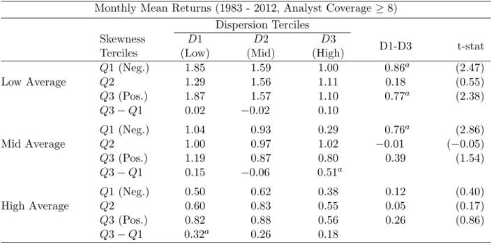
Table 1.7: Returns of Portfolios Formed on Average, Dispersion and Skewness
The sample includes the NYSE, AMEX, and Nasdaq stocks that have a one (fiscal) year I/B/E/S earnings forecast, are covered by at least eight analysts, and have prices greater than five dollars. The sample period is from January 1983 to December 2012. In each month t, stocks are inde-pendently sorted into terciles on the basis of mean, dispersion and skewness of analysts’ earnings forecasts for the previous month. Then we assign stocks into portfolios based on the intersection of rankings of mean, dispersion and skewness. Stocks with a zero mean forecast are allocated to the highest dispersion tercile (D3). Stocks are held for one month. This table reports the average of monthly equally-weighted returns of each of the 27 average-dispersion-skewness portfolios, along with return di↵erential of portfolios in dispersion tercile 1 and 3, D1 D3, and return di↵ eren-tial of portfolios in quintile tercile 3 and 1, Q3 Q1. t-statistics in parentheses are adjusted for serial-correlation using a Newey-West estimator with lags of up to 6 months.
Monthly Mean Returns (1983 - 2012, Analyst Coverage 8) Dispersion Terciles
Skewness D1 D2 D3
D1-D3 t-stat
Terciles (Low) (Mid) (High)
Low Average
Q1 (Neg.) 1.85 1.59 1.00 0.86a (2.47)
Q2 1.29 1.56 1.11 0.18 (0.55)
Q3 (Pos.) 1.87 1.57 1.10 0.77a (2.38)
Q3 Q1 0.02 0.02 0.10
Mid Average
Q1 (Neg.) 1.04 0.93 0.29 0.76a (2.86)
Q2 1.00 0.97 1.02 0.01 ( 0.05)
Q3 (Pos.) 1.19 0.87 0.80 0.39 (1.54)
Q3 Q1 0.15 0.06 0.51a
High Average
Q1 (Neg.) 0.50 0.62 0.38 0.12 (0.40)
Q2 0.60 0.83 0.55 0.05 (0.17)
Q3 (Pos.) 0.82 0.88 0.56 0.26 (0.86)
Q3 Q1 0.32a 0.26 0.18
Table 1.8: Returns of Triple-Sorted Portfolios: Size, Book-To-Market
The sample includes the NYSE, AMEX, and Nasdaq stocks that have a current-fiscal-year I/B/E/S earnings forecast, are covered by at least eight analysts, and have prices greater than five dollars. The sample period is from January 1983 to December 2012. Panel A reports the monthly mean returns of portfolios formed using size-dispersion-skewness triple sorts. In each montht, stocks are independently sorted into tercile portfolios based on the market capitalization at the end of the previous month, dispersion and skewness of analysts’ earnings forecasts for the previous month. We then assign stocks into portfolios based on the intersection of rankings of size, dispersion and skewness. Panel B reports the monthly mean returns of portfolios formed using B/M-dispersion-skewness triple sorts. In each montht, stocks are independently sorted into tercile portfolios based on book-to-market ratio at the end of the previous month, dispersion and skewness of analysts’ earnings forecasts for the previous month. We then assign stocks into portfolios based on the intersection of rankings of book-to-market ratio, dispersion and skewness. Stocks are held for one month. Portfolio return is calculated as the equally-weighted returns of all the stocks in that portfolio. t-statistics in parentheses are adjusted for serial-correlation using a Newey-West estimator with lags of up to 6 months.
Panel A: Triple Sorts on Size, Dispersion and Skewness Dispersion Terciles
Skewness D1 D2 D3
D1-D3 t-stat
Terciles (Low) (Mid) (High)
Small Cap Q1 (Neg.) 1.08 0.95 0.49 0.60a (2.19)
Q2 0.98 0.94 1.07 0.09 ( 0.32)
Q3 (Pos.) 1.21 1.03 0.81 0.40 (1.20)
Q3 Q1 0.12 0.08 0.32
Mid Cap Q1 (Neg.) 0.90 0.98 0.74 0.16 (0.54)
Q2 0.90 1.14 0.89 0.01 (0.04)
Q3 (Pos.) 1.12 1.04 1.02 0.10 (0.39)
Q3 Q1 0.23 0.06 0.28
Large Cap Q1 (Neg.) 0.96 0.95 0.58 0.38 (1.29)
Q2 0.89 1.03 0.77 0.11 (0.37)
Q3 (Pos.) 1.11 0.92 0.94 0.17 (0.63)
Q3 Q1 0.16 0.02 0.36b
Panel B: Triple Sorts on Book-to-Market, Dispersion and Skewness Dispersion Terciles
Skewness D1 D2 D3
D1-D3 t-stat
Terciles (Low) (Mid) (High)
Growth Q1 (Neg.) 0.97 0.96 0.24 0.73a (2.33)
Q2 0.87 1.18 1.11 0.24 ( 0.84)
Q3 (Pos.) 0.92 1.06 1.09 0.17 ( 0.59)
Q3 Q1 0.05 0.10 0.85a
Mid B/M Q1 (Neg.) 0.86 1.04 0.67 0.19 (1.00)
Q2 0.83 1.09 1.19 0.36 ( 1.74)
Q3 (Pos.) 1.17 0.91 1.14 0.03 (0.13)
Q3 Q1 0.32 0.12 0.47
Value Q1 (Neg.) 1.12 0.99 1.00 0.12 (0.54)
Q2 1.25 1.21 1.13 0.13 (0.58)
Q3 (Pos.) 1.59 1.33 1.24 0.35 (1.59)
Q3 Q1 0.47b 0.34 0.24