Sharif University of Technology
Scientia IranicaTransactions E: Industrial Engineering www.scientiairanica.com
A feedback-oriented data delay modeling in a dynamic
neural network for time series forecasting
M. Namakshenas, A. Amiri
and R. Sahraeian
Department of Industrial Engineering, Faculty of Engineering, Shahed University, Tehran, P.O. Box 18151-159, Iran. Received 13 August 2013; received in revised form 11 August 2014; accepted 13 April 2015
KEYWORDS Forecasting; Time series; Dynamic neural networks; Feedbacks.
Abstract. In this study, we develop a neural network with a time shifting approach to forecast time series patterns. We investigate the impact of dierent layer-weight congurations to capture the trends in seasonal, chaotic, etc. forms. We also hypothesize the combined eect of the delayed inputs and the forward connections to introduce a dynamical structure. The eect of overtting issue is procedurally monitored to gain the resistance property from the early stoppage of training process and to reduce the error of predictions. Finally, the performance of the proposed network is challenged by six well-known deterministic and non-deterministic time series and compared by the autoregression (AR), Articial Neural Network (ANN), Adaptive K-nearest Neighbors (AKN), and adaptive neural network (ADNN) models. The results show that the proposed network outperforms the conventional models, particularly in forecasting the chaotic and seasonal time series.
© 2016 Sharif University of Technology. All rights reserved.
1. Introduction and orientation
Neural Networks have shown to be eective in areas like forecasting, economy, bankruptcy prediction, risk assessment, nancial evaluation, and so on. The outputs of these predictions are used to take strategic decisions about the processes. Dierent statistical and technical tools have been historically used to predict the trends in time series and aid decisions to be made. Due to the criticality of these decisions, there are substantial interests in the modication and advancement of prediction methodologies.
Dierent types of neural network-based systems were employed in the past to predict dierent time se-ries. The main motivation behind the vast utilization of
*. Corresponding author. Tel.: +98 21 51212065; Fax: +98 21 51212021
E-mail addresses: [email protected] (M. Namakshenas); [email protected] (A. Amiri); [email protected] (R. Sahraeian)
neural networks is their non-parametric properties and data driven approximation of nonlinear functions [1,2]. In general, the architecture of networks is determined by using special heuristics [3]. The rst challenge in our study is to identify a robust and consolidated framework for our network.
Traditional methods like the polynomial estima-tion, spline, smoothing techniques, trigonometric ex-pansion, etc. make use of many parameters to achieve a convincible estimation of the process [4]. For example, consider the recognition of a trend using a conventional Fourier series method. If the length of available data is assumed to be 100, then it requires a high number of arithmetic calculations with a myriad of linear coecients. One of the main properties of a neural network is the ability to learn any complex relationships between input and output vectors, which is very dicult to be embodied in the conventional algorithmic methods [5,6].
There exist many novel trends towards the struc-tural modication of neural networks in the literature.
Many researchers implemented the adaptive forms of neural networks to forecast complex benchmarks (see, for example [3,5,7-13]). An adaptive network must self-adapt its structure and self-adjust its parameters over time as changes are sensed. Self-adaptation plays a central role in the dynamically changing environments. It is concerned with the capability of the system to responsively self-adjust upon occurrence of a change in the environment [10].
Unlike a static neural network, a dynamic neu-ral network employs extensive feedback between the neurons of a layer and/or between the layers of the network. This feedback implies that the network has also local memory characteristics. The node equations of a dynamic network are described by dierential equations. Since they contain the feedback paths from their outputs to the inputs, the response of a dynamic neural network is recursive; the local memories store the recursive information. For a stable network, successive iterations produce smaller output changes until the outputs eventually become constant [14].
Forecasting time series data patterns by the arti-cial neural networks has recently gained much interest as compared to the other methods. Researchers are almost unanimous that neural networks could be a very practical tool for analyzing time series forecasting mod-els. Traditional models like exponential smoothing, time series regression, autoregressive moving average, and splines are almost constructed on the linearity and the dependency premises. The real instances in many cases do not follow these suppositions; this would be a major drawback in detecting relationships by the analytical methods [15].
In the study by Zhang & Qi [6], an investigation was conducted based on the issue of how to eectively describe time series models in terms of both the seasonal and the trend patterns. In their study, the eectiveness of data preprocessing on the basis of forecasting performance and neural network modeling was queried, including deseasonalizing and detrending factors (for a brief introduction of these two elements, please see the next section). The prediction results were examined and compared to those acquired from the Box{Jenkins seasonal autoregressive moving aver-age models. The preponderance of evidence suggested that the neural networks were not capable of capturing the seasonal or trend variations, eectively, by feeding unpreprocessed raw data.
Kulesh et al. [7] made use of adaptive metrics to produce acceptable predictions. In the study, a special adjustment of the nearest neighborhood method is pro-posed in order to improve the accuracy of forecasting a time series. The modications are conducted according to the following schema: First, all dened subsets of time series are compared with the last subsets and then a subset is chosen, i.e. the closeness measure of
the last subset with other subsets is calculated [7,8]. Selection of the closeness function accounts for a major step in obtaining a good prediction accuracy. Note that closeness is dened in terms of the distance metric on the Euclidean space.
Khashei & Bijari [4] presented a novel hybrid framework of an articial neural network and an ARIMA model in order to overcome the restriction of ANNs in time series forecasting and to yield more accu-rate forecasting results than those of the conventional hybrid ARIMA-ANNs models. In their study, a linear ARIMA model is developed to recognize and magnify the linear structure in the dataset. Furthermore, a neural network model is constructed to capture the underlying data process by using the preprocessed data. The empirical results with three well-known real data sets are presented and the proposed model is compared with the traditional hybrid models.
Some other addressable research has challenged Dynamical Recurrent Neural Networks (DRNN) for time series forecasting (for example, see [16]). Since the recurrent synapses, connections, are represented by a \Filtering Impulse Response (FIR)", the DRNN is a state-based model in which all hidden layers obtain local memories like the state variables. The model is trained by a temporal recurrent backpropagation algorithm (TRBP); hence, exponential decay of the temporal reverse gradient is exploited for the training procedure with a minimal computational eort. Any economic DRNN model is capable of extracting the ap-propriate internal relationships between various chaotic processes from a subset of state variables [16]. We summarize important research, known to the authors, on forecasting by ANNs in Table 1.
In order to determine the best structure of the network, we use a framework of functions to generate the training, evaluation, and test sets. The framework is built on MATLAB software to customize the Neural Network Toolbox. Moreover, in order to evaluate the overall performance of the methodology, we will also compare it with the various forecasting models.
The rest of the paper is organized as follows: Section 2 introduces the structure and the development process of the proposed network. In Section 3, the pro-posed network is examined through 6 numerical bench-marks including deterministic and non-deterministic data patterns. Section 4 presents the analysis and comparison of the proposed model with the others via six time series data patterns. Our concluding remarks are presented in the nal section.
2. Proposed neural network
The node equations in dynamic networks are described by dierential equations. It is possible to develop a static network which processes time series data by
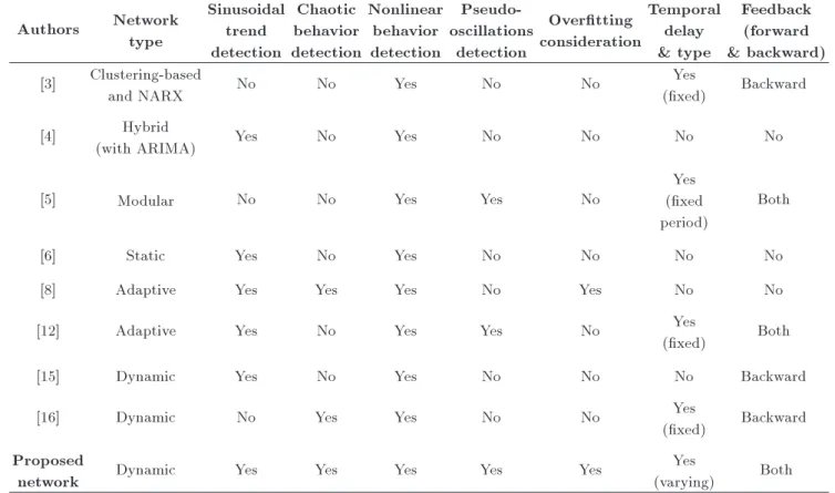
Table 1. Comparison based on forecasting features of various neural networks in the literature. Authors Network type Sinusoidal trend detection Chaotic behavior detection Nonlinear behavior detection Pseudo-oscillations detection Overtting consideration Temporal delay & type Feedback (forward & backward) [3] Clustering-based
and NARX No No Yes No No
Yes
(xed) Backward
[4] Hybrid
(with ARIMA) Yes No Yes No No No No
[5] Modular No No Yes Yes No
Yes (xed period)
Both
[6] Static Yes No Yes No No No No
[8] Adaptive Yes Yes Yes No Yes No No
[12] Adaptive Yes No Yes Yes No Yes
(xed) Both
[15] Dynamic Yes No Yes No No No Backward
[16] Dynamic No Yes Yes No No Yes
(xed) Backward Proposed
network Dynamic Yes Yes Yes Yes Yes
Yes
(varying) Both
simply converting the temporal connections into the dynamic patterns by assigning the sequence over a nite training period. The latter is processed by suspending some of the input sequences when feeding the network. This architecture is often seen as a Delay Neural Network (DNN) i.e. the DNN gains the dynamic behavior { delay { by means of backward connection.
In this study, a dynamic neural network with forward and backward with interactive data shifting approach is proposed. The delay concept enables the networks to recognize the trends and unusual patterns. Trends in time series are slow and make gradual changes in some properties of a series over the entire interval. Trends are sometimes loosely dened as the long term changes in the process mean. Moreover, detrending is a statistical or mathematical operation of removing trends from the series. On the other hand, what we might like to do is just removing the seasonal eect and leaving any trends and random ups and downs back in the data. The resulting series give us what is known as deseasonalized data, oscillations, which may give us a clearer picture of the patterns.
To illustrate the accuracy of the proposed net-work, several deterministic and chaotic time series and real observations are prepared. The Mean Absolute Percentage Error (MAPE) statistic is implemented to evaluate the prediction performance of the model. In the literature, MAPE is regarded as one of the standard statistical performance measures which is given in
Eq. (1):
MAPE(%) = 100M XM
i=1
yi ~yi
yi
; (1)
where yi is the source point, ~yi is the predicted point,
and M is the number of forecasted points. The Normalized Mean Square Error (NMSE) is also used as the error criterion [8], which is the ratio of the mean squared error to the variance of time series. It is dened by Eq. (2):
NMSE =
M
P
i=1(yi ~yi) 2 M
P
i=1(yi yi)
2; yi=
1 M
M
X
i=1
yi; (2)
where yi is the mean of observations in time series. It
is clear that resistance of the overtting issue requires the number of epochs for training the network to be small. In contrast, it should be large enough to train the network with any monotonous string of patterns.
We deploy the step by step strategy to construct a fully-connected network. The state-space diagram of the proposed network is illustrated in Figure 1. Exclud-ing input and output data elements, a three-hidden-layers network is used. Through empirical analyses, we suggest that T f1 (Transfer Function) and T f3 should
Figure 1. State-space diagram of the proposed network.
and a linear transfer function be employed in the intermediate hidden layer. A feedback connection is used from output of T f2 to L1W3 (layer-weight) for
detrending purpose and the connection between T f3
and L1W2 incorporates deseasonalizing concept. Also,
in order to detect the hidden oscillations, especially in the chaotic patterns, the output of T f3 is connected
to layer-weight L3W3 with the varying data pattern.
Also, we empirically experiment that the forward connections in forms of I1W1 to I3W1, I2W2 to I3W1,
and I1W1 to I2W1 marginally reduce the overtting
eect so that the rst form substantially accounts for the reduction. This connection is necessary for avoiding early stop of the training process. Further, we place temporal delay Dij before the layer-weights
and input-weights in order to appropriately detect the time series behaviors. The procedure constructs the proposed Dynamic Delayed Neural Network with Forward connections (DDNNF).
The proposed topology faces two types of the data either processed or unprocessed:
Present and past values of the inputs, I(t); I(t 1); ; I(t n + 1), which represent exogenous inputs;
Delayed values of the outputs, y(t), y(t 1); , y(t n + 1), on which the model output y(t + 1) is regressed.
We sketch out the procedure by presenting the tran-sitional equations for each state upon transferring the data from one module to another. Note that we are only interested in the delay form of the equations which aects the dynamicity. Since the delay pattern is variable, we use ~dij representing the delay form in
the corresponding layer. (In order to keep the state equations as simple as possible, we use conjunction symbol to represent the mixed forms of the outputs as processed data in the training phase.)
State 1: D11(I(t)) = I
t d~11
;
D12(y(t)) = y
t d~12
: State 2:
D31
It d~11
= It d~11 d~31
;
D33(y(t)) = y
t d~33
;
D13(!1) = !1
Tn d~13
: State 3:
!1(Tn) =
n
It d~11
; !1
Tn d~13)
;
yt d~12
o ;
D32(!1) = !1
Tn d~32
: State 4:
!2(Tn) =
n
It d~11 d~31
; !1
Tn d~32
;
yt d~33
o ;
D33(y(t)) = y
t d~33
:
where !i(Tn) is the amalgamated form of the input
values of the corresponding delayed module. ~d31, ~d32,
and ~d33are important delay parameters, because they
have explicit inuence on !2(Tn) and, consequently,
control the SSE (Sum Square Error) function.
Then, a static backpropagation algorithm based on error function in Eq. (3) can be applied:
SSE = X
Tn2t;t 1; ;t n+1
Table 2. Parameter conguration for simulation. Benchmark type
Total number of neurons in
all layers
Temporal suspension Seasonal dependence time series 26 2
High-frequency time series 20 2
Dung chaotic time series 15 Max(5)
Mackey-Glass chaotic time series 16 Max(5)
Sunspot time series 14 Max(6)
Trac time series 26 Max(7)
3. Numerical examples
In order to justify ecacy of the presented network, we compare it with Auto-Regression (AR), Articial Neural Network (ANN), Adaptive k-nearest Neighbors (AKN), and adaptive neural network (ADNN) models. The parameters of the AKN, ADNN, and AR(m) models are taken from the study of Wong et al. [8]. Our proposed network is analyzed by some well-known test beds in the literature. In this section, we generate six data patterns based on two deterministic and seasonal benchmarks with a certain amplitude and trend, two chaotic time series, and two sets of the real time series based on the observations and the newly recorded statistics with the signicant errors. Table 2 presents the benchmarks with the number of neurons in each layer of the network and the time delay value. Obviously, there exists no simple prescribed strategy to determine the number of neurons and the time delays; hence, we arbitrarily choose them by the try-and-error method. However, it is axiomatic that there is a classic correlation between the number of neurons and the size of feeding data.
3.1. Deterministic data pattern
The rst synthetic time series is characterized by the seasonal attributes like trend changes and linear increase:
TS1(t) = cos
t
sin
t 4
+40t +10; (4) where t is the time element in a range from 0 to 2200 and is the trend parameter with value of 10. As it was mentioned previously, the amplitude of the seasonal element does not vary assuming that the period of sinu-soidal signal is known in advance. A Fourier spectrum of the series identies the component frequencies in data processing. Clearly, a modulation phenomenon, which is the consequence of multiplication of two sinusoidal signals, exists in the data (Figure 2). The rst 2200 lengths are used for training, and the last 200 sources are reserved for prediction.
The simulation results show that the proposed model is able to predict this time series, accurately.
Figure 2. Time series with seasonal dependency (vertical line shows the prediction start) with error versus time plot.
Since the synthetic time series has a feature of extreme orderliness, the result of ADNN is not better than that of the AR model. However, DDNNF outperforms AR in both measures and it must be noticed that the static ANN is incapable of detrending, because its structure is vulnerable to the oscillations.
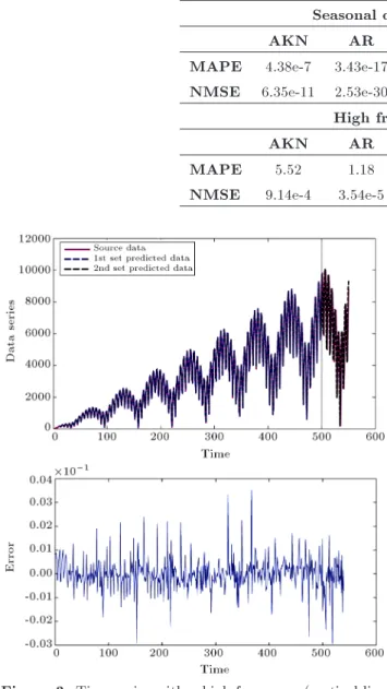
The second time series formulates a high-frequency dataset with a seasonal periodicity and smoothly increasing amplitude:
TS2(t) = 50t sin
t
+cos10t ; (5) where t is the time interval between 0 and 550 and parameter is equal to 2. The complexity of this synthetic series can be envisioned by plotting a Fourier spectrum. It is concluded that the interaction between the trends, amplitude, and seasonality renders this
Table 3. The summary of predictions of deterministic data patterns. Seasonal dependence data pattern
AKN AR ANN ADNN DDNNF
MAPE 4.38e-7 3.43e-17 0.02 3e-3 3.6495e-22 NMSE 6.35e-11 2.53e-30 1.16e-3 1.3e-10 2.4281e-43
High frequency data pattern
AKN AR ANN ADNN DDNNF
MAPE 5.52 1.18 1.09 1.17 0.7553
NMSE 9.14e-4 3.54e-5 7.01e-10 1.78e-4 4.1741e-15
Figure 3. Time series with a high-frequency (vertical line shows the prediction start) with error versus time plot.
benchmark dicult to be handled with standard neural network models (Figure 3). The rst 10/11 of the data is used for training the network and the rest is reserved for the prediction purpose.
According to Table 3, it can be claimed that DDNNF, which contributes to very small amounts in both measures, has the highest capability of de-trending and deseasonalizing. Also, Table 3 shows that the performance of ADNN is better than that of the ANN and AR models in terms of MAPE for which ANN scores the best prediction. Also, the performance of ADNN is closer to that of AKN in terms of NMSE, and the performance of AR and ANN is closer to that of ADNN with respect to MAPE. The above simulation results indicate that the ADNN model benets from the metrics provided by ANN and AKN.
3.2. Non-deterministic data pattern
In this section, we draw an explicit analogy between our proposed network and other models. The comparison is based on two chaotic time series data patterns and two observed datasets. The chaotic data patterns are generated from the Dung equation and the Mackey-Glass delay-dierential equation. It should be noted that these time series do not constitute any global amplitude or trends.
The rst non-deterministic time series we intro-duce is the Dung equation chaotic time series [8]. The generated data based on the system of dierential equations is given as follows (we use only the horizontal component of this series):
dy
dx = y + x x3+ cos(t); dy
dx = y: (6)
This system is characterized by two factors: the driving force and the damping phenomenon by which the chaotic behavior is determined. The amplitude parameter , frequency parameter , and parameter k are assumed to be 6, 1.33, and 0.1, respectively, to explicitly produce the chaotic behavior. Note that the resulting system of equations is dicult to be treated either analytically or numerically.
Instead, the medium order interactive Runge Kutta technique with the simulation-state method is employed to simulate the chaotic series (Figure 4). Table 4 indicates that the DDNNF has better per-formance than the AR and AKN models, and it has almost the same performance as that of ANN. This fact can be seen as a moderate capability of DDNNF at deseasonalizing the pattern. In this case, the ANN illustrates a surprising performance at detrending and detecting the chaotic pattern such that it outperforms other models in the NMSE measure.
The previous time series had some controllable chaotic characteristics, however, the chaotic behavior attributed to the Mackey-Glass equation is not known and dened to map the complex pattern to itself. The
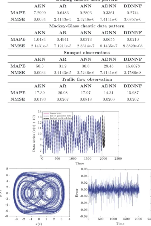
Table 4. The summary of predictions of data patterns and real observations Dung chaotic data pattern
AKN AR ANN ADNN DDNNF
MAPE 7.2999 0.6483 0.2806 0.3361 0.2744 NMSE 0.0034 2.4143e-5 2.5246e-6 7.4141e-6 3.6857e-6
Mackey-Glass chaotic data pattern
AKN AR ANN ADNN DDNNF
MAPE 1.0484 0.4941 0.0373 0.0655 0.0210 NMSE 2.1431e-3 7.1211e-5 2.8314e-7 8.1435e-7 9.3829e-08
Sunspot observations
AKN AR ANN ADNN DDNNF
MAPE 50.3 31.2 30.8 28.45 15.8078
NMSE 0.0034 2.4143e-5 2.5246e-6 7.4141e-6 3.7586e-8 Trac ow observation
AKN AR ANN ADNN DDNNF
MAPE 17.39 26.98 17.97 14.31 15.987
NMSE 0.0193 0.0267 0.0818 0.0206 0.0202
Figure 4. Chaotic time series of Dung equation (vertical line shows the prediction start) with trajectory and error versus time plot.
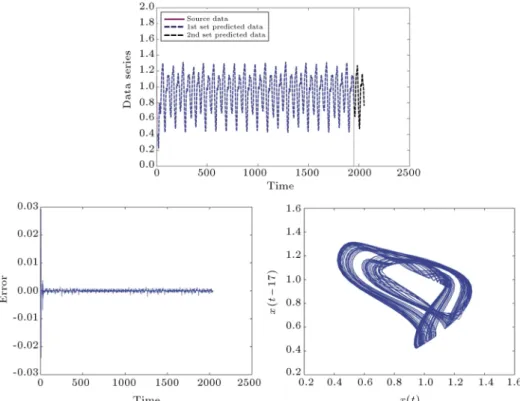
Mackey-Glass benchmark is known for its diculty in the evaluation by the state-of-the-art prediction methods [8]. The equation is given as follows:
dy(t)
dt = y(t) +
x(t )
1 + xc(t ); (7)
where = 17, c = 10, = 0:2 and = 0:1. The length of the data generated by this function is assumed to be 2050. The rst 95 percent of the time series length is
used for training the network. Note that the dataset is generated using the simulation-state method with a numerical simulator, as illustrated in Figure 5. Table 4 indicates that DDNNF almost outperforms all models in both measures. Table 4 also indicates that ADNN has almost the same performance as that of the new model and ANN.
In the literature, it is often seen that the networks which are competent at predicting the chaotic behavior often fail in the other data series collected from hourly,
Figure 5. Chaotic time series of Mackey-Glass delay dierential equation (vertical line shows the prediction start) with trajectory and error versus time plot.
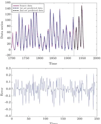
daily, weekly, monthly, and yearly observations, say real time series. It is a common practice to ascribe any well-suited patterns and trends to some natural phenomena inclined to estimable repetitions. How-ever, there exist some other events with unnatural trends, e.g., the sunspot dataset. This time series has been famous for a pseudo-period of 11 years, which is collected from the annual activities of the dark spot visible from the face perspective of the sun (Figure 6). The logic behind testing this dataset is that it is nonlinear; it cannot be tted by any statistical distributions, and the type of correlation is unknown; therefore, it has traditionally been used to examine the eectiveness of nonlinear and neural network models. In our study, we submit 221 points (1700-1920) for training the network and 35 points (1921-1956) for the forecasting purpose. The results suggest that DDNNF has the best quality in forecasting this benchmark in comparison with the other models. The results also imply that the overtting problem has been successfully treated in spite of a severe shortage of the test data.
The next and last real time data set is the trac ow data form an hourly vehicle counting observation for Monash Freeway, outside Melbourne, Australia. The dataset comprises 1690 observations during 11 weeks gathered in 1995 (the dataset is illustrated in Figure 7). The results show that our proposed model has a medium quality in comparison with the other models for this case. Regarding the MAPE measure,
ADNN scores the rst stage but in case of the NSME measure, AKN has the best performance among others. Again, the excellent capability of AR at detrending is obvious.
4. Conclusion
In this paper, we developed a network based on two aspects: the forward and backward connections for capturing dierent patterns and the time shift-ing inputs. Our explanation for why feed-backshift-ing helps is that the seasonal and trend variations of a time series might account for the convergence of its total variation. The models that ignore these seasonal or trend patterns will eventually result in a high variation with poor forecasting accuracy. The prediction results are examined and compared to those acquired from the Box{Jenkins seasonal autoregres-sive moving average models. The preponderance of evidence suggests that neural networks with un-shifted data are not capable of capturing seasonal or trend variations; either detrending or deseasonalizing techniques can drastically decline the prediction er-rors.
The ecacy of the presented network is validated by two sets of complex time series, say, the determin-istic and the non-determindetermin-istic time series including the chaotic time series and the real observations. In addition, the predicted results generated by DDNNF were also compared with those by the ADNN, ANN,
Figure 6. Real sunspots observation dataset (vertical line shows the prediction start) with error versus time plot.
Figure 7. Trac ow dataset (vertical line shows the prediction start) with error versus time plot.
AR, and AKN models. It was indicated that the proposed model outperforms these conventional tech-niques, particularly in forecasting chaotic and seasonal time series. Moreover, we found that by the empirical analyses, the forward connections in dynamic networks
with time delays have a signicant impact on the reduction of overtting issues.
Acknowledgment
The authors are grateful to an anonymous reviewer for precious comments which led to improvement in the paper.
References
1. Crone, S.F., Hibon, M. and Nikolopoulos, K. \Ad-vances in forecasting with neural networks? Empirical evidence from the NN3 competition on time series pre-diction", International Journal of Forecasting, 27(3), pp. 635-660 (2011).
2. Samarasinghe, S., Neural Networks for Applied Sci-ences and Engineering from Fundamentals to Complex Pattern Recognition, Taylor & Francis Group, NY (2007).
3. Soman, P.C. \An adaptive NARX neural network approach for nancial time series prediction", A Thesis submitted to the Graduate school - New Brunswick Rutgers, The State University of New Jersey (2008).
4. Khashei, M. and Bijari, M. \A novel hybridization of articial neural networks and ARIMA models for time series forecasting", Applied Soft Computing, 11(2), pp. 2664-2675 (2011).
5. Khotanzad, A., Hwang, R.-C., Abaye, A. and Maratukulam, D. \An adaptive modular articial neural network hourly load forecaster and its imple-mentation at electric utilities", IEEE Transactions on Power System, 10(3), pp. 1716-1722 (1995).
6. Zhang, G.P. and Qi, M. \Neural network forecasting for seasonal and trend time series", European Journal of Operational Research, 160(2), pp. 501-514 (2005).
7. Kulesh, M., Holschneider, M. and Kurennaya, K. \Adaptive metrics in the nearest neighbours method", Physica D, 237(3), pp. 283-291 (2008).
8. Wong, W., Xia, M. and Chu, W. \Adaptive neural network model for time-series forecasting", European Journal of Operational Research, 207(2), pp. 807-816 (2010).
9. Radulovic, J. and Rankovic, V. \Feedforward neural network and adaptive network-based fuzzy inference system in study of power lines", Expert Systems with Applications, 37(1), pp. 165-170 (2010).
10. Bouchachia, A. and Nedjah, N. \Adaptive incremental learning in neural networks: A review", Neurocomput-ing, 74(11), pp. 1783-1784 (2011).
11. Lee, E.W.M. \An incremental adaptive neural net-work model for online noisy data regression and its application to compartment re studies", Applied Soft Computing, 11(1), pp. 827-836 (2011).
12. Na, J., Ren, X., Shang, C. and Guo, Y. \Adaptive neural network predictive control for nonlinear pure
feedback systems with input delay", Journal of Process Control, 22(1), pp. 194-206 (2012).
13. Tianping, Z. and Qikun, S. \Novel design of adaptive neural network controller for a class of non-ane nonlinear systems", Communications in Nonlinear Sci-ence and Numerical Simulation, 17(3), pp. 1107-1116 (2012).
14. Sinha, N., Gupta, M. and Rao, D.H. \Dynamic neural networks: An overview", Industrial Technology, 2(1), pp. 491-496 (2000).
15. Ghiassia, M., Saidaneb, H. and Zimbrac, D.K. \A dynamic articial neural network model for forecasting time series events", International Journal of Forecast-ing, 21(2), pp. 341-362 (2005).
16. Aussem, A. \Dynamical recurrent neural networks to-wards prediction and modeling of dynamical systems", Neurocomputing, 28(1-3), pp. 207-232 (1999).
Biographies
Mohammad Namakshenas received BS and MSc degrees from the Department of Industrial Engineering at Payam Noor University of Tabriz Central and Shahed University, Iran, respectively. His research
in-terests include combinatorial optimization, simulation methods, and neural networks.
Amirhossein Amiri is an Associate Professor at Shahed University, Iran. He holds BS, MS, and PhD degrees in Industrial Engineering from Khajeh Nasir University of Technology, University of Science and Technology, and Tarbiat Modares University, Iran, respectively. His research interests include statistical quality control, prole monitoring, and Six Sigma. He has published many papers in the area of statistical process control in high quality international journals. He has also published a book with John Wiley and Sons in 2011, entitled Statistical Analysis of Prole Monitoring.
Rashed Sahraeian is an Associate Professor in the Department of Industrial Engineering at Shahed Uni-versity. He holds PhD in Industrial Engineering from Tarbiat Modares University. His research interests are scheduling and optimization in facility location prob-lem and supply chain management. He is author and co-author of several papers which have been published in Iranian and international journals.