Sharif University of Technology
Scientia IranicaTransactions E: Industrial Engineering www.scientiairanica.com
Integrated dynamic cell formation-production planning:
A new mathematical model
M. Rabbani
a;, S. Keyhanian
b, N. Manavizadeh
cand H. Farrokhi-Asl
d a. School of Industrial Engineering, College of Engineering, University of Tehran, Tehran, Iran.b. Department of Industrial Engineering and Management Systems, Amirkabir University of Technology, Tehran, Iran. c. Department of Industrial Engineering, Khatam University, Tehran, Iran.
d. School of Industrial Engineering, Iran University of Science & Technology, Tehran, Iran. Received 1 October 2015; received in revised form 14 April 2016; accepted 22 August 2016
KEYWORDS Dynamic cell formation;
Dynamic production planning;
Integrated
mathematical model; Lot splitting; Ant colony optimization.
Abstract. In this paper, a dynamic cell formation problem is presented considering some new and special characteristics. The concept of machine requirement by lucky parts, the parts which are allowed to be produced in a specic period, is combined with the depreciable property of machines. Therefore, purchasing and selling of machines according to their book-value and generating income have been taken into account. This leads to a new vantage characteristic in cell formation where, in each period, we deal only with the types and number of machines required. The new mathematical model is presented and solved by exact and ant colony optimization methods for three problem sizes.
© 2017 Sharif University of Technology. All rights reserved.
1. Introduction
In this paper, a dynamic cell formation problem is considered taking into account some new and special characteristics. Dierent types of machines are located in dierent cells with various types of parts which should be operated on them. Operation sequence has been considered under the concept of routes having dierent machines through them. Each type of parts has a set of routes consisting of machine sequences, which utilize the concept of exible routing used in literature [1-3]. Also, the concept of machine exibility is applied in order to provide the ability to perform one or more operations for each machine type [4,5]. By
*. Corresponding author. Tel.:+98 21 88021067; Fax: +98 21 88013102
E-mail addresses: [email protected] (M. Rabbani); [email protected] (S. Keyhanian );
[email protected] (N. Manavizadeh); [email protected] (H. Farrokhi-Asl) doi: 10.24200/sci.2017.4387
assuming that each part can only get operated in one route in each period, the number of parts of each type fully operated in each period and in each route forms a production lot of that part type, which aims to satisfy a known and deterministic demand of a specic period by getting added up to other periods' production lots of that part type (lot-splitting among periods and routes). Despite considering dynamicity, which allows relocation of machines and reconguration of cells, ma-chines' book-values decrease by depreciation and there is an allowance to purchase and sell machines in each period in the cell formation environment considered here. This is dierent from the concept of adding and removing machines; because, in this case, the system is charged with an income when removing machines and, thus, some negative statements appear in the objective function. Therefore, we seek to achieve the best combinational design of cells and machines and part routes in order to minimize the cost function of cell formation problem.
The rest of the paper is organized as follows. In Section 2, a comprehensive literature review has
been presented of the trend of cell formation studies, followed by the novelties and innovation of the present paper's mathematical model. Assumptions of the model are discussed and the developed mathematical model is presented in Section 3. Section 4 introduces the Ant Colony Optimization briey and then describes the proposed algorithm including solution representa-tions for the test problems considered in this paper. Numerical results achieved by solving the model by ex-act and meta-heuristic algorithms have been presented and explained vividly in Section 5. Finally, Section 6 provides conclusions and future research directions. 2. Literature review
The rst particular character found in the studies regarding Cell Formation Problem (CFP) is the variety of solving strategies. Papaioannou and Wilson [6] stated that many methods, namely, clustering, graph-based, heuristics and meta-heuristics, mathematical programming, etc., had been proposed and developed in the past decade in order to solve a CFP including various assumptions with dierent computation vol-umes. We could review most of the works done on CFP by Mathematical Programming since the year 2005.
The CFP itself has been studied mainly in two Static and Dynamic manners. The assumptions uti-lized in these two categories of problems are con-siderably dierent, especially in the way of dening the constraints. In the static manner, the company expects no changes in demand and the production method as time goes, which is believed not to be much applicable in real-world problems, while in the dynamic manner not only the demand changes by the passing of time but also there are other changes aecting the production design, which lead to reconguration of cells and relocation of machines. Because in this case the optimality observed in one period cannot be expected to remain ecient in the next periods, multi-period planning and analysis is needed. In this paper, static CFP has been simply referred to as CFP, and dynamic CFP as DCFP.
Jolai et al. addressed an integrated cell formation-layout planning problem, which was tackled by a devel-oped electromagnetism-like algorithm. Results of the developed algorithm are compared with the results of GA for two sample problems [7]. Wei et al. [8] also used electromagnetism-like algorithm to solve multi-period cell formation problem. Dalfard [9] proposed a non-linear mathematical model for dynamic cell formation problem. This model considered the implementation of the idea of more material ow in shorter distance in formation of cells. A hybrid algorithm combining branch and cut with simulated annealing algorithm was used to tackle the problem. Raei and Ghodsi [10] pre-sented a bi-objective mathematical formulation with
consideration of human-related issues as an objective function. Another objective function consisted of the costs related to machine xed and variable cost, inter-cell and intra-inter-cell movements, and machines relocation cost. A hybrid genetic and ant colony optimization method was utilized for solving a problem. Also, Niakan et al. [11] addressed social goal as an objective function. Their proposed model considered an uncer-tainty condition. A method developed by applying the recent robust optimization theory was used for solving a problem in uncertain condition.
Some researchers have considered the concepts of facility layout problem in cellular manufacturing systems and designed new models according to them (e.g. [12,13]). Ariafar and Ismail [12] proposed a mixed integer programming mathematical model in order to solve the Facility Layout Problem (FLP) in cellular manufacturing systems. They utilized a simulated annealing approach to solve the model. The objective function consisted of only inter- and intra-cellular movement costs.
Many other mathematical models have been pro-posed and developed during the past years. The reason for the variety of these models is variety in the denition of parameters and decision variables. Schaller [14] proposed an integer model in order to handle long-term demand changes by reallocation or equipment reallocation between cells as alternatives for the redesign of a CMS. A mixed integer programming model was proposed by Liu et al. [15] considering key real-life factors such as production volume, batch size, alternative process routings, perfect coecient of each routing, cell size, unit cost of inter-cell/intra-cell movements, and path coecient of material ows. Pitombeira-Neto and Goncalves-Filho [16] presented a multi-objective optimization approach for the CFP problem. The objective consisted of minimizing WIP, inter-cell material handling, and machine investment. They also considered the trade-os between these objectives and discussed them. Finally, they used a GA approach to approximate the Pareto optimal set. Javadian et al. [17] proposed multi-objective mathe-matical model for integrated cellular manufacturing system with dynamic system reconguration. The rst objective function minimized the total load variation of cells and sum of the miscellaneous costs. The second one determined machine costs, production cost, intercellular and intracellular handling, back order, inventory, and subcontracting.
A review of recent works performed on CFP was presented above. Now, the dierence between the trend of studies on CFP and DCFP can be seen clearly by having an overview of recent works done on DCFP. Saidi Mehrabad and Safaei [5] proposed a non-linear integer mathematical model, which was also converted into a linear model to be easily solved by LINGO
software. The mathematical model used by Saidi Mehrabad and Safaei [5] has been modied in dierent ways and used several times later by Aryanezhad et al. [2], Bajestani et al. [4], Deljoo et al. [18] and Safaei et al. [19-21].
The mathematical model used by Ah kioon et al. [1] is also similar to the above works. Ah kioon et al. [1] presented a model, which, as they showed, had the most design attributes compared to the previous works in literature. Wang et al. [22] developed a multi-objective model with conicting objectives such as minimizing machine relocation cost and inter-cell movements and maximizing the utilization rate of machine capacity. They used a scatter search approach and solved it by SS, SSIR, SSEI, and CPLEX software and then compared the results. Recently, Saxena and Jain [23] proposed a very comprehensive mathematical model with a minimizing objective function including eleven terms of costs, such as inter-cell and intra-cell movement, machine procurement, set-up, tool con-sumption, machine operation, internal part production, part holding, sub-contracting, system reconguration, machine break-down, and machine maintenance over-head costs. Then, the model was converted into a linear programming problem. They claimed that they had taken into account 33 attributes in their model.
The special concepts proposed in this paper, which have not been considered simultaneously in cell formation problem so far, can be summarized as follows:
1. Part production capacity constraint: Part types allowed to be produced are called lucky.
2. Lot-splitting among periods: Sub-lot sizes are aimed at satisfying a specic period's demand. Sub-lots can be produced later or sooner than the demand they are intended to satisfy.
Although in small-size problems the solver tends to assign the lot sizes satisfying a specic de-mand value of a period only to that period, in bigger numerical examples, due to the compari-son of holding, back-order, and production costs, this might not always happen.
Also, considering huge demands and the produc-tion capacity constraint makes the model decide to produce in dierent periods since it is not allowed or we are not able to produce more than the production capacity of a specic period. 3. Machine depreciation: Machines can be sold and
can generate income according to their book-value using the Straight Line (SL) depreciation method. 4. Machine maintenance costs: According to the fact
that each machine carries a purchasing period and selling period with itself, its maintenance cost,
which is also constant, is applied due to the period it has been used in the rm.
Although maintenance and depreciation costs are parameters, in the numerical examples, the maintenance cost of a machine is always smaller than the depreciation value of that machine. Otherwise, due to the fact that we consider the machines as a source of income, keeping such a machine (with a bigger maintenance cost than depreciation) would not be economic. Here, a brief mathematical explanation is provided: \If we assume that Dk < Mak, where Dk and
Mak represent the depreciation value and
main-tenance cost of machine type k per period, then for any period t the book-value of the machine type will be smaller than its costs during its presence in the company. For example, if we keep the machine for m periods, the depreciation cost would be m:Dk while the maintenance cost is
bigger and m:Makthat means this machine costs
more than it depreciates; therefore, keeping it is like taking in loss. Therefore, the logical concept would be having Dk > Mak for all machine
types."
5. Sub-contracting assumed as a route (last route in this paper's model) to ease modeling.
In bigger-size problems, it is preferred that only the parts which have the least number of routes available for them in the manufacturing process be assigned the ability to be sub-contracted in order to avoid back-order.
6. Inter-cell movements considered dependent on dis-tances calculated by Cells' From-To Matrix.
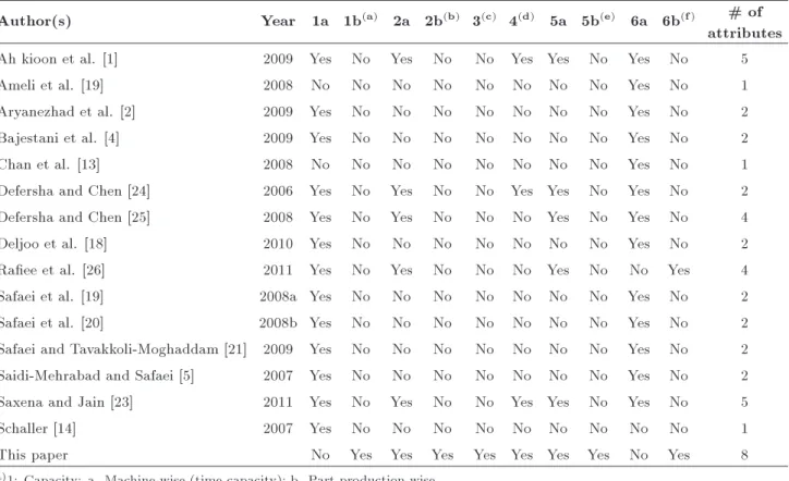
Table 1 addresses the distribution of some special attributes in cell formation papers which have focused on modeling techniques, as this paper, more than on solving methods. These studies have also another similarity with this paper, which is they discuss mostly the number of machines needed in each cell and each period as well as the amount of purchasing and removing (selling) them.
3. Assumptions of the proposed mathematical model
1. Parts move in sub-lots in dierent routes as as-sumed by Bajestani et al. [4] and in dierent periods to satisfy the same or other period's demand; 2. Back-orders are allowed. In other words, the index
t in decision variable xritt0 can be bigger than t0,
which means production can be done to satisfy an earlier requested demand that leads to backorder cost. In this case, the production lots are not
Table 1. Comparison between this paper and the ones in the literature regarding their attributes. Author(s) Year 1a 1b(a) 2a 2b(b) 3(c) 4(d) 5a 5b(e) 6a 6b(f) # of
attributes
Ah kioon et al. [1] 2009 Yes No Yes No No Yes Yes No Yes No 5
Ameli et al. [19] 2008 No No No No No No No No Yes No 1
Aryanezhad et al. [2] 2009 Yes No No No No No No No Yes No 2
Bajestani et al. [4] 2009 Yes No No No No No No No Yes No 2
Chan et al. [13] 2008 No No No No No No No No Yes No 1
Defersha and Chen [24] 2006 Yes No Yes No No Yes Yes No Yes No 2
Defersha and Chen [25] 2008 Yes No Yes No No No Yes No Yes No 4
Deljoo et al. [18] 2010 Yes No No No No No No No Yes No 2
Raee et al. [26] 2011 Yes No Yes No No No Yes No No Yes 4
Safaei et al. [19] 2008a Yes No No No No No No No Yes No 2
Safaei et al. [20] 2008b Yes No No No No No No No Yes No 2
Safaei and Tavakkoli-Moghaddam [21] 2009 Yes No No No No No No No Yes No 2 Saidi-Mehrabad and Safaei [5] 2007 Yes No No No No No No No Yes No 2
Saxena and Jain [23] 2011 Yes No Yes No No Yes Yes No Yes No 5
Schaller [14] 2007 Yes No No No No No No No No No 1
This paper No Yes Yes Yes Yes Yes Yes Yes No Yes 8
(a)1: Capacity: a. Machine-wise (time capacity); b. Part production-wise. (b)2: Lot-splitting: a: Lot-aplitting among batches; b. Lot-splitting among time. (c)3: Machine depreciation.
(d)4: Machine maintenance cost.
(e)5: Sub-contracting: a. Sub-contracting cost; b. Sub-contracting as a production route. (f)6: Inter-cell movement: a. constant; b. based on distance.
assigned any holding cost and immediately charged to their related demand;
3. Sub-contracting is allowed and for the ease of modeling, we consider the sub-contracting of part i as the last route of part i indexed by Ri. Therefore,
no set-up cost would be assigned to route number Ri;
4. Demand of each part is known and deterministic. This assumption is found well in literature; 5. The operation cost and processing time of each part
getting processed on any machine are considered constant and independent of lot sizes; therefore, they are not considered in the problem;
6. Set-up time is considered for machines and, accord-ing to the types of parts decided to be produced in a period (lucky types), the relating machines have to be set up in the beginning of that period; 7. Intra-cell movement costs dened per unit are
con-stant for each part and independent of the distance between machines in a cell;
8. Inter-cell movement costs are constant for each part but dened per unit and per distance. That means they should be multiplied by the distance between the two cells. A From-To distance matrix is dened as LL= fall0g where all0 is the distance between
cell l and cell l0;
9. Machines can be added (purchased) or removed (sold) to or from each cell in each period. In the case of selling machine, their depreciation can be considered in an n-period planning horizon as a positive statement of costs or an income of money. If Nkl(t) shows the number of machines from type k
in cell number l during period t, then, according to this assumption,PNkl(t) PNkl(t 1) can have
either positive or negative sign or can be zero. In the positive case, we will assign a procurement or machine cost because it means we have to purchase machines, and in the negative case, we will assign a xed income (a negative statement of costs), which reects the meaning of the book-values of the machines sold. For the sake of easiness, the
method of depreciation used is the Straight Line (SL) method. At the end of the planning periods, all of the machines are sold. The useful life of the machines is bigger than the planning horizons; 10. In addition to lot-splitting among routes, such as
that considered by Defersha and Chen [24], lot-splitting can also be considered among time periods by taking into account the demand information of the parts. For example, if we need 200 units of product X in period 10, the holding costs could imply that it would be more economical to produce 90 units in period 5, 80 units in period 7, and 30 units in period 9 to satisfy the demand of period 10 instead of producing all the 200 units in period 10; 11. Part Production Capacity (PPC) is dened which reects the fact that a company might not be able to deal with more than a specic number of part types in each period;
12. The maximum and minimum numbers of machines of each type in each cell are dened in order to avoid disturbance of system when removing or adding machines. These bounds remain constant over periods. This assumption has been used well in literature (e.g. [25]);
13. Each type of machine might process dierent parts in dierent periods (machine exibility). This as-sumption has been extracted from Aryanezhad et al. [2];
14. Machines have procurement cost during their pres-ence in the system; therefore, procurement cost is charged;
15. Production waste is considered. The additional (if exists) dierence between the production sub-lot sizes for a specic period and that period's demand is called waste and is attempted to be minimized. Notations and sets
T Number of planning periods indexed by t or t0 or t00
I Number of part types indexed by i Ji Number of operations of part i indexed
by j
Ri Number of routes of part i indexed by
r
Fri Set of machines available in route r of
part i
K Number of machine types indexed by k L Number of cells indexed by l or l0
uk Number of depreciation periods (useful
life) of machine type k, which is bigger than T
Parameters
P Mk Machine type k's purchasing cost
(which is simply equal to BVk0)
BVk(t0; t) Book value of machine type k
purchased in period t0 planned to be
soldin period t
SVk Salvage value of machine type k
Dk Depreciation value of machine type k
obtained from SL method
Mak Maintenance cost of machine type k
per period
BigM Large positive number Sk Set-up cost of machine k
Pi(t) Production cost of part i in period t
hi Holding cost of part i per period
bi Back-order cost of part i per period
Wi Production waste cost of part i per
unit of production
i Sub-contracting cost of part i per unit
of production
P C(t) Production capacity of period t MC(t) The maximum number of part types
that can be produced in period t LBMl Lower bound of the number of
machines in cell l
UBMl Upper bound of the number of
machines in cell l
di(t) Demand of part i in period t
i Inter-cell movement cost of part i per
unit per distance
i Intra-cell movement cost of part i per
unit (regardless of distance)
LL= fall0g From-to distance matrix of cells; all0
is the distance between cell l and l0
(intra-cell distance) Decision variables
Integers:
BMk(t0) Number of machines type k purchased
in the beginning of period t0
SMk(t; t00) Number of machines type k purchased
in the beginning of period t0 and sold
in the beginning of period t00
Nkl(t) Number of machines type k available
in cell l for period t
xri(t; t0) Sub-lot size of part i processed in route
r in period t in order to satisfy period t0s demand
Binary: qi(t) =
8 > < > :
1 if part i allowed to be produced in period t
0 o.w. wri(t) =
8 > < > :
1 if router r is set up for part i in period t
0 o.w. jirl(t) =
8 > < > :
1 if operation j in router of part i is processed in cell during period t 0 o.w.
rkl(t) =
8 > < > :
1 if machine k is assigned to cell 1 in period t
0 o.w. Mathematical model
Minimize Z =XK
k=1
Mak
XT t0=1
T
X
t00=t0+1
(t00
t0):SM k(t0; t00)
+XI
i=1 T
X
t0=1
Wi XT t=1 Ri X r=1
Xri(t; t0) di(t0)
+XRi
r=1 I X i=1 T X t=1 T X
t0=1
himaxf0; t0 tg
+ bimaxf0; t t0g
xri(t; t0)
+
RXi 1
r=1 I X i=1 T X t=1 T X
t0=1
Pi(t):Xri(t; t0) T
X
t0=1
T 1X t00=t0+1
BVk(t0; t00):SMk(t0; t00) T
X
t0=1
BVk(t0; T ):Nk1(T )
+XT
t0=1
P Mk:BMk(t0)
+ I X i=1 T X t=1
qi(t) RXi 1
r=1
wri(t)
X
k2Fri
Sk
!!
+XI
i=1 T X t=1 T X
t0=1
i:XRii(t; t0)
+12XI
i=1 RXi 1
r=1 JXi 1
j=1 T X t=1 T X
t0=1
L
X
l=1
j+1;ril(t)
jril(t)iXri(t; t0)
+12
I
X
i=1 RXi 1
r=1 JXi 1
j=1 T X t=1 T X
t0=1
L
X
l=1 L
X
l0=1
j+1;ril0(t)jril(t)iall0Xri(t; t0); (1)
L
X
l=1
jril(t) = wri(t) 8j; r; i; t; (2) L
X
l=1
Nkl(t00) L
X
l=1
Nkl(t00 1) = BMkt00 SMkt0t00
8k; t0; t00
where t0< t00; (3)
LBMl L
X
l=1
Nkl(t) UBMl 8k; l; t; (4)
rkl(t) Nkl(t) 8k; l; t; (5)
Nkl(t) BigM:rkl(t) 8k; l; t; (6)
Dk = (P Mk SVk)=uk 8k; (7)
BVk(t0+1)t00+ Dk= BVkt0t00 8k; t00; (8)
I
X
i=1
qit MCt 8t; (9)
RXi 1
r=1
Xri(t; t0) BigM:qit 8i; t; t0; (10) T X t=1 Ri X r=1
Xri(t; t0) di(t0) 8i; t0; (11)
Ii(t0 1)+ T X t=1 Ri X r=1
Xri(t; t0)=di(t0) + Ii(t0) 8i; t0;
(12)
T
X
t0=1
RXi 1
r=1 I
X
i=1
Eq. (1) shows the objective function. In the second statement, the production waste is attempted to be minimized. The benet of using this statement in the objective function is that it forces the surplus of Relation (11) to be zero instead of dening it as a hard constraint (LHS = RHS) in the rst place. Relation (11) implies that the sum of production sub-lot sizes which are indented to satisfy period t0s demand
have to be at least equal to it. Eventually, the second statement of objective function and Relation (11) tries to satisfy demand and minimize production waste on the other hand. Also, Relation (11) reects another consideration that in order to satisfy a specic period's demand, we are allowed to produce in all the planning periods. For example, the satised demand of period 5 of a CFP with 8 planning horizons can consist of sub-lots produced in periods 1, 6, and 8. On the other hand, it means that back-order is allowed. Relation (13) mainly aects this decision since it allows only a maximum production volume in each period. The sub-lots produced before the period they are intended to satisfy its demand charge holding cost to the system until that specic period, and the sub-lots produced after the period they are intended to satisfy its demand charge back-order cost regarding the number of periods they have delayed in production; but, they do not charge any holding cost since they would be immediately fed into the related demand. These holding and back-order costs are implied in the third statement of objective function. Also, note that Eq. (12) is the inventory balance equation. The fourth statement of the objective function implies the production cost of sub-lot sizes.
The next three statements (fth to seventh) and the rst statement of objective function are related to the fact that we are allowed to purchase and sell machines from any type. The fourth statement charges the procurement cost of the machines due to their presence duration in the system. The fth statement utilizes the denition of decision variable SM (number of sold machines) and parameter BV (book-value or the income achieved from selling a machine) to calculate the income received from selling machines according to their book-value in the specic period they are sold. Notice that the second summation in this statement is up to T 1; thus, it does not interrupt the sixth statement. Also, the second summation in the rst and fth statements begins at t00= t0+ 1 to automatically
imply that obviously a machine is sold at least a period after it was purchased. As mentioned in the assumptions, the sixth statement calculates the income from selling all of the machines remaining in the end of the planning horizons regarding their book-value. The seventh statement calculates the purchasing cost of all the purchased machines. The depreciation method used in this paper's problem is the Straight Line (SL)
method, which calculates the value of depreciation that decreases the book-value of the machine in Eq. (7) and calculates the book-value for every period of all machine types in Eq. (8). Eventually, Eq. (3) simply implies that the dierence between the numbers of machines of two subsequent periods is equal to the dierence between the numbers of machines purchased and sold. This equation is used to calculate Nkl(t).
Also, since the LHS is related to the number of machines in cells while the RHS is the number of sold and purchased machines regardless of what happens in cells, by LHS(3) = RHS(3), the concepts of selling and purchasing machines are attached to the number of machines in cells and, therefore, they would not be independent of the CFP situation. Also, notice that removing the machines may cause disturbance in the cellular manufacturing system if all of the units available from machine type k might be sold and, therefore, it would not be possible to produce a specic part type which needs to be operated at least once on a machine type k. Therefore, a lower bound and an upper bound are dened for the number of machines of each type in each cell in order to avoid this disturbance. This approach has been used well in literature, e.g. in the works done by Defersha and Chen [24]. Relation (4) explains this constraint.
As mentioned in the assumptions, the PPC con-straint allows the system to produce only at most a specic number of various part types in a period as Relation (9) implies. Binary variable q is dened to show which part types are allowed (which makes them lucky) and which ones are not allowed to be produced in a period, although an unlucky part can still be sub-contracted if necessary. Therefore, Relation (10) avoids the production of a part type in a period which is decided not to be one of the lucky part types. Now, according to the denition of routes for each part type, any lucky part type in a specic period needs a number of machine types to be operated on. These machine types related to a route r are gathered in a set named Fri. For example, if route number
3 for part type 4 is to be processed respectively on machine types 4, 1, 2, 4, and 3 (4 ! 1 ! 2 ! 4 ! 3), then simply F34 = f1; 2; 3; 4g. Therefore, these
machines need be set up at the beginning of period to be ready for operating the lucky part type. Binary variables q and w (reecting the number of routes decided to be assigned to the lucky part type in that period) gather together to calculate the whole periods' machine set-up cost in the eighth statement of objective function. Note that the set-up cost's route summation is up to Ri 1. That is because, as considered, the
last number of the route index (Ri) is assigned to
sub-contacting. This consideration is mainly used in order to eliminate an additional statement for sub-contacting in the inventory balance constraint. The
ninth statement of the objective function calculates the cost of lots contracted. Notice that even sub-contracted sub-lots are allowed to be back-ordered since the route summation of Relation (11) is up to Ri.
And the last but not least signicant two state-ments of objective function calculate the inter-cell and intra-cell movement costs, respectively. These statements have been extracted from the objective function of the model used by Raee et al. [26]. As considered, the intra-cell movement cost is distance-dependent and is multiplied by the distance between cells instead of its unit cost. Eq. (2) is extracted from Defersha and Chen [25] to imply that an operation is allowed to be assigned only once to a part type in a route and specic period.
4. The proposed ant colony optimization algorithm
According to the fact that CFP is an NP-hard combi-natorial optimization problem, exact methods cannot be always usable. In other words, the complexity of the CFP forces us to use heuristics and meta-heuristics to deal with its large-size problems. In this paper, Ant Colony Optimization (ACO) has been proposed to solve large-size problems of this kind. Many nu-merical experiments have been conducted so far for combinatorial problems. For example, Dorigo et al. [27] compared ACO, Genetic Algorithm (GA), Evolution-ary Programming (EP), Simulated Annealing (SA), and hybrid GA-SA for some combinatorial samples and concluded that ACO outperformed other tested algorithms. On the other hand, there are instances of ant-based algorithms in cell formation literature such as Megala and Rajendran [28], and Farahani and Ho-seini [29]. Both mentioned papers reported application of ant-based algorithms to CFP using clustering-based approaches. In both ones, the authors utilized 0-1 matrix elements to indicate whether a specic part needed to meet a specic machine.
To structure ACO algorithm and its numerous versions, Dorigo and his colleagues were inspired by the nature of ants in nding their paths from the nest to the food. Ants use a material called pheromone to com-municate with each other along their course. Dorigo et al. [27] proposed the rst ant-based algorithm and, afterwards, some versions were presented by Stutzle and Dorigo [30] to solve the well-known Quadratic Assignment Problem (QAP). Their proposed versions included Ant System (AS), Ant Colony System (ACS), ANTS-QAP, Min-Max AS, Fast ANT (FANT), and Hybrid Ant System-QAP (HAS-QAP). Since ACO is a well-established meta-heuristic, its introduction will be skipped here and the readers are referred to [31,32] for comprehensive description of ACO and its numerous applications. The pseudo-code of the proposed ACO
Figure 1. Pseudo-code of the proposed ACO.
in this paper can be seen in Figure 1. The next two sections describe more details about the proposed ACO algorithm in this paper.
4.1. Solution representation
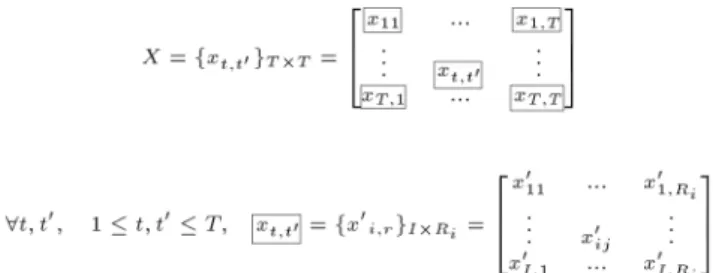
The solution representation is performed by two ma-trices, a dimensional normal matrix and a two-dimensional super matrix as shown in Figures 2 and 3, respectively.
In Figure 2, srij is a binary variable, 1 if machine
type i is allocated to cell number j and 0 otherwise. In Figure 3, X is a super matrix, that is, every element of it, described as xt;t0, is a matrix itself. This super
matrix contains the production plan. In other words, it contains all the variables of xritt0 described in the
mathematical model. Actually, X is a Ri I T T
matrix and it has turned into a super matrix for the ease of modeling and ignoring dimension complexities. As can be seen in the pseudo-code in Figure 1,
Figure 2. Solution representation corresponding to the machine-cell allocation.
Figure 3. Solution representation corresponding to the production plan.
the ACO algorithm here rst evaluates SR(t), which
means it species the machine-cell allocation, and then evaluates the production plan.
4.2. Attractiveness calculation
As can also be seen in the pseudo-code, to complete the current solution by the articial ant of the algorithm, rst, it is decided whether the machine is allocated to the cell. To do so, attractiveness of any possible candidate is calculated using Eq. (14):
mc= 1
1 +PCc=1Z1mc+ Z2mc: (14)
Attractiveness is calculated for feasible candidates, i.e. the cells of which the maximum sizes are not violated. 5. Numerical results
In this section, three numerical examples will be solved to validate the model. Regarding the size of the main data sets, these three examples are categorized into small, medium, and large-size problems. The rst two categories are solved by both exact method, Branch And Reduce Optimization Navigator (BARON) by using General Algebraic Modeling System (GAMS) software, and meta-heuristic method, the proposed ACO algorithm in Section 4. The results of these two methods are compared and, then, the ACO algorithm is utilized to solve the large-size problem. The pa-rameter data of all the test problems are categorized into four groups of machine, production, cost, and cellular-related data. The solution data have also been categorized into two groups of machine-cell allocation plan and production plan.
5.1. Small-size test problem
The small-size test problem considered here is a 2-period dynamic cell formation with 4 parts, which have at most 3 routes and each route has at most 3 operations; 4 machine types are needed and there are 2 cells planned. Although it is considered that not all the parts can be sub-contracted, the value of Ri for
each i will be considered as the number of production routes of part i plus one, even if that part does not have the possibility to be sub-contracted. This is to avoid the confusion of model when it encounters the sub-contracting statements of the objective function for parts with no sub-contraction and will be considered in all test problems. However, in this test problem, sub-contracting is allowed for all part types.
The parameter data for the test problem pre-sented here are categorized into four groups of machine, production, cost, and cellular-related. Tables 2 to 6 show these data, respectively. As explained in Section 2, the machine-related parameters in Table 2 have been set in a way that the depreciation values are bigger than
Table 2. Machine-related parameters of the small-size problem.
Machine
types P M SV N D Ma Setup
1 113 41 6 12.00 11.5 6
2 124 51 7 10.43 8.5 8
3 88 48 4 10.00 9 8
4 130 55 8 9.38 9.5 9
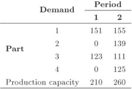
Table 3. Production-related parameters of the small-size problem; part type demand.
Demand Period
1 2
Part
1 151 155
2 0 139
3 123 111
4 0 125
Production capacity 210 260
Table 4. Production-related parameters of the small-size problem; part type routes and operations.
Operation Machine type
order 1 2 3 4
Part
1 1 2 1
2 1 1 2 3
2 1 2 3
3 1 1 2 3
4 1 3 1 2
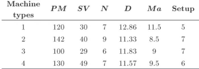
maintenance cost (and even setup costs); therefore, the case would be realistic. For instance, the depreciation value of machine type one will be (113 41)=6 = 12 per period, which is bigger than 11.5; or depreciation value of machine type 2 is:
DM2= 124 517 = 10:43 > MaM2 = 8:5:
The demand values in Table 3 show the signicance of lot-splitting in this numerical example because, as can be seen, the sum of demands exceeds the production capacity dened for that period. The holding cost values in Table 5 also refer to this point. Table 4 clearly explains the part production routes on dierent machine types. For instance, part type 2 can be manufactured in two ways. It can be processed by either machine types 1, 3, and 2, respectively, or machine types 1, 4, and 3, respectively. The from-to matrix in Table 6 is assumed symmetric.
The exact and meta-heuristic methods solved the model on an Intel® Core i5-520M processor 2.40 GHz
Table 5. Cost-related parameters of the small-size problem.
Holding Back-order Intercellular Intracellular Sub-contract
Production in period
Waste
1 2
Part
1 0.51 0.02 0.70 0.12 0.16 0.20 1.00 0.05
2 1.05 0.01 0.80 0.13 0.24 0.30 0.70 0.05
3 0.77 0.03 0.80 0.12 0.24 0.25 0.05 0.1
4 0.75 0.01 0.90 0.12 0.16 0.20 0.50 0.005
solution data were identical. The optimal production plan shown in Table 6 generated by the model is logical according to the tough capacity constraints. Also, optimal allocations of machines, and procurement and sales plans are shown in Tables 7 and 8. These tables
Table 6. Cellular-related parameters of the small-size problem; cellular from-to distance matrix.
From/to C1 C2
C1 0 1.5
C2 1.5 0
Table 7. Solution data of the small-size problem; production plan.
Part Route
Produced in period (*) to satisfy demand
of period (#)
#1 #2
1 2 1 2
1 1 100 6 49 50
2 45 56
2
1 16
2 32
3 60 24
3 1 61 50 38
2 12 35 38
4 1 68
2 57
are absolutely related to the needs of the optimal production plan.
The lucky parts of periods 1 and 2 were f1; 3g and f1; 2; 3; 4g, respectively. All of the demands (total demand = Pdi(t) = 804) are exactly satised and
summing up the production volume of the system concludes that the system has used up its production capacity, which is PP C = 210 + 260 = 470. The remaining demands (334 = Pdi(t) PP C) were
satised by sub-contraction. 5.2. Medium-size test problem
The medium-size problem considered here includes 3 periods and 5 part types, each having at most 4 routes, where again the last route is specied for sub-contracting and we may logically say the part types having the least routes available for production are more likely to be sub-contracted. Each production route has at most 3 operations. There are 4 machine types and 3 cells needed. In this test problem, only part types 1 and 4 are allowed to be sub-contracted. The categorized parameter data of the test problem are shown in Tables 9 to 13.
Table 9. Machine-related parameters of the medium-size problem.
Machine
types P M SV N D Ma Setup
1 120 30 7 12.86 11.5 5
2 142 40 9 11.33 8.5 7
3 100 29 6 11.83 9 7
4 130 49 7 11.57 9.5 6
Table 8. Solution data of the small-size problem; machine allocation and procurement and sales plan.
Period 1 Period 2
Machine
BMk(1) SMk(1; t00) Nkl(1) Machine BMk(2) SMk(2; t00) Nkl(2)
type 2 Cell 1 Cell 2 type 2 Cell 1 Cell 2
1 0 0 0 0 1 2 1 1
2 2 0 1 1 2 3 2 3
3 2 0 1 1 3 4 3 3
Table 10. Production-related parameters of the medium-size problem; part type demand.
Demand Period
1 2 3
Part
1 151 155 240
2 0 139 210
3 123 111 102
4 0 125 190
5 111 140 100
Production capacity 576 426 561 Table 11. Production-related parameters of the medium-size problem; part type routes and operations.
Operation Machine type
order 1 2 3 4
Parts
1 1 2 1
2 1 1 3 2
2 1 3 2
3 1 1 2 3
2 1 2
4 1 3 1 2
5
1 2 1
2 2 1 3
3 2 1
The exact and meta-heuristic methods solved the model on an Intel® Core i5-520M processor 2.40 GHz
CPU in 6 minutes and 17.067 seconds, and 20.357 seconds, respectively, and their solution data were identical. Tables 14 and 15 represent the solution data of this rather more complex test problem than the previous one.
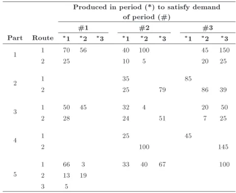
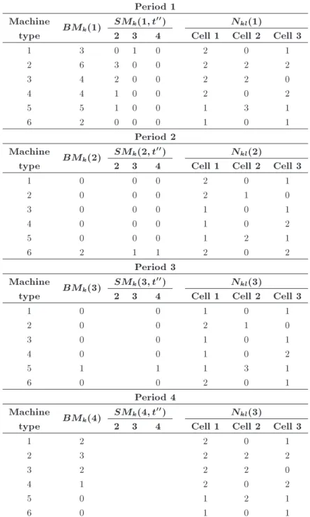
The lucky parts of periods 1, 2, and 3 were f1; 2; 3; 4; 5g, f1; 3; 5g, and f1; 2; 3; 5g, respectively.
Table 13. Cellular-related parameters of the medium-size problem; cellular from-to distance matrix.
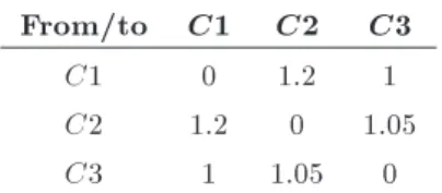
From/to C1 C2 C3
C1 0 1.2 1
C2 1.2 0 1.05
C3 1 1.05 0
The optimal production plan here again shows exact satisfaction of demands with combination of produc-tion sub-lot sizing and sub-contracting. Although, summing up the production volume reveals that the system has not used up its capacity in almost all of the periods. In fact, the production capacity (PP C = 1563) diers slightly from the real production volume (PTt0=1
PT
t=1
PI
i=1
PRi 1
r=1 Xritt0 = 1562).
5.3. Large-size test problem
The large-size problem considered here includes 4 periods and 8 part types, each having a dierent number of routes. Sub-contracting has been considered for all parts, even the ones having many production routes available. There are 6 machine types and 3 cells planned. The categorized parameter data of the test problem are shown in Tables 16 to 20.
As shown in Table 16, again, none of the main-tenance and setup costs exceed the depreciation values to keep the problem in a realistic manner. This time, one of the machine types has salvage value of zero; which means it will be completely obsolete at the end of its useful life. As can be seen in Table 17, there are a variety of demands/periods for part types. Also, demands for a few part types in some periods are zero, which means the model may have the chance to choose the lucky parts. Table 18 shows that each production route has at most 3 operations. The required orders of these operations for manufacturing the part type have also been described. The competition between the sub-contraction and production costs in Table 19 is interesting. In some cases, one is bigger than the other and in some cases, they have a slight dierence. Each of these cases aects the optimality of problem dierently.
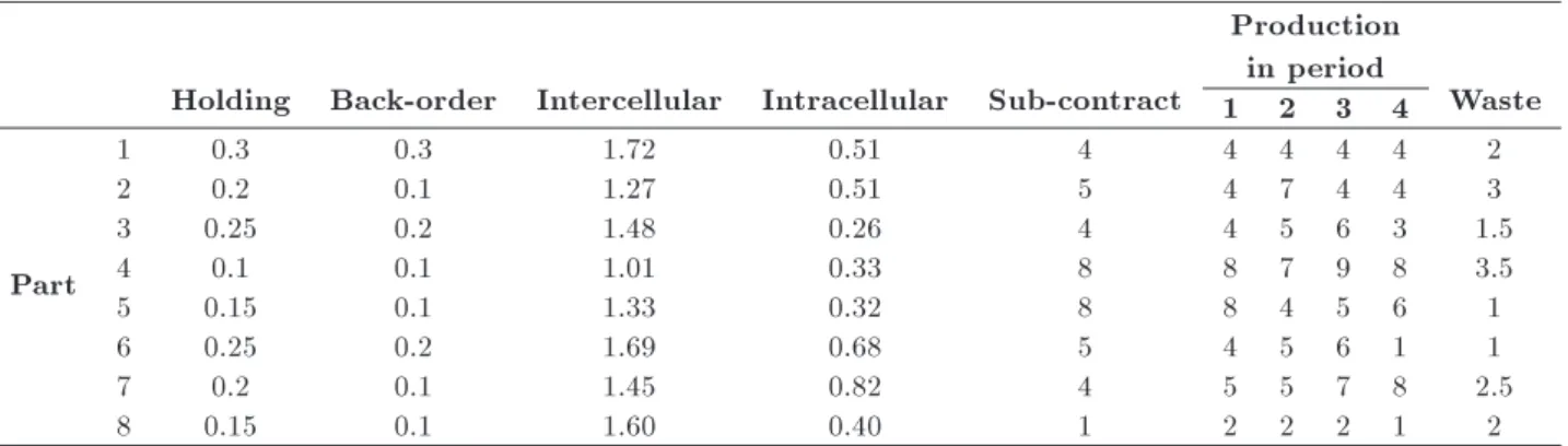
Table 12. Cost-related parameters of the medium-size problem.
Hold Back Intercellular Intracellular Sub-contract
Production in period
Waste
1 2 3
Part
1 0.3 0.02 0.70 0.12 0.16 0.02 1.00 1.00 0.05
2 0.2 0.01 0.80 0.13 0.24 0.40 0.70 0.80 0.05
3 0.25 0.03 0.80 0.12 0.24 0.05 1.05 1.90 0.1
4 0.1 0.01 0.90 0.12 0.16 1.00 1.50 1.70 0.005
Table 14. Solution data of the medium-size problem; production plan.
Part Route
Produced in period (*) to satisfy demand of period (#)
#1 #2 #3
1 2 3 1 2 3 1 2 3
1 1 70 56 40 100 45 150
2 25 10 5 20 25
2 1 35 85
2 25 79 86 39
3 1 50 45 32 4 20 50
2 28 24 51 7 25
4 1 25 45
2 100 145
5
1 66 3 33 40 67 100
2 13 19
3 5
Table 15. Solution data of the medium-size problem; machine allocation and procurement and sales plan. Period 1
Machine BMk(1) SMk(1; t00) Nkl(1)
type 2 3 Cell 1 Cell 2 Cell 3
1 4 1 1 2 0 2
2 7 2 1 2 3 2
3 6 3 0 2 2 2
4 6 1 1 1 3 2
Period 2
Machine BMk(2) SMk(2; t00) Nkl(2)
type 2 3 Cell 1 Cell 2 Cell 3
1 0 0 2 0 1
2 0 0 1 3 0
3 0 0 1 1 1
4 0 0 1 2 2
Period 3
Machine BMk(3) SMk(3; t00) Nkl(3)
type 2 3 Cell 1 Cell 2 Cell 3
1 0 1 0 1
2 0 1 2 0
3 0 1 1 1
4 0 1 1 2
The proposed ACO algorithm solved the large-size test problem in 1 minute and 32.764 seconds on the same computer utilized for the previous test problems. Tables 21 and 22 show solution data of this test problem.
The model decided to choose the part types f1; 3; 4; 6; 8g, f1; 3; 5; 7g, f1; 2; 3; 8g, and f1; 4; 5; 7g, respectively, for periods 1, 2, 3, and 4 as the lucky parts. This time, the whole production capacity was used up and near 66% of the demands were satised
Table 16. Machine-related parameters of the large-size problem.
Machine
types P M SV N D Ma Setup
1 1000 50 7 135.71 100 10
2 800 0 6 133.33 111 12
3 1050 100 7 135.71 105 11 4 1100 100 7 142.86 101 11
5 2000 200 10 180.00 89 9
6 1400 250 9 127.78 96 10
Table 17. Production-related parameters of the large-size problem; part type demand.
Demand Period
1 2 3 4
Part
1 102 105 177 103
2 80 0 150 0
3 95 86 113 138
4 44 0 53 70
5 0 65 65 46
6 71 18 0 24
7 0 41 32 17
8 40 42 0 50
Production capacity 371 281 407 141
by the total production volume. The other 34% were consigned to sub-contraction. Table 22 shows the variety of machines bought and sold in dierent periods. In fact, this variety can be seen more clearly in Table 23, which shows the number of machines required in each period. This number decreases through 2 periods and, then, suddenly increases to a value near its initial one. This trend can also be somehow tracked in the production plan and the needs of production routes to satisfy back-ordered or up-coming demands.
6. Conclusions and future research
In this paper, a mathematical model including some new and special concepts was proposed combining pro-duction planning with engineering economics. Main-tenance cost was considered for the machines bought and evaluated according to the time they were decided to be sold. Lot sizes of part types were considered, which means they were assumed as physical units having costs, especially inter and intra-cell move-ment costs. The combination of production, sub-contracting, back-order, and holding costs led to some numerical results, in which, in some cases, the model
Table 18. Production-related parameters of the large-size problem; part type routes and operations.
Operation Machine type
order 1 2 3 4 5 6
Part
1 1 2 1 3
2 3 2 1
2
1 1 2
2 1 2 3
3 1 2
3 1 2 1
2 1 2 3
4
1 1 3 2
2 1 2 3
3 2 1 3
4 2 1
5 1 3 2 1
6 1 1 2
2 2 1
7 1 1 3 2
2 1 2
8 1 1 2 3
2 1 2 3
decided that it would be better to back-log some orders or leave the rest of the production up to sub-contracting. Three categories of test problems (small, medium, and large) were solved by both exact and a meta-heuristic algorithms. A meta-heuristic algorithm based on ACO was proposed to cope with the large-size samples of the proposed mathematical model.
As future research directions, according to the fact that the concept of selling machines leads to negative cost function or, in other words, prot, it is recommended that other concepts of engineering economics also be embedded in this problem in order to craft a more accurate solution. For example, market values of machines, which are not necessarily equal to the book-values (leading to capital gain or capital loss concepts), can be considered with impreciseness in the parameters; simple replacement analysis can be done according to the marginal cost approach. Also, nite useful life of machines can cause problems since some of them can turn obsolete before the job is
Table 19. Cost-related parameters of the large-size problem.
Holding Back-order Intercellular Intracellular Sub-contract
Production in period
Waste
1 2 3 4
Part
1 0.3 0.3 1.72 0.51 4 4 4 4 4 2
2 0.2 0.1 1.27 0.51 5 4 7 4 4 3
3 0.25 0.2 1.48 0.26 4 4 5 6 3 1.5
4 0.1 0.1 1.01 0.33 8 8 7 9 8 3.5
5 0.15 0.1 1.33 0.32 8 8 4 5 6 1
6 0.25 0.2 1.69 0.68 5 4 5 6 1 1
7 0.2 0.1 1.45 0.82 4 5 5 7 8 2.5
8 0.15 0.1 1.60 0.40 1 2 2 2 1 2
Table 20. Cellular-related parameters of the large-size problem; cellular from-to distance matrix.
From/to C1 C2 C3
C1 0 2.13 2.3
C2 2.13 0 1.97
C3 2.3 1.97 0
done. These kinds of assumptions can be very useful in providing a comprehensive decision making model for managers. Furthermore, other concepts like taxation, operation time, reliability, and reconguration cost can also be considered simultaneously with depreciating machines.
Table 21. Solution data of the large-size problem; production plan. Produced in period (*) to satisfy demand of period (#)
Part Route #1 #2 #3 #4
1 2 3 4 1 2 3 4 1 2 3 4 1 2 3 4
1 12 2010 5 55 2040 10 10 3 407 3010 15 55 10 3015 2525 55
3 50 7 10 5 5 2 40 25 3 5
2
1 50
2 5 100
3 25
4 50
3 12 355 15 10 9 10 2525 16 20 1520 1018 20 2015
3 10 10 7 10 17 15 10 30 15 10
4
1 15 25 5
2 20 4 20
3 5 4 5 30
4 10 4 5 5
5 4 6
5 1 60 10 18
2 5 5 60 18
6 12 71
3 18 24
7 12 1515 88 2
3 8 3 20 17
8 12 12
Table 22. Solution data of the large-size problem; machine allocation and procurement and sales plan. Period 1
Machine BMk(1) SMk(1; t00) Nkl(1)
type 2 3 4 Cell 1 Cell 2 Cell 3
1 3 0 1 0 2 0 1
2 6 3 0 0 2 2 2
3 4 2 0 0 2 2 0
4 4 1 0 0 2 0 2
5 5 1 0 0 1 3 1
6 2 0 0 0 1 0 1
Period 2
Machine BMk(2) SMk(2; t00) Nkl(2)
type 2 3 4 Cell 1 Cell 2 Cell 3
1 0 0 0 2 0 1
2 0 0 0 2 1 0
3 0 0 0 1 0 1
4 0 0 0 1 0 2
5 0 0 0 1 2 1
6 2 1 1 2 0 2
Period 3
Machine BMk(3) SMk(3; t00) Nkl(3)
type 2 3 4 Cell 1 Cell 2 Cell 3
1 0 0 1 0 1
2 0 0 2 1 0
3 0 0 1 0 1
4 0 0 1 0 2
5 1 1 1 3 1
6 0 0 2 0 1
Period 4
Machine BMk(4) SMk(4; t00) Nkl(3)
type 2 3 4 Cell 1 Cell 2 Cell 3
1 2 2 0 1
2 3 2 2 2
3 2 2 2 0
4 1 2 0 2
5 0 1 2 1
6 0 1 0 1
Table 23. Solution data of the large-size problem; number of machines in each period.
PK k=1
PL
l=1Nkl(t)
Period
1 2 3 4
Total number of machines available 24 19 18 23
References
1. Ah kioon, S., Bulgak, A.A. and Bektas, T. \Integrated
cellular manufacturing systems design with production planning and dynamic system reconguration", EUR. J. OPER. RES., 192, pp. 414-428 (2009).
2. Aryanezhad, M.B., Deljoo, V. and Mirzapour
Al-e-hashem, S.M.J. \Dynamic cell formation and the worker assignment problem: a new model", Int. J. Adv. Manuf. Technol., 41, pp. 329-342 (2009).
3. Muruganandam, A., Prabhaharan, G., Asokan, P. and
Baskaran, V. \A memetic algorithm approach to the cell formation problem", Int. J. Adv. Manuf. Technol., 25, pp. 988-997 (2005).
4. Bajestani, M.A., Rabbani, M., Rahimi-Vahed, A.R.
and Baharian Khoshkhou, G. \A multi-objective scat-ter search for a dynamic cell formation problem", Com-puters & Operations Research, 36, pp. 777-794 (2009).
5. Saidi-Mehrabad, M. and Safaei, N. \A new model of dynamic cell formation by a neural approach", Int J. Adv. Manuf. Technol., 33, pp. 1001-1009 (2009).
6. Papaioannou, G. and Wilson, J.M. \ The evolution of
cell formation problem methodologies based on recent studies (1997-2008): Review and directions for future research", European Journal of Operational Research, 206, pp. 509-521 (2010).
7. Jolai, F., Tavakkloi-Moghaddam, R., Golmohammadi,
A. and Javadi, B. \An Electromagnetism-like algorithm for cell formation and layout problem", Expert Syst. Appl., 39(2), pp. 2172-2182 (2012).
8. Wei, N.C., Liao, T.J., Chao, I.M., Wu, P. and Chang,
Y.C. \An electromagnetism-like mechanism method for solving dynamic cell formation problems", Journal of Asian Scientic Research, 3(10), pp. 1022-1035 (2013).
9. Dalfard, V.M. \New mathematical model for problem
of dynamic cell formation based on number and average length of intra and intercellular movements", Applied Mathematical Modelling, 37(4), pp. 1884-1896 (2013).
10. Raei, H. and Ghodsi, R. \A bi-objective
mathematical model toward dynamic cell formation considering labor utilization", Applied Mathematical Modelling, 37(4), pp. 2308-2316 (2013).
11. Niakan, F., Baboli, A., Moyaux, T. and
Botta-Genoulaz, V. \A new multi-objective mathematical model for dynamic cell formation under demand and cost uncertainty considering social criteria", Applied Mathematical Modelling, 40(4), pp. 2674-2691 (2016).
12. Ariafar, S. and Ismail, N. \An improved algorithm
for layout design in cellular manufacturing systems", Journal of Manufacturing Systems, 28, pp. 132-139 (2009).
13. Chan, F.T.S., Lau, K.W., Chan, L.Y. and Lo,
V.H.Y. \Cell formation problem with consideration of both intracellular and intercellular movements", International Journal of Production Research, 46(10), pp. 2589-2620 (2008).
14. Schaller, J. \Designing and redesigning cellular
manufacturing systems to handle demand changes", Computers & Industrial Engineering, 53, pp. 478-490 (2007).
15. Liu, C.G., Yin, Y., Yasuda, K. and Lian, J. \A
heuristic algorithm for cell formation problems with consideration of multiple production factors", Int. J. Adv. Manuf. Technol., 46, pp. 1201-1213 (2010).
16. Pitombeira-Neto, A.R. and Goncalves-Filho, E.V.
\A simulation-based evolutionary multiobjective approach to manufacturing cell formation", Computers & Industrial Engineering, 59, pp. 64-74 (2010).
17. Javadian, N., Aghajani, A., Rezaeian, J. and Sebdani,
M.J.G. \A multi-objective integrated cellular manu-facturing systems design with dynamic system recon-guration", International Journal of Advanced Man-ufacturing Technology, 56(1-4), pp. 307-317 (2011).
18. Deljoo, V., Mirzapour Al-e-hashem, S.M.J., Deljoo,
F. and Aryanezhad M.B. \Using genetic algorithm to solve dynamic cell formation problem", Applied Mathematical Modelling, 34, pp. 1078-1092 (2010).
19. Safaei, N., Saidi-Mehrabad, M. and Jabal-Ameli,
M.S. \A hybrid simulated annealing for solving an extended model of dynamic cellular manufacturing system", European Journal of Operational Research, 185, pp. 563-592 (2008).
20. Safaei N., Saidi-Mehrabad, M.,
Tavakkoli-Mogha-ddam, R. and Sassani, F. \A fuzzy programming approach for a cell formation problem with dynamic and uncertain conditions", Fuzzy Sets and Systems, 159, pp. 215-236 (2008).
21. Safaei, N. and Tavakkoli-Moghaddam, R. \
Integrated multi-period cell formation and
subcontracting production planning in dynamic cellular manufacturing systems", Int. J. Production Economics, 120, pp. 301-314 (2009).
22. Wang, X., Tang, J. and Yung, K.l. \Optimization of
the multi-objective dynamic cell formation problem using a scatter search approach", Int. J. Adv. Manuf. Technol., 44, pp. 318-329 (2009).
23. Saxena, L.K. and Jain, P.K. \Dynamic cellular
man-ufacturing systems design: a comprehensive model", Int. J. Adv. Manuf. Technol., 53, pp. 11-34 (2011).
24. Defersha, F.M. and Chen, M. \A comprehensive
mathematical model for the design of cellular
manufacturing systems", Int. J. Production
Economics, 103, pp. 767-783 (2006).
25. Defersha, F.M. and Chen, M. \A linear programming
embedded genetic algorithm for an integrated cell formation and lot sizing considering product quality", European Journal of Operational Research, 187, pp. 46-69 (2008).
26. Raee, K., Rabbani, M., Raei, H. and Rahimi-Vahed,
A. \A new approach towards integrated cell formation and inventory lot sizing in an unreliable cellular
manufacturing system", Applied Mathematical
Modeling, 35(4), pp. 1810-1819 (2011).
27. Dorigo, M., Colorni, A. and Maniezzo, V. \An
investigation of some properties of an ant algorithm", In PPSN, 92, pp. 509-520 (1992).
28. Megala, N. and Rajendran, C. \An improved
ant-colony algorithm for the grouping of machine-cells and part-families in cellular manufacturing systems", International Journal of Operational Research, 17(3), pp. 345-373 (2013).
29. Hosseinabadi Farahani, M. and Hosseini, L. \An ant
colony optimization approach for the machine-part cell formation problem", International Journal of Compu-tational Intelligence Systems, 4(4), pp. 486-496 (2011).
30. Stutzle, T. and Dorigo, M., Ant Colony Algorithms
for Quadratic Assignment Problem: New Ideas in Optimization, McGraw Hill, New York (1999)
31. Dorigo, M. and Stutzle, T., Ant Colony Optimization,
32. Maniezzo, V., Gambardella, L.M. and De Luigi, F., Ant Colony Optimization: New Optimization Techniques in Engineering, Springer-Verlag (2004). Biographies
Masoud Rabbani is a Professor of Industrial En-gineering in the School of Industrial and Systems Engineering at University of Tehran. He has pub-lished more than 60 papers in international journals, such as European Journal of Operational Research, International Journal of Production Research, and International Journal of Production Economics, among others. His research interests include production-planning, design of inventory management systems, applied graph theory in industrial planning, and pro-ductivity management.
Sina Keyhanian is currently a PhD student of Industrial Engineering under a joint Ubbo Emmius Scholarship at University of Groningen and Amirk-abir University of Technology. He received his MS degree of Industrial Engineering from the Faculty of Engineering, University of Tehran, Iran, in 2012, where he also received his BS in 2010. He is the founder and former head of the University of Tehran's Iranian Mathematical Society for Engineers (UTIMSE-2009). He has also been teaching Calculus, Elementary and Advanced Engineering Economics, and Finance to undergraduate and graduate students since 2007.
His main scientic interests are pure and applied mathematics, game theory, analytic number theory, combinatory, articial intelligence, operations research, mathematical modelling and simulation, nance, and engineering economics.
Neda Manavizadeh accomplished her MSc in In-dustrial Engineering in the College of Engineering, University of Tehran, in 2005. She obtained her PhD in Industrial Engineering from the College of Engineering, University of Tehran. Currently, she is an Assistant Professor in the Industrial Engineering Department, KHATAM University, Tehran, Iran. Her research interests are production planning, supply chain man-agement, operations manman-agement, and Operations Re-search (OR).
Hamed Farrokhi-Asl received his BSc in Industrial Engineering from Khaje-Nasir University of Technol-ogy, Iran, in 2013. He continued his MSc studies at University of Tehran and graduated in 2014. He could publish 8 conference and journal papers based upon his Master's research at University of Tehran. He joined professor Rabbani's research team, who is a Professor in the school of Industrial Engineering at University of Tehran, as a Research Assistant. He initially started working on a new nature-inspired algorithm at Computer Laboratory of Iran University of Science & Technology. His interests include waste management, green supply chain, and optimization algorithms.