Sharif University of Technology
Scientia IranicaTransactions A: Civil Engineering www.scientiairanica.com
Estimation of scour downstream of a ski-jump bucket
using the multivariate adaptive regression splines
A.H. Haghiabi
Department of Water Engineering, Lorestan University, Khorramabad, Iran.
Received 11 August 2015; received in revised form 10 April 2016; accepted 22 August 2016
KEYWORDS Energy dissipation; Soft computing; Hydraulic structure; Scour depth; Spillways.
Abstract. In this paper, modeling the scour downstream of a ip bucket of spillways was considered using empirical formulas, soft computing techniques such as multilayer perceptron (MLP) neural network, and Multivariate Adaptive Regression Splines (MARS). For this purpose, 95 data sets were collected with regard to the most aective parameters on the scouring phenomena at downstream of spillways. During the MLP model development, it was found that the two transfer functions, such as log-sigmoid and radial basis, had very suitable performances for predicting the desired scouring phenomena. The results of MARS model showed that this model with coecient of determination 0.99 and 0.91 during the development and testing stages, respectively, had suitable performance for modeling the scouring depth at downstream of ip bucket structure. The results of gamma test and MARS model indicated that q=(gd3
w), R=dw, and H=dwwere the most aective parameters
on the scouring phenomena.
© 2017 Sharif University of Technology. All rights reserved.
1. Introduction
Modeling the interaction between the ow and struc-ture is the main part of hydraulic engineering studies. Among the hydraulic structures, spillways are com-mon and important structures used in most of water engineering projects, especially in the high-head dam projects. The main hazards related to the spillways are the cavitation and scouring. Most of the time, in high-head dams projects, velocity of ow through the spillway's chute is more than 20 (m/s). Increasing the velocity of ow through the chute causes a decrease in the pressure, and consequently causes an increase in the probability of cavitation occurrences [1]. By construct-ing a hydraulic laboratory scaled model, hydraulic engineers usually study the potential of cavitation occurrence through all parts of spillway structure [2]. Another approach for assessing the portability of cavi-tation occurrence is using the Compucavi-tational Fluid
Dy-*. E-mail address: [email protected]
namic (CFD) techniques [3]. In the CFD eld, the gov-erning equations which are Navier-stokes ones are cou-pled with turbulence models, such as Prandtl's mixing-length, k-epsilon, renormalized K-epsilon (RNG), and are numerically solved using the powerful methods such as nite volume, nite element, etc. [4]. Therefore, the probability of occurrence of cavitation can be removed by controlling the hydraulic design criteria. Recently, suitable free or commercial software packages, such as uent, Flow 3D, and OpenFOAM, are provided. Another hazard related to the spillways is scouring. Souring the riverbed at downstream or under the spillways sometimes causes dam distortion. So, it is necessary to check the scouring phenomena around the spillways; this is more important specically in the big dam projects [5,6]. In the dam projects in which the dam is very high, i.e. in dam projects where the ow ve-locity though the chute spillways is more than 20 (m/s), the ip bucket structure is used for energy dissipation instance of other types of energy dissipation structure such as stilling basin. Several experimental studies
have been conducted on the scouring phenomenon at downstream of ip bucket. In this regard, the studies conducted by USBR can be stated. The USBR conducted an extensive study on the scouring depth at downstream of ip bucket and proposed empirical for-mula for calculating the depth of scour [7,8]. Azmathul-lah et al. [9] assessed the accuracy of USBR formula for calculating the depth of scour at downstream of spill-way of Rana Pratap Sagar Dam which was constructed across the Chamba River, and found that calculating the scour depth using the USBR formula is equal to 30 m, whereas the measured data is equal to 24.7 m. In other words, using the USBR formula causes about 30 percent error for predicting the scour depth. After USBR, several empirical studies have been conducted on the scour depth of calculation at the downstream of ip bucket structure. Kumar and Sreeja [10] assessed the accuracy of the most popular empirical formulas proposed for calculating the scour depth at the downstream of ip bucket, and founded that all these empirical formulas are not reliable for predicting the scour depth. Due to high cost of experiments and deciency in laboratory studies due to simplications and limit range of measured parameters, researchers attempt to use the mathematical approaches for mod-eling and predicting the scour depth at downstream of ip buckets. In the eld of mathematical modeling, using both of CFD and soft computing techniques was reported by Xiao et al. [11].Nowadays, by advancing the soft computing techniques in the most areas related to hydraulic engineering, investigators have tried to use these techniques for predicting the scouring phenomena [12-19], specically scour depth at downstream of ip bucket. In this regard, using the Articial Neural Net-works (ANNs), Genetic Programming (GP), Support Vector machine and M5 Model Tree, Group Method of Data Handling (GMDH), and Adaptive Neuro Fuzzy Inference System (ANFIS) can be mentioned [20-32]. Based on the reports, the precision of all the soft com-puting techniques was much more than the empirical formulas. In this paper, the Multivariate Adaptive Regression Splines (MARS), as a novel and powerful approach in the eld of soft computing, are used for predicting the scour depth at downstream of ip buckets; in the following, a comparison was conducted with empirical formulas and multilayer perceptron (MLP) neural network model. The MARS model was developed by Friedman [33] and has been successfully applied up to now for predicting the river discharge forecasting, rainfall-runo modeling, etc. [34-36].
2. Method and materials
Scouring at the downstream of free surface hydraulic structure is fully complex due to the interaction among ow and structure and sediment of riverbed. So, for
Figure 1. The ski-jump bucket spillway scour [37].
modeling the scour at downstream of hydraulic struc-ture, especially ip bucket strucstruc-ture, the inuence pa-rameters should be considered which are posed related to the structure geometry, hydraulic properties of ow and riverbed material. Figure 1 shows a schematic shape of scouring phenomenon at the downstream of ip bucket structure, in which H1 is the falling height,
R is the ip bucket radios, q is the ow discharge per width of weir, is the angle of ip bucket lip, T.W.L is the tail water elevation, dwis the downstream
ow depth, ds is the scouring depth, and G.L is the
ground elevation at downstream. The most inuence parameters eective in the scouring phenomenon are presented in Eq. (1):
ds= f (q; H; R; dw; d50; g; w; s; ) ; (1)
where H is the total head (falling height), d50 is
the mean sediment size, g is the acceleration due to gravity, and w and s are densities of water and
sediment. Using the dimensional analysis techniques, such as theorem, leads to deriving dimensionless parameters whose number is less than the original parameters. Another advantage of applying the di-mensional analysis techniques is related to appearance of dimensionless parameters, such as Froude number, not limited to the laboratory conditions. Another advantage of dimensionless parameters is related to the proposition of an optimal form for the experimental for-mula or soft computing model structure. The resulted dimensionless parameters of theorem, considering dw, w, and g as repeat variables, are presented in
Eq. (2) [38]:
ds
dw = f
q p
gd3 w
; H dw;
R dw;
d50
dw;
s
w;
!
: (2)
As mentioned in the Introduction Section and with regard to Eqs. (1) and (2), investigators have proposed several empirical formulas for calculating the scour depth at downstream of ip buckets. Table 1 presents a summary of the famous empirical formulas.
As stated in the Introduction Section, the main aim of this study is to develop the MARS model as soft computing techniques for predicting the scour depth at downstream of ip buckets. So, for this purpose, 95 data sets published in the peer-reviewed journal were collected. A summary range of these data is given in Table 2.
Table 1. Summary of the famous empirical formula proposed for ip bucket scour depth [28].
Row Author Equation
1 Schoklitsch (1932) ds= 0:521q0:57d0:32wH0:2
2 Veronese (1937) ds= 1:90q0:54H0:225
3 Kotulas (1967) ds= 0:78q0:70d0:4wH0:35
4 Chee and Kung (1974) ds= 1:663q0:60d0:1H0:20 w
5 Martins (1975) ds= 1:50q0:60H0:10
6 Machado (1980) ds= 1:35q0:50d0:0645wH0:3145
7 Sofrelec (1980) ds= 2:30q0:60H0:10
8 Incyth (1981) ds= 1:413q0:50H0:25
9 Mahboobi (1997) ds= 0:526q0:645d0:405H0:246
10 Azar (1998) ds
H = 1:446(YHt)
0:739 q d50pgH
0:104(H Yt)0:475
1
11 Azmathullah (2005) ds
dw = 6:914
q
p
gd3w
0:694
H dw
0:0815
R dw
0:233
d50
dw
0:196 '0:196
Table 2. Summary of range of published data set related to ip bucket scour depth.
Row Parameters Units Range
Min Median Max S.D. 1 Unit discharge, q m3/s/m 0.009 0.037 0.204 0.050
2 Total head, H m 0.0279 0.358 1.796 0.499
3 Bucket radius, R m 0.100 0.200 0.610 0.164
4 Lip angle, rad 0.126 0.524 0.780 0.095
5 Tail water depth, dw m 0.029 0.069 0.265 0.069
6 Bed material size, d50 m 0.002 0.008 0.008 0.003
7 Depth of scour, ds m 0.051 0.185 0.550 0.104
The performances of each empirical formula, ANN and MARS models, are assessed using the standard er-ror indices such as coecient of determination (Eq. (3)) and root mean square error (Eq. (4)):
R2=
0
@qP Pni=1(Oi O)(P i P ) n
i=1(Oi O) 2qPni=1(Pi P ) 2
1 A
2
; (3)
EMSE = rPn
i=1(ROi Pi)2
n : (4)
To identify the most aective parameters in the scour-ing phenomenon, the Gamma Test (GT) technique was used. In the following, to assess the performance of
the MARS model in comparison to other soft comput-ing models, the multilayer perceptron (MLP) neural network model as a common type of soft computing technique was developed. At the end, a compression is conducted on the results of the empirical formulas, GT, MLP, and MARS models.
2.1. Gamma Test (GT)
The Gamma Test (GT) is a technique for data analysis. This method is used for modeling the data set, i.e. it is applied for modeling the phoneme based on the input and output of the data set. The general form of the data set is present in Eq. (5) [39]:
[(Xi; yi); 1 i M] ; (5)
output vectors, and M is the number of the data set. The general form of the relation among the input and output parameters is dened as a function of Eq. (6):
y = f(x1; x2; :::; xd) + r; (6)
where d is the number of input variables, f is the un-known smooth function, and r is the random constant that depicts the noise. The gamma statistics ( ) is a predict of variance of output which cannot be reported with the smooth function. GT is proportional to the number of the nearest neighbor (Kth) for the input parameters. The GT can be extracted with the delta function as in Eq. (7):
M(k) =M1 M
X
i=1
jXi;k Xij2 (1 k p); (7)
where p is proportional to sampling data density. The number of p is derived as a value which produces a minimum value for . In this study, the value of p is assumed to be equal to 10. p value can be derived during the try and error process which leads to creation of a minimum value for . The basic equation used for this purpose is presented in Eq. (8):
M(k) =2M1 M
X
i=1
yN(i;k) yi2 (1 k p); (8)
where yN(i;k) is the corresponding y-value for the kth
nearest neighbor of Xi in Eq. (4). For computing , a
least squares regression line is constructed for p points (M(k); M(k)) as in Eq. (9):
= A + ; (9)
where A is the gradient. Carrying out a gamma test is a fast procedure, which can provide value for each subset of input variables. When the subset's associated value is closest to zero, it can be considered as the best combination of input variables. The GT has been applied in dierent elds of water engineering for deriving the most eective components such as river pollution problems [40], stream ow prediction [41], and evaporation estimation [42].
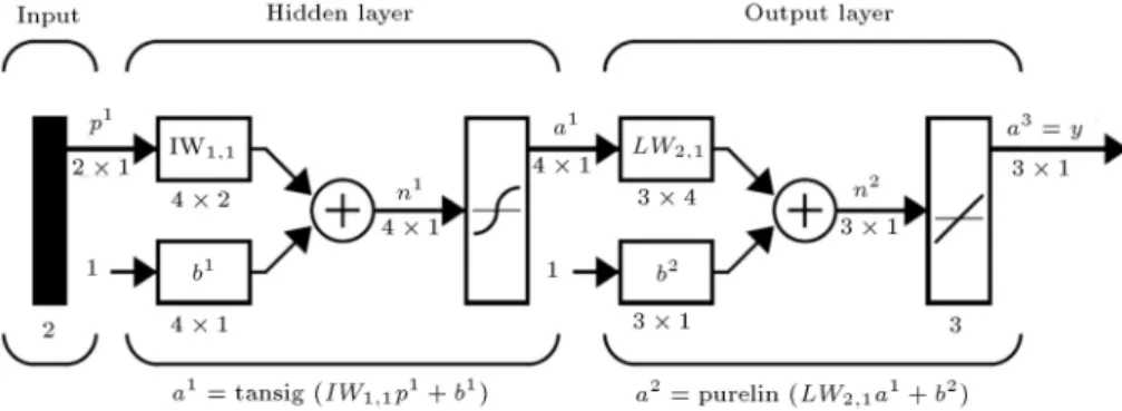
2.2. Articial Neural Networks (ANNs) ANN is a nonlinear mathematical model able to sim-ulate many mathematical complexes corresponding to inputs and outputs. Multilayer perceptron networks are common types of ANN that are widely used in studies. To use MLP model, denition of appropriate functions, weights, and bias should be considered. Due to the nature of the problem, dierent activity functions in neurons can be used. An ANN may have one or more hidden layers. Figure 1 demonstrates a three-layer neural network consisting of inputs layer, hidden layer (layers), and outputs layer. As shown in Figure 2, wi is the weight and bi is the bias
for each neuron. Weight and biases' values will be assigned progressively and corrected during training process by comparing the predicted outputs with the known outputs. Such networks are often trained using backpropagation algorithm. In the present study, ANN was trained by Levenberg-Marquardt technique, because this technique is more powerful and faster than the conventional gradient descent technique [43]. 2.3. Multivariate Adaptive Regression Splines
(MARS)
The MARS refer to a novel approach in the eld of soft computing which applies a series of simple linear regressions. As mentioned in the Introduction Section, the MARS was introduced by mathematician Friedman [33]. MARS is a high precision technique for modeling the systems based on the data set. This approach separated the computational space into sub ranges of input variables (predicting parameters) and dened the relationship between the input parameters and output variable. In other words, this technique has high ability to characterize the relationship between the independent and dependent variables in each desired phenomenon. This process was carried out by tting a simple regression into each input parameter for predicting the output. MARS separated the space of inputs parameters into various units, and then tted a spline function into these units. These elements of the regressions are named as basic function of the MARD methods. One of the main advantages of the MARS
method is highlighting the input parameters with more eect on the output parameter. This method could be used for small and big data sets. A basic function gives information about the relationship between the inputs and output parameters which is dened as:
hm(x)=Max(0; C x) or
hm(x)=Max(0; x C); (10)
where h is the basic function, x is the input parameter, C is the threshold value of the independent (input) parameter of x. The general form of the MARS is introduced as follows:
Y = f(x) = 0+ M
X
m=1
mhm(x); (11)
where Y is the output parameters, 0 is the constant
value, M is the number of function, hm(x) is the Mth
basic function, and m is the corresponding coecient
of hm(x). It takes two steps to develop the MARS. At
the rst step, all the basic functions are prepared. In this step, overtting may occur; so in the next step, to prevent overtting, the basic functions, which are of less importance, are pruned with Generalized Cross-Validation (GCV) criteria calculated in Eq. (12):
GCV = n1
Pn
i=1(yi f(xi))2
1 C(B)n 2 ; (12) where n denotes the number of observation, and C(B) (Eq. (13)) denotes a complexity criterion which increases by the number of basic functions [21]:
C(B) = (B + 1) + dB: (13)
3. Results and discussion
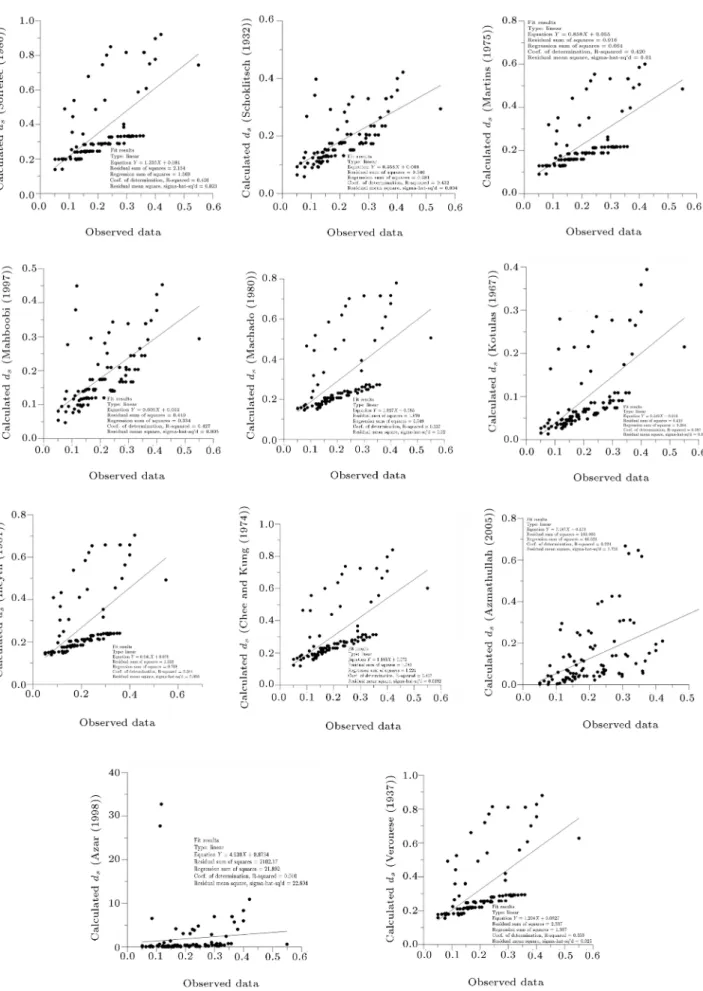
The scour depth at the downstream of ip buckets was assessed with regard to the collected data set. In other words, the value of input variables in each empirical for-mula was chosen with regard to the collected data set. The performance of empirical formula was evaluated by
calculating the standard error indices. The results of each empirical formula are plotted versus the observed data as shown in Figure 3. Moreover, In this gure, the error indices are shown. Schoklitsch (1932) with R2 =
0:45 and RMSE=0.08 is accurate among the empirical formulas, as shown in this gure, and the poorest performance is related to Azar (1998); as seen, all the empirical formulas have no acceptable performances for practical purposes. The results of assessing the performance of empirical formula support those of the study conducted by Azmathullah et al. [9] who stated that using the empirical formula for calculating the depth of scour has obvious errors compared to the measured data.
3.1. Gamma test
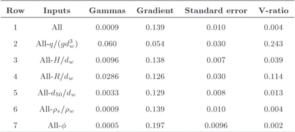
In this study, to dene the most important aective parameters on the scour at downstream of ip bucket, seven scenarios were considered. In the following, these scenarios were analyzed using the gamma test. The scenarios were considered with regard to Eq. (2). Scenario number 1 in Table 3 at row number 1 contains all the input parameters. In the following, to dene the most important parameters, one of the input parameters was removed in GT analysis. This process is continued to dene the importance of each input parameter. The results of GT analysis are presented in Table 3. The GT parameters, such as gamma, gradient, standard error, and V-ratio, were chosen as the criteria for dening the most important parameters. The scenario with the minimum value for the GT parameters shows the most aective inuence of input parameters on the output parameter. The variation of V-ratio is between 0 and 1. This point is notable in that this factor is close to zero which shows that the related scenario could accurately predict the output regarding the related input parameters.
Reviewing Table 3, it is clear that scenario num-ber 1, which involves the total input variables, has minimum value for the GT parameters. Table 3 shows that removing parameters q=(gd3
w) and R=dw causes a
Table 3. Results of gamma test analysis test.
Row Inputs Gammas Gradient Standard error V-ratio
1 All 0.0009 0.139 0.010 0.004
2 All-q=(gd3
w) 0.060 0.054 0.030 0.243
3 All-H=dw 0.0096 0.138 0.007 0.039
4 All-R=dw 0.0286 0.126 0.030 0.114
5 All-d50=dw 0.0033 0.129 0.008 0.013
6 All-s=w 0.0009 0.139 0.010 0.004
Figure 4. The variation of gamma static and standard error with unique data points.
signicant increase in the gamma value, so it is found that these parameters are the most important param-eters of the scouring depth. The variation of gamma and standard error values for the data set is shown in Figure 4, where the standard error curve and gamma curve meet at point 80. It means that for modeling the scouring depth with regard to the collected data set, qualication of 80 data sets is enough.
3.2. Articial neural network results
Developing the Articial Neural Network (ANN) mod-els, as popular representative of soft computing tech-niques, is based on the data set. So, for this purpose, the collected data set is divided into two groups as training and testing data sets. Data selections for training and testing process the ANNs model carried out by random approach. The percent of each group portfolio from the total data set will be determined during the model preparation. The input parameters were chosen with regard to Eq. (2); in other words, q=pgd3
w, H=dw, R=dw, d50=dw, and were chosen as
input variables, and ds=dw was considered as output
parameter. Designing the structure of ANNs model is almost based on the designer experience, whereas rec-ommendation of investigators who conducted similar research is useful. Designing the ANNs model includes the types of the neural network model, such as multi-layer perceptron, support vector machine radial basis
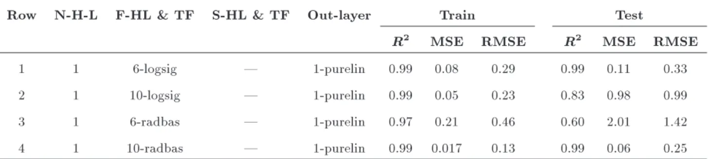
function, etc., number of the hidden layer(s), number of the neurons in each layer, dening the suitable transfer function for the neurons of hidden and output layers and learning algorithm. In this study, to assess the performance of ANNs models for modeling the scouring depth at the downstream of ip buckets, two models, such as multilayer perceptron (MLP) and Radial Basis Function (RBF) model, were applied. As mentioned in the past section, preparation of ANNs model included the number of the hidden layer, number of the neuron in each layer, type of the transfer function, and learning method. To obtain an optimal structure for the ANNs model, rstly, one hidden layer was considered; in the following, the number of the neurons in the hidden layer was increased one by one, and various types of transfer function, such as Radial Basis Function (RBF), log-sigmoid transfer (logsig), hyperbolic tangent log-sigmoid transfer (tansig), linear transfer function(purelin), etc., were tested. For developing the ANNs model, the Matlab software utilities were applied. During the ANNs models' development, it was found that the two transfer functions, RBF and logsig, have very suitable performance among the other type of transfer functions. The Levenberg-Marquardt technique was used for ANNs model learning. Table 4 presents a summary of try-and-error process conducted to dene the ANNs models with very suitable performance for predicting the scour depth at the downstream of ip bucket of spillway.
As seen in Table 4, the MLP model, which con-tained ten neurons with logsig and radbas as transfer functions, has suitable performance to model the scour depth. During the ANNs model development, it was found that the increase of the number of neurons in the rst hidden layer and adding the number of the hidden layer have no signicant eect on the increasing performance of the model. During the ANNs model preparation, it was also found that increasing the number of the neurons causes a decrease in the ANNs model performances. As seen in Table 4, adding four neurons to the existing ones in the rst hidden layer
Table 4. The performance and summary of the MLP model during the development stage.
Row N-H-L F-HL & TF S-HL & TF Out-layer Train Test
R2 MSE RMSE R2 MSE RMSE
1 1 6-logsig | 1-purelin 0.99 0.08 0.29 0.99 0.11 0.33
2 1 10-logsig | 1-purelin 0.99 0.05 0.23 0.83 0.98 0.99
3 1 6-radbas | 1-purelin 0.97 0.21 0.46 0.60 2.01 1.42
4 1 10-radbas | 1-purelin 0.99 0.017 0.13 0.99 0.06 0.25
Note: N-H-L: Number of Hidden Layer, F-HL & TF: First Hidden Layer & Transfer Function, S-HL & TF: Second Hidden Layer & Transfer Function.
Figure 5. The structure of developed MLP model with logsig function.
Figure 6. The structure of developed MLP model with radial basis function.
due to data number limitation causes a decrease in the model performance at the testing stage. The structure of the two ANNs model is shown in Figures 5 and 6.
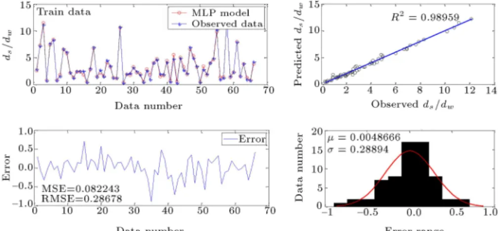
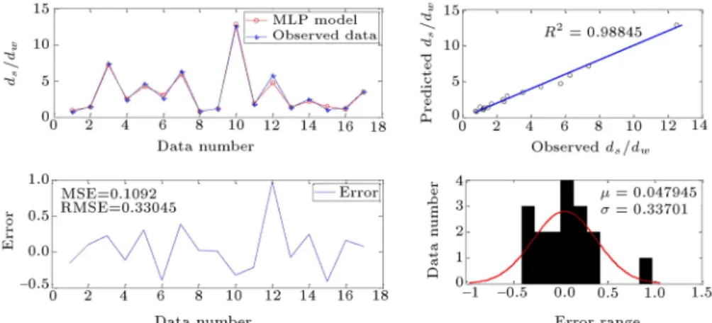
The performance of the two ANNs models during the training and testing stages is shown in Figures 7 to 10. As seen in these gures, the minimum error indices are equal to R2 = 0:95 and RMSE=0.44, and
these correspond to the RBF transfer function. In these gures, the results of the ANNS models during the training and testing stages are plotted together and compared with the observed data. To present more
information about the ANNs models' performances, the error distribution for the training and testing data sets is also plotted. Moreover, the histogram of error is plotted to dene the density of error. Evaluating the error histogram shows that most error values are concentrated around the zero.
3.3. Result of MARS model
Preparation of the MARS model as similar to other type of soft computing models is based on the data set. For this purpose, collected data set with regard to the GT results (Figure 4) and Eq. (2) was randomly divided into two groups of training and testing. 85% of the total data were considered for training and others (15%) for testing group. During the MARS model development, at the rst step, 25 basic functions were considered, and at the second step (pruning step), seven basic functions were pruned. At the end, the optimal MARS model with 18 basic functions was derived. The general form of the obtained model MARS is given in Eq. (14):
ds=dw= 6:006 + 12
X
m=1
mhm(x): (14)
The extended form of the MARS model is given in Table 5.
Note : x1 : pq gd3
w
; x2 : dH
w;
x3 : dR
w; x4 :
d50
dw;
x5 : s
w; x6 : :
Eq. (10) can be used for predicting the scour depth of a downstream of ip bucket. As seen in Table 5,
q
p
gd3 w,
H dw, and
R
dw have appeared in almost all of the
basic functions. It means that these three parameters, in comparison to the other parameters, are more
Figure 8. The performance of developed MLP model during the testing stage with logsig function.
Figure 9. The performance of developed MLP model during the training stage with radial basis function.
Figure 10. The performance of developed MLP model during the testing stage with radial basis function.
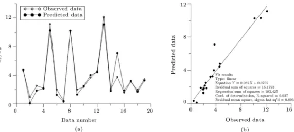
eective in the scour depth. This result from the MARS model upholds the results of the MLP model of sensitivity analysis and GT. Moreover, the performance of the MARS model during the development process (training and testing stages) is given in Figures 11 and 12, where the MARS model along and versus the observed data is plotted. Moreover, the results of error indices calculation appear in these gures; as seen, the
performance of the MARS model for predicting the scour depth is so suitable, specically when compared to the empirical formulas.
3.3.1. Comparing the results with those of the previous studies
In this section, the results of the MARS model are compared with those of other soft computing
tech-Table 5. The basic function and the related coecient of the MARS model.
Basic function Equation Coecient m
h1(x) BF 1 = max(0; 1:646 x1) -1.215
h2(x) BF 2 = max(0; x2 12:255) -218.871
h3(x) BF 3 = max(0; x4 0:08) 144.525
h4(x) BF 4 = max(0; 0:08 x4) 46.537
h5(x) BF 5 = BF 1 max(0; 0:08 x4) -6.674
h6(x) BF 6 = max(0; x3 3:204) max(0; 0:611 x6) 3.207
h7(x) BF 7 = max(0; 3:204 x3) max(0; x4 0:011) -0.146
h8(x) BF 8 = max(0; 12:255 x2) max(0; 0:835 x1) 4.067
h9(x) BF 9 = BF 4 max(0; 7:536 x2) 22.715
h10(x) BF 10 = max(0; 12:255 x2) max(0; x4 0:0137) -49.226
h11(x) BF 11 = max(0; 12:255 x2) max(0; 0:0137 x4) 22.906
h12(x) BF 12 = max(0; x4 0:0137) max(0; x2 3:015) -1.215
Figure 11. The performance of MARS model during the development stage.
Figure 12. The performance of MARS model during the testing stage.
nique implemented for predicting the scouring depth at downstream of ski-jump bucket. Goyal and Ojha [27] developed the ANN, SVM, and M5 Model Tree for predicting the scour depth at downstream of ski-jump bucket. They considered various scenarios with regard to the aective parameters during the development of mentioned soft computing techniques. They found that
when all aective parameters are considered as input parameters, the ANN is more accurate. They evaluated the performance of soft computing techniques in the absence of other aective parameters, and found that the SVM is more accurate. The results of developed MLP in this study also showed that the performance of MLP model with regard to the all input eective
pa-rameters is very suitable. Noori and Hooshyaripor [28] developed the ANN model based on the most eective input parameters, and found that the log-sigmoid has suitable performance for modeling the scour depth at downstream of ski-jump bucket, and also Azmathullah et al. [9] found that the radial basis function has suitable performance for modeling the scour depth. Na-jafzadeh et al. [37] developed the GMDH model to pre-dict the scour depth, and found that ' and H1=dware
more important parameters for predicting scour hole geometry. The results of these studies uphold those of GT and MARS models conducted on this study.
4. Conclusion
Scouring at downstream of hydraulic structures is one of the main hazards discussed in the eld of safety fac-tor analysis. Among the hydraulic structures, spillways are the most important structures, specically in the big dam projects. In the high-head dam projects, ip buckets are used for energy dissipation. Scouring at downstream of this structure is one of the ip buckets in the main hazard related to the high-head dam projects. Recently, by advancing the soft computing techniques in most areas, especially in the water engineering, using these models has been applied to predict the scouring phenomena. Today, the new soft computing mod-els, such as Multivariate Adaptive Regression Splines (MARS), have been proposed for modeling the complex systems based on the input and output data set. The results of this study showed that the MARS model has high precision for modeling the scouring depth at downstream of ip buckets. The main utilities of the MARS model are related to give clear information about internal process carried out in the development process model. Another utility of the MARS model is related to programing its results for another purpose.
References
1. Dehdar-behbahani, S. and Parsaie, A. \Numerical modeling of ow pattern in dam spillway's guide wall. Case study: Balaroud dam, Iran", Alexandria Engineering Journal, 55(1), pp. 467-473 (2016).
2. Hager, W.H. and Pster, M. \Hydraulic modelling - an introduction: Principles, methods and applications", Journal of Hydraulic Research, 48(4), pp. 557-558 (2010).
3. Parsaie, A., Haghiabi, A.H. and Moradinejad, A. \CFD modeling of ow pattern in spillway's approach channel", Sustainable Water Resources Management, 1(3), pp. 245-251 (2015).
4. Chinnarasri, C., Kositgittiwong, D. and Julien, P.Y. \Model of ow over spillways by computational uid dynamics", Proceedings of the Institution of Civil Engineers - Water Management, 167(3), pp. 164-175 (2014).
5. Muzzammil, M. and Siddiqui, N.A. \Reliability anal-ysis of scour downstream of a ski-jump bucket", Pro-ceedings of the Institution of Civil Engineers - Water Management, 162(6), pp. 389-398 (2009).
6. Zhang, H. and Zhang, X. \Numerical simulation of ski-jump jet motion using lattice Boltzmann method", Science China Technological Sciences, 54(1), pp. 72-75 (2011).
7. Heller, V., Hager, W.H. and Minor, H.-E. \Ski jump hydraulics", Journal of Hydraulic Engineering, 131(5), pp. 347-355 (2005).
8. Dargahi, B. \Scour development downstream of a spillway", Journal of Hydraulic Research, 41(4), pp. 417-426 (2003).
9. Azmathullah, H.M., Deo, M.C. and Deolalikar, P.B. \Neural networks for estimation of scour downstream of a ski-jump bucket", Journal of Hydraulic Engineer-ing, 131(10), pp. 898-908 (2005).
10. Kumar, C. and Sreeja, P. \Evaluation of selected equa-tions for predicting scour at downstream of ski-jump spillway using laboratory and eld data", Engineering Geology, 129-130, pp. 98-103 (2012).
11. Xiao, Y., Wang, Z., Zeng, J., Zheng, J., Lin, J. and Zhang, L. \Prototype and numerical studies of interference characteristics of two ski-jump jets from opening spillway gates", Engineering Computations, 32(2), pp. 289-307 (2015).
12. Najafzadeh, M. \Neuro-fuzzy GMDH based particle swarm optimization for prediction of scour depth at downstream of grade control structures", Engineering Science and Technology, an International Journal, 18(1), pp. 42-51 (2015).
13. Najafzadeh, M. and Lim, S.Y. \Application of im-proved neuro-fuzzy GMDH to predict scour depth at sluice gates", Earth Science Informatics, 8(1), pp. 187-196 (2015).
14. Najafzadeh, M. \Neuro-fuzzy GMDH systems based evolutionary algorithms to predict scour pile groups in clear water conditions", Ocean Engineering, 99, pp. 85-94 (2015).
15. Azamathulla, H.M., Haghiabi, A.H. and Parsaie, A. \Prediction of side weir discharge coecient by support vector machine technique", Water Science and Technology: Water Supply, 16(4), pp. 1002-1016 (2016). DOI:10.2166/ws.2016.014.
16. Parsaie, A. \Predictive modeling the side weir dis-charge coecient using neural network", Modeling Earth Systems and Environment, 2(2), pp. 1-11 (2016).
17. Parsaie, A. and Haghiabi, A.H. \Predicting the longi-tudinal dispersion coecient by radial basis function neural network", Modeling Earth Systems and Envi-ronment, 1(4), pp. 1-8 (2015).
18. Parsaie, A. and Haghiabi, A.H. \Prediction of dis-charge coecient of side weir using adaptive neuro-fuzzy inference system", Sustainable Water Resources Management, pp. 1-8 (2016). DOI:10.1007/s40899-016-0055-6. In press
19. Parsaie, A., Haghiabi, A.H., Saneie, M. and Torabi, H. \Prediction of energy dissipation on the stepped spillway using the multivariate adaptive regression splines", ISH Journal of Hydraulic Engineering, 22(3), pp. 281-292 (2016).
20. Ayoubloo, M.K., Azamathulla, H.M., Ahmad, Z., Ghani, A.A., Mahjoobi, J. and Rasekh, A. \Prediction of scour depth in downstream of ski-jump spillways using soft computing techniques", International Jour-nal of Computers and Applications, 33(1), pp. 92-97 (2011).
21. Samadi, M., Jabbari, E., Azamathulla, H.M. and Mo-jallal, M. \Estimation of scour depth below free overfall spillways using multivariate adaptive regression splines and articial neural networks", Engineering Applica-tions of Computational Fluid Mechanics, 9(1), pp. 291-300 (2015).
22. Najafzadeh, M. and Azamathulla, H.M. \Neuro-Fuzzy GMDH to predict the scour pile groups due to waves", Journal of Computing in Civil Engineering, 29(5), pp. 04014068 (2015).
23. Azamathulla, H.M. and Ghani, A.A. \Genetic pro-gramming for predicting longitudinal dispersion coe-cients in streams", Water Resour Manage, 25(6), pp. 1537-1544 (2011).
24. Azamathulla, H.M., Ghani, A.A. and Zakaria, N.A. \ANFIS-based approach to predicting scour location of spillway", Proceedings of the Institution of Civil Engineers - Water Management, 162(6), pp. 399-407 (2009).
25. Azamathulla, H.M., Deo, M.C. and Deolalikar, P.B. \Alternative neural networks to estimate the scour below spillways", Advances in Engineering Software, 39(8), pp. 689-698 (2008).
26. Azamathulla, M.H., Ghani, A.A., Zakaria, N.A., Lai, S.H., Chang, C. K., Leow, C.S. and Abuhasan, Z. \Genetic programming to predict ski-jump bucket spill-way scour", Journal of Hydrodynamics, Ser. B, 20(4), pp. 477-484 (2008).
27. Goyal, M.K. and Ojha, C.S.P. \Estimation of scour downstream of a ski-jump bucket using support vector and M5 model tree", Water Resources Management, 25(9), pp. 2177-2195 (2011).
28. Noori, R. and Hooshyaripor, F. \Eective prediction of scour downstream of ski-jump buckets using articial neural networks", Water Resources, 41(1), pp. 8-18 (2014).
29. Azamathulla, H.M. \Gene expression programming for prediction of scour depth downstream of sills", Journal of Hydrology, 460-461, pp. 156-159 (2012).
30. Najafzadeh, M., Etemad-Shahidi, A. and Lim, S.Y. \Scour prediction in long contractions using ANFIS and SVM", Ocean Engineering, 111, pp. 128-135 (2016).
31. Najafzadeh, M. and Bonakdari, H. \Application of a neuro-fuzzy GMDH model for predicting the velocity at limit of deposition in storm sewers", Journal of Pipeline Systems Engineering and Practice, 8(1), p. 06016003 (2017). DOI:10.1061/(asce)ps.
32. Friedman, J.H.\ Multivariate adaptive regression splines", The Annals of Statistics, pp. 1-67 (1991).
33. Samadi, M., Jabbari, E., Azamathulla, H.M. and Mo-jallal, M. \Estimation of scour depth below free overfall spillways using multivariate adaptive regression splines and articial neural networks", Engineering Applica-tions of Computational Fluid Mechanics, 9(1), pp. 291-300 (2015).
34. Sharda, V.N., Prasher, S.O., Patel, R.M., Ojasvi, P.R. and Prakash, C. \Performance of Multivariate Adap-tive Regression Splines (MARS) in predicting runo in mid-Himalayan micro-watersheds with limited data" [Performances de regressions par splines multiples et adaptives (MARS) pour la prevision d'ecoulement au sein de micro-bassins versants Himalayens d'altitudes intermediaires avec peu de donnees], Hydrological Sci-ences Journal, 53(6), pp. 1165-1175 (2008).
35. Zhang, W. and Goh, A.T.C. \Multivariate adaptive regression splines and neural network models for pre-diction of pile drivability", Geoscience Frontiers, 7(1), pp. 45-52 (2016).
36. Najafzadeh, M., Barani, G.-A. and Hessami-Kermani, M.-R. \Group method of data handling to predict scour at downstream of a ski-jump bucket spillway", Earth Science Informatics, 7(4), pp. 231-248 (2014).
37. Naghikhani, A., Noori, R., Sheikhian, H. and Ghi-asi, B. \Estimating scour hole dimensions of ski jump downstream of dams using granular computing model", Journal of Hydraulics, 9(3), pp. 45-60 (2015).
38. Noori, R., Karbassi, A. and Salman Sabahi, M. \Eval-uation of PCA and Gamma test techniques on ANN operation for weekly solid waste prediction", Journal of Environmental Management, 91(3), pp. 767-771 (2010).
39. Noori, R., Deng, Z., Kiaghadi, A. and Kachoosangi, F.T. \How reliable are ANN, ANFIS, and SVM tech-niques for predicting longitudinal dispersion coecient in natural rivers?", Journal of Hydraulic Engineering, 142(1), p. 04015039 (2016).
40. Noori, R., Karbassi, A.R., Moghaddamnia, A., Han, D., Zokaei-Ashtiani, M.H., Farokhnia, A. and Gousheh, M.G. \Assessment of input variables deter-mination on the SVM model performance using PCA, Gamma test, and forward selection techniques for monthly stream ow prediction", Journal of Hydrology, 401(3-4), pp. 177-189 (2011).
41. Moghaddamnia, A., Ghafari Gousheh, M., Piri, J., Amin, S. and Han, D. \Evaporation estimation using articial neural networks and adaptive neuro-fuzzy inference system techniques", Advances in Water Re-sources, 32(1), pp. 88-97 (2009).
42. Parsaie, A. and Haghiabi, A.H. \Computational mod-eling of pollution transmission in rivers", Applied Water Science, pp. 1-10 (2015). DOI:10.1007/s13201-015-0319-6
Biography
Amir Hamzeh Haghiabi is an Associate Professor in the Water Engineering at the Lorestan University, Lorestan Province, Iran. Dr. Haghiabi received his PhD in Hydro Structure Engineering (Water engi-neering) from Shahid Chamran University, Ahvaz in 2005. Dr. Haghiabi's research has focused on sediment transport, river meandering, numerical and physical modeling of the rivers and hydraulic structure.
![Figure 1. The ski-jump bucket spillway scour [37].](https://thumb-us.123doks.com/thumbv2/123dok_us/8377171.2225245/2.892.454.807.150.220/figure-the-ski-jump-bucket-spillway-scour.webp)
![Table 1. Summary of the famous empirical formula proposed for
ip bucket scour depth [28].](https://thumb-us.123doks.com/thumbv2/123dok_us/8377171.2225245/3.892.160.756.166.616/table-summary-famous-empirical-formula-proposed-bucket-scour.webp)