Determining Maximum Load Carrying Capacity of Flexible Link Manipulators

Determining Maximum Load Carrying

Capacity of Flexible Link Manipulators

M.H. Korayem

_{, R. Haghighi}

_{, A. Nikoobin}

_,

A. Alamdari

_{and A.H. Korayem}

Abstract. In this paper, an algorithm is proposed to improve the Maximum Load Carrying Capacity (MLCC) of exible robot manipulators. The maximum allowable load which can be achieved by a exible manipulator along a given trajectory is limited by the joints' actuator capacity and the end eector accuracy constraint. In an open-loop approach, the end eector deviation from the predened path is signicant and the accuracy constraint restrains the maximum payload before actuators go into saturation mode. By using a controller, the accuracy of tracking will improve. The actuator constraint is not a major concern and, therefore, the full power of the actuators, which leads to an increase in the Maximum Load Carrying Capacity, can be used. In this case, the controller can play an important role in improving the maximum payload, so a robust controller is designed. However, the control strategy requires measurement of the elastic variables' velocity, which is not conveniently measurable. So, a nonlinear observer is designed to estimate these variables. A stability analysis of the proposed controller and state observer is performed on the basis of the Lyapunov Direct Method. In order to verify the eectiveness of the presented method, simulation is done for a two link exible manipulator. The obtained maximum payload for open and closed-loop cases is compared, and the superiority of the method is illustrated.

Keywords: Maximum Load; Boundary layer sliding mode; Nonlinear state observer.

INTRODUCTION

Finding the full load motion for a given point-to-point task can maximize the productivity and economic usage of the manipulators. The maximum allowable load of a xed base manipulator is often dened as the maximum value of the load that a robot manipulator is able to carry on a desired trajectory which is based on a consideration of inertia eects on this desired path [1]. For rigid manipulators, the maximum load on a given trajectory is primarily constrained by the joint actuator torque and its velocity characteristic. However, for exible manipulators another constraint, i.e. maximum allowable deection, must be considered.

The maximum load carrying capacity along the given path can be determined in both open loop and closed-loop cases. In most previous works dealing with determining the DLCC along a given path, only

1. Robotic Research Laboratory, Department of Mechanical En-gineering, Iran University of Science and Technology, Tehran, P.O. Box 18846, Iran.

*. Corresponding author. E-mail: [email protected]. Received 26 June 2008; received in revised form 6 February 2009; accepted 16 March 2009

dynamic equations have been used without considering the controller, while most manipulators in industrial applications are working based on feedback. In open loop cases, several algorithms are proposed for nd-ing the maximum load carrynd-ing capacity of parallel robots [2], rigid mobile manipulators [3], exible joint manipulators [4], exible link manipulators [5], cable-suspended parallel manipulators [6] and redundant manipulators [7]. In the closed-loop case, the controller type and its parameters have a signicant eect on increasing the maximum payload. In [8], a closed-loop approach has been employed to determine the DLCC of a exible joint manipulator by considering a feedback linearization controller to track a predened path. Another work, based on a sliding mode technique, has been undertaken for exible joint manipulators in [9].

In exible link manipulators, strong coupling between the nonlinear rigid-body motions and the linear elastic displacements of the links as well as the strong coupling between the elastic displacements of the links during large motions of the manipulator, makes the dynamics of exible manipulators as highly coupled nonlinear time-varying MIMO systems with distributed parameters [10]. Complexities, such as

the non-minimum-phase property of the tip transfer function that contains unstable zeros and complex poles in this transfer function and the existence of unstructured uncertainties due to the truncation of high-order resonance modes and system nonlinearities makes it dicult to accurately position the tip of the exible manipulator [11-16]. Moreover, it creates a very challenging task in designing controllers for exible manipulators. One method that is excessively used in the control of nonlinear systems is feedback linearization [17-19]. However, for exible link robots, due to highly nonlinear coupled dynamics and the existence of passive degrees-of-freedom, only Partial Feedback Linearization (PFL) is suitable. For exible link robots, the portion of the dynamics corresponding to the active degrees of freedom can be linearized by the nonlinear feedback. The remaining portion of the dynamics after such partial feedback linearization is nonlinear and represents internal dynamics [20]. A major drawback in this method, which cannot be used solely as a controller, is its lack of robustness with respect to uncertainties.

Sliding Mode Control (SMC), as a powerful method of tackling uncertain nonlinear systems, is particularly suited for complex systems such as exible manipulators [21]. In the design of SMC, it is assumed that the control can be switched from one structure to another innitely fast. However, because of the switching delay computation and the limitation of physical actuators that cannot handle the switching of the control signal at an innite rate, it is practically impossible to achieve high-speed switching control. As a result of this imperfect control switching between structures, the system trajectory appears to chatter instead of sliding along the switching surface. Chatter involves high frequency control switching and may lead to the excitation of previously neglected high frequency system dynamics. Smoothing techniques, such as boundary layer normalization and replacement of the discontinuous control term by a fuzzy system [22,23] have been employed. The smoothing of control dis-continuity inside the boundary layer essentially assigns a lowpass lter structure to the local dynamics of the variable, s, thus eliminating chatter.

An accurate knowledge of arm state variables is required by many advanced control techniques for exible multi-link robots [24-29]. It can be conveniently achieved by using a state observer. Some works have been done using linear observers derived for a linearized model of the arm [30]. Other papers propose the use of nonlinear state observers to obtain the values of unmea-surable state variables [31-32]. In exible manipulators, it is possible to measure joint positions, velocities and exible modes of manipulators using shaft encoders, tachometers and strain gauges, respectively. However, measuring the exural generalized velocities cannot

be easily or accurately accomplished. Thus, a state observer is desirable in these circumstances. In order to decrease computational eort, a reduced order ob-server for estimating only exible variables can be very helpful. The observer is designed based on a sliding mode approach. Similar to sliding mode controllers, sliding mode observers are designed by using sliding surfaces and oer robustness against both parametric uncertainties and external disturbances. The proposed observer requires positions and velocities of joints as well as exible modes, and it estimates the rates of change of exible modes.

An industrial manipulator usually requires six Degrees Of Freedom (DOF) in order to eciently drive the gripper to a specied position with a prescribed orientation in the workspace. If it is constructed as a lightweight manipulator, practically, only the two-DOF rotary long links will be deformed under heavy loading and fast motion. So, the simulation is done for a two link exible manipulator. In order to show the eectiveness of the proposed closed-loop algorithm, the simulation is done for both open loop and closed-loop cases. In closed-closed-loop cases, the controller and the observer have been designed based on the rst elastic mode of the beam, while the dynamic model is based on two elastic modes of the beam. The second elastic mode has been included to investigate the eects of unstructured uncertainties on the overall performance of the closed-loop system.

The paper is organized as follows: First, the gen-eral dynamic equations of a exible link manipulator are derived. Then, by using partial feedback lineariza-tion, a controller is designed for a partially linearized model of a exible manipulator based on a sliding mode approach. Following that, an algorithm is proposed to compute maximum allowable load by considering the limiting factors. Finally, some numerical result is shown.

DYNAMICS OF FLEXIBLE-LINK MANIPULATOR

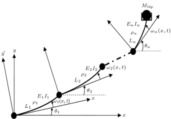
Assuming that each arm does not undergo torsional deformations and considering an Euler-Bernoulli beam for each link, exible-link robotic manipulators can be described as innite-dimensional dynamical systems by using partial dierential equations [33] (see Figure 1). In order to derive a nite-dimensional ordinary dif-ferential equation, an approximation approach using assumed mode methods, is taken into account.

By applying the Lagrange formulation, the dy-namics of any multi-link exible-link robot can be represented by:

Figure 1. Flexible manipulator.

where q(t) = [qT

r; qfT]T, in which qris the vector of rigid

modes (generalized joint coordinates) and qf is the

vector of exible modes. M(q) represents the inertia matrix, N(q; _q) is a n 1 vector of centripetal and Coriolis velocity terms.

The exible manipulator dynamics are parti-tioned into rigid and exible degrees-of-freedom as:

(

Mrrqr+ Mrfqf+ Nr= u I

Mfrqr+ Mffqf+ Nf = 0 II (2)

where the following properties are known to be veried by the Lagrangian structure denite matrices.

Properties

I. M(q); Mrr(q) and Mff(q) are non-singular,

sym-metric, positive denite matrices.

II. Mrr+MrfMff1Mfris a symmetric positive-denite

matrix.

CONTROLLER DESIGN

The controller design of a exible link manipulator is divided into two steps. First, by applying partial feedback linearization, the dynamic of the exible link is divided into two parts: a partially linearized model and an internal model. Second, use of the sliding mode approach forces the state trajectory of a system to the origin in the error phase hyperplane during two distinct phases: reaching phase and sliding phase.

Partial Feedback Linearization

For exible manipulators that have a passive degree, instead of applying fully feedback linearization, it is convenient to use partial feedback linearization. The formulation of partial feedback linearization is as fol-lows.

From Equation 2-II, qf can be expressed as below:

qf = Mff1[Mfrqr Nf]: (3)

Substituting for qf from Equation 3 in Equation 2-I

gives:

[Mrr+ MrfM_ff1Mfr]qr+ Nr MrfM_ff1Nf = u:

(4) It can be easily seen that Equation 4 is similar in form to rigid manipulator modeling with the equivalent symmetric and positive denite mass matrix, Mrr +

MrfM_ff1Mfr, based on property II. The zero dynamic

is dened for a nonlinear system Equation 2 by putting qrand its derivatives equal to zero. So:

Mffqf+ Nf = 0; (5)

where Nf is simplied to Kqf where:

K = diagf!2

11; !122 ; : : : ; !ij2; ; !2nmg: (6)

So, Equation 5 can be written as:

Mffqf+ Kqf = 0: (7)

Since Mff and K are the positive denite symmetric

matrices, the equilibrium point [qf; _qf] of Equation 7 is

stable in the sense of Lyapunov but not asymptotically stable.

Sliding Mode Design

In the sliding-mode control theory, control dynamics have two sequential modes; the rst is the reaching mode and the second is the sliding mode. In particular, the Lyapunov sliding condition forces system states to reach a hyperplane and keeps them sliding on this hy-perplane. Essentially, a SMC design is composed of two phases: hyperplane design and controller design. There are various methods for designing hyperplane [34], however, in this paper, a method proposed by Slotine is used [35]. In this method, the sliding surface is dened as:

s = ( _~qr+ 0_~qf) + (~qr+ 0~qf); (8)

where ~qr = qr qrref and ~qf = qf qref_f . qrefr is the

desired trajectory of joints and q_fref = 0 because the desired value for exible variables is zero. Also, and 0 _{are positive constants.}

To determine the control law, the derivative of the sliding surface must be determined.

_s = (~qr+ 0~qf) + ( _~qr+ 0_~qf): (9)

Treating the term 0_~q

f as disturbance, Equation 9 is

rearranged as below:

Since the sliding condition is dened by:

_s K sign(s); (11)

so, Equation 10 in order to satisfy the sliding condition must be written as:

qr qrref+ ( _~qr+ 0_~qf) = K sign(s): (12)

By substituting qr from Equation 4, Equation 12

becomes:

[Mrr+ MrfMff1Mfr] 1[u Nr MrfMff1Nf]

(qref

r ( _~qr+ 0_~qf) = K sign(s): (13)

By extracting u from Equation 13, the control law is dened as:

u = M[qref

r ( _~qr+ 0_~qf) K sign(s)] + N; (14)

where M = [Mrr + MrfMff1Mfr] and N = Nr

MrfM_ff1Nf. From the practical point of view, deriving

the exact model of the system is a hard task, so it is convenient to use the nominal model. By dening the

^

M and ^N which are the nominal values of M and N, respectively, the control law can be rewritten as follows:

u = ^M[qref

r ( _~qr+ 0_~qf) K sign(s)] + ^N: (15)

Stability Analysis of SMC

For purpose of design integrity, a simple stability anal-ysis based on the Lyapunov Direct method is carried out. The Lyapunov function candidate is dened as follows:

V = 1₂s2_{: (16)}

Dierentiating Equation 16 and using Equations 4, 11 and 15, one can write:

_V =s_s = sfM 1_{[ ^M[q}ref

r ( _~qr+ 0_~qf)

K sign(s)]+ ^N N] qref

r ( _~qr+ 0_~qf)g: (17)

By using simplication, Equation 17 becomes: _V =sfM 1_M[q^ ref

r ( _~qr+ 0_~qf) K sign(s)]

+M 1_{N q}ref

r ( _~qr+ 0_~qf)g: (18)

For stability _V must be negative. Since _V = s _s another condition that assures the stability of the system can be dened as s _s jsj or _s sign(s) which is called

a sliding condition. By applying the sliding condition, we have:

(M 1_{M^ I)(q}ref

r ( _~qr+ 0_~qf))

M 1_{M:K:sign(s) + M^} 1_{N :sign(s): (19)}

By multiplication of both sides of Equation 19 by ^

M 1_{M, one gets:}

(I M^ 1_M)(qref

r ( _~qr+ 0_~qf))

K:sign(s) + ^M 1_{N M^} 1_{M:sign(s): (20)}

So, the condition which guarantees the stability can be expressed as follows:

K >j(I M^ 1_M)(qref

r ( _~qr+ 0_~qf))

+ ^M 1_{Nj + ^M} 1_{M: (21)}

Since M is unknown, one can dene the following known bounds:

Mmin M Mmax: (22)

Since M acts multiplicatively in the dynamics of the manipulator, it is reasonable to choose the estimate ^M of M as the geometric means of the above bounds [35]:

^

M = (MminMmax)1=2: (23)

Therefore, the bounds for ^M 1_{M can be dened as}

follows:

1 _^M 1_{M ; (24)}

where: =

Mmax

Mmin

1=2

: (25)

So, Equation 21 can be rewritten in terms of : K >j(I )(qref

r ( _~qr+0_~qf))+ ^M 1Nj+ :

(26) Boundary Layer

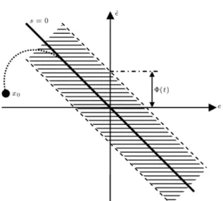
An essential drawback of SMC is that owing to the signum term, it causes abrupt changes (chattering) to the control signal, u. However, this can be avoided by introducing a boundary layer () from both sides of the sliding surface, s = 0, as shown in Figure 2.

By applying a boundary layer at both sides of the sliding surface, Equation 15 is written as below:

u = ^Mhqref

r ( _~qr+ 0_~qf) K sat s

i + ^N;

Figure 2. Variable boundary layer.

where \sat" is saturation function. If we rewrite _s based on the \sat" function, we have:

_s =(M 1_{M^ I)(q}ref

r ( _~qr+ 0_~qf))

M 1_M:K:sat^ s

+ M 1_{N: (28)}

By considering the system trajectories inside the boundary layer:

_s =(M 1_{M^ I)(q}ref

r ( _~qr+ 0_~qf))

M 1_M:K:^ s

+ M 1_{N; (29)}

and Equation 29 can be rewritten as: _s+M 1M:K^ s = (M 1_{M^ I)}

(qref

r ( _~qr+ 0_~qf)) + M 1N: (30)

In fact, Equation 30 shows that the smoothing of con-trol discontinuity inside the boundary layer essentially assigns a low pass lter structure to the local dynamics of the variable, s, thus, eliminating chattering. Fur-thermore, the sliding condition is redened as below:

_s ( _ K)sign(s): (31)

In the presence of a boundary layer, we need to guarantee that the distance from the boundary layer always decreases. System robustness is a function of the boundary layer; in other words, a thinner boundary layer gives more robust control, but larger chattering. STATE OBSERVER DESIGN

In the control law (Equation 15), measurements of the velocity of elastic variables are needed and since it

cannot easily be measured, there is a demand to design a state observer for the measuring of these variables. By extracting qr from Equation 2-I, and substituting

in Equation 2-II, we have:

MfrMrr1[u Mrfqf Nr] + Mffqf+ Nf = 0; (32)

and it can be rearranged to:

[Mff MfrMrr1Mrf]qf+ Nf MfrMrr1Nr

+ MfrMrr1u = 0: (33)

Equation 33 can be expressed in state space form: 8

< :

_xf1 = xf2

_xf2 =[Mff MfrMrr1Mrf] 1

[ Nf+ MfrMrr1Nr MfrMrr1u]

(34) where xf1 = qf and xf2= _qf.

Using a sliding mode observer technique, the dynamic of the observer is written as:

(

_^xf1 = ^xf2+ k11~xf1+ k12sign(~xf1)

_^xf2 = ^f(xr; xf1; ^xf2) + k21~xf1+ k22sign(~xf1) (35)

where ^f(xr; xf1; ^xf2) = [Mff MfrMrr1Mrf] 1[ Nf+

MfrMrr1Nr MfrMrr1u] and kij are positive

parame-ters. ~xf1 is the estimation error and equal to xf1 ^xf1.

The dynamic of error is achieved by subtracting Equation 34 from Equation 35:

(

_~xf1 = ~xf2 k11~xf1 k12sign(~xf1)

_~xf2 = ~f k21~xf1 k22sign(~xf1)

(36) where it can be written in the following simple form:

_e = ~f _K

ee Kssign(e); (37)

where ~f ₌

~xf2

~ f

and e =

~xf1

~xf2

. Using Taylor expansion around e = 0, Equation 37 can be given as:

_e = Ae + O(e2_{) K}

ssign(e); (38)

where:

A = @ ~_@ef Ke

!

e=0

= "

0 1

@ ~f

@ ~x_f1 ~xf1=0 @ ~x@ ~f_f2 ~xf2=0

# +

k11 0

k21 0

: (39) The eigenvalues of A can be specically placed by properly choosing Ke. If matrix A has negative

eigenvalues (it must be a negative denite matrix), then the error will converge to zero.

From matrix algebra, we know that a square ma-trix is negative denite if determinants of all principal minors have the following pattern:

jD1j < 0; jD2j > 0; jD3j < 0; ; (40)

where Di is the ith principle minor. So, by applying

the above conditions, we have: k11_@~x@ ~f

f2

~xf2=0+ k21

@ ~f @~xf1

~xf1=0

> 0: (41) It can be easily seen that, if k21 is chosen big enough,

the above condition is satised.

DETERMINING MAXIMUM LOAD CARRYING CAPACITY

The maximum allowable load of a xed base manipu-lator is often dened as the maximum payload that can be carried by the manipulator with acceptable accuracy. For rigid manipulators, it can be seen that MLCC is directly in relation to actuator strength, while for exible manipulators additional constraints must be considered and that is maximum allowable deection which depends on exible variables.

The above condition can be taken into account in MLCC determination by imposing a constraint on the end eector deection, in addition to the actua-tor actua-torque constraint imposed for rigid manipulaactua-tors. Deection of the end eector can cause excessive deection from the pre-dened trajectory, even though the joint torque constraints are not violated. By consid-ering the actuator torque and deection constraints and adopting a logical computing method, the maximum load-carrying capacity of a exible manipulator for a pre-dened trajectory can be computed.

MLCC can be obtained in either open loop or closed-loop cases. In open loop, the controller is not considered, and only a dynamic equation is used. In closed-loop cases, MLCC is obtained, while both the dynamic equation and controller are considered. The actuator torque constraint is formulated on the basis of the typical torque-speed characteristics of DC motors:

(

U = K1 K2_q

L = K1 K2_q (42)

where U and L are the upper bound and the lower

bound of the actuator constraint, respectively. The coecients Ki are dened as:

(

K1= Ts

K2= _!T_nls (43)

where Ts is the stall torque and !nl is the maximum

no-load speed of the motor.

In the following sections, determining the MLCC is presented for these two cases.

Determining MLCC in Open Loop Case

For computing the maximum load carrying capacity in an open loop condition, the following steps must be taken:

1. Determining the actuator path within which the arms are in fully extended congurations;

2. Finding qr; _qr; qrby solving the inverse dynamic for

the same rigid manipulator;

3. Determining qf; _qf; qf from Equation 2-II;

4. Computation of the actuators torque (nl) and end

eector path for a no load manipulator; 5. Choosing an initial value for mmax;

6. Putting mp = mmax and computing the actuators

torque (l) and end eector path;

7. Compute the actuators bounds based on Equa-tions 42 and 43;

8. Determining the load coecient Ca based on

actu-ator constraints [8]:

Ca =min(min(Carst joint(1 : n));

min(Csecond joint

a (1 : n))): (44)

9. Determining the load coecient Cp based on

accu-racy constraints:

Cp(k) = _max(Rp e(k)

e(k)) max(n(k)); (45)

where e(k) is the error of the end eector in the

presence of load and n(k) is the error of the end

eector without load.

10. Determining the load coecient C

C = min(Cp; Ca): (46)

11. If jCi+1 _Ci_{j error then m}

max = C mp,

otherwise mp= C mpand go to 6.

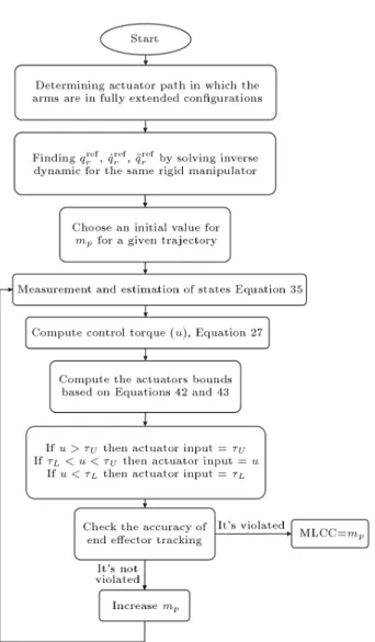
Determining MLCC in Closed-Loop Case The algorithm used for nding MLCC in closed-loop cases, as shown in Figure 3. In closed-loop cases, the actuator constraint is the major parameter in determining MLCC, while in open loop cases the end eector accuracy is the major parameter in determining MLCC. The desired path is chosen the same as in open loop cases to compare these two cases. Since in

Figure 3. Flowchart of computing dynamic load carrying capacity.

closed-loop cases the system input is computed by a controller for applying the actuator constraints instead of dening the load coecient, we put a constraint on the controller output such that, if controller output doesn't violate the actuator constraint, the system input is equal to controller output, otherwise, it is equal to the bounds of actuator constraints.

The accuracy constraint is checked by the distance between the desired and actual trajectory, which must not violate the accuracy constraint.

As can be seen, the controller plays a major role in determining the maximum load carrying capacity; in other words, improvement in controller leads to increasing MLCC.

SIMULATION STUDIES

To investigate the proposed algorithm, some simulation studies are presented for a two link exible manipu-lator. In these studies, a specied trajectory for the load is assumed. Note that the second elastic mode

is included in the model to investigate the eects of unstructured uncertainties on the overall performance of the closed-loop system. By applying the proposed algorithm for a closed-loop plant, the maximum allow-able load was computed to be mload= 4:51, meanwhile,

the maximum allowable loop for an open loop in three iterations was found to be mload = 3:63. The

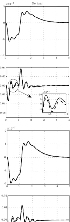
simulation results are shown in Figures 4 to 7. The parameters used in the simulation are given in Table 1. Figure 4 shows the elastic variables in an open loop case, wherein these variables do not converge to zero. Figure 5 shows that in a closed loop case, the capacity of the actuators is better in comparison to the open loop case. Figure 6 shows the good performance of the state observer in estimating elastic variable velocities. Moreover, it shows the convergence of exible link vibrations. Figure 7 shows the elastic variables used in the dynamic of the system, but in the controller and observer design, it is neglected to show the robustness of the controller, with respect to unstructured uncertainties.

Another simulation is done for a exible robot manipulator with less rigidity. The parameters of the simulation are shown in Table 2. In this case, the

Figure 4. Flexible mode shapes in open loop case.

Figure 5. Control torque in two cases; open loop (solid thin line) and closed-loop (dashed thick line).

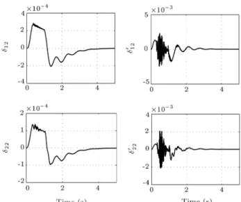
Figure 6. Flexible mode shapes in two cases (without load and full load); the actual signal is shown in solid thin line and the estimated variables are shown in dashed thick line (closed-loop case).

Figure 7. Flexible mode shapes considered only in plant (closed-loop case).

Table 1. Parameters of the simulation.

Parameter Value Unit Length of links L1= L2= 1 m

Density 1 = 2= 4:68 kg/m

Flexural rigidity E1I1= E2I2= 1025 N.m2

Actuator stall torque Ts1= 66; Ts2= 29 N.m

Actuator no-load speed !n1= !n2= 3:5 Rad/s

Controller constants = 10; K = 25 Observer constants k11= 100, k12= 1e5

k21= 100, k22= 1e5

Table 2. Parameters used for simulation.

Parameter Value Unit Length of links L1= L2= 1 m

Density 1 = 2= 4:68 kg/m

Flexural rigidity E1I1= E2I2= 100 N.m2

Actuator stall torque Ts1= 46, Ts2= 19 N.m

Actuator no-load speed !n1= !n2= 3:5 Rad/s

maximum load carrying capacity computed as mload=

2:74 in open loop and as mload = 3:87 in closed loop.

The simulation result is shown in Figures 8 and 9. CONCLUSION

The main objective of this investigation was to deter-mine the maximum load for a exible link manipulator in the presence of a controller. Therefore, in this case,

Figure 8. Control torque in two cases; closed-loop (solid thin line) and open loop (dashed thick line).

Figure 9. End eector path in two cases; open loop and closed-loop.

except for actuator constraints, end eector accuracy should be considered. The controller is designed based on a sliding mode method, and for alleviation of the chattering phenomena a boundary layer is used. However, in a control law, the velocity of the elastic variables, which cannot be measured easily, is used. So, a nonlinear state observer is designed based on a sliding mode approach to estimate these variables. The controllers and the observer have been designed in this study, based on a simplied version of the model of the arm in which only the rst elastic mode of the link is taken into account, while for the model, the second mode shape is also considered in order to investigate the eects of unstructured uncertainties on the overall performance of the closed-loop system. By applying the proposed algorithm for a closed-loop case, the maximum allowable load computed as mload = 4:51,

meanwhile, the maximum allowable loop for open loop was found as mload= 3:63.

REFERENCES

1. Yao, Y.L., Korayem, M.H. and Basu, A. \Maximum allowable load of exible manipulators for given dy-namic trajectory", Robotics and Computer-Integrated Manufacturing, 10(4), pp. 301-309 (1993).

2. Korayem, M.H. and Shokri, M. \Maximum dynamic load carrying capacity of a 6UPS-stewart platform manipulator", Scientia Iranica, 15(1), pp. 131-143 (2008).

3. Korayem, M.H., Ghariblu, H. and Basu, A. \Maximum allowable load of mobile manipulators for two given end points of end eector", International Journal of Advanced Manufacturing Technology, 24(9-10), pp. 743-751 (2004).

4. Korayem, M.H. and Nikoobin, A. \Maximum payload for exible joint manipulators in point-to-point task using optimal control approach", International Journal of Advanced Manufacturing Technology, 38(9-10), pp. 1045-1060 (2008).

5. Korayem, M.H., Heidari, A. and Nikoobin, A. \Maxi-mum allowable dynamic load of exible mobile manip-ulators using nite element approach", International Journal of Advanced Manufacturing Technology, 36(5-6), pp. 606-617 (2008).

6. Korayem, M.H. and Bamdad, M. \Dynamic load-carrying capacity of cable-suspended parallel manip-ulators", International Journal of Advanced Manufac-turing Technology, 44(7-8), pp. 829-840 (2009). 7. Korayem, M.H. and Nikoobin, A. \Maximum payload

path planning for redundant manipulator using indi-rect solution of optimal control problem", Interna-tional Journal of Advanced Manufacturing Technology, 44(7-8), pp. 725-736 (2009).

8. Korayem, M.H., Davarpanah, F. and Ghariblu, H. \Load carrying capacity of exible joint manipulators with feedback linearization", International Journal of Advanced Manufacturing Technology, 29(3-4), pp. 389-397 (2006).

9. Korayem, M.H. and Pilechian, A. \Maximum allow-able load of elastic joint robots: Sliding mode control approach", Amirkabir Journal of Science & Technol-ogy, 17(65), pp. 75-82 (2007).

10. Chen, W. \Dynamic modeling of multi-link exi-ble robotic manipulators", Computers and Structures, 79(2), pp. 183-195 (2001).

11. Oke, G. and Istefanopulos, Y. \Tip position control of a two-link exible robot manipulator based on nonlinear deection feedback", Chaos, Solitons and Fractals, 17(2), pp. 499-504 (2003).

12. Zhang, N., Feng, Y. and Yu, X. \Optimization of terminal sliding control for two-link exible manipu-lators", Proc. of IECON Industrial Electronic Confer-ence, 2, pp. 1318-1322 (2004).

13. Ho, M.T. and Tu, Y.W. \Position control of a single-link exible manipulator using H8-based PID control", IEE Proc.: Control Theory and Applications, 153(5), pp. 615-622 (2006).

14. Halevi, Y. and Nachshoni, C.W. \Transfer function modeling of multi-link exible structures", Journal of Sound and Vibration, 296(1-2), pp. 73-90 (2006). 15. Maouche, A.R. and Attari, M. \Hybrid control

strat-egy for exible manipulators", IEEE International Symposium on Industrial Electronics, pp. 50-55 (2007). 16. Fan, T. and de Silva, C.W. \Dynamic modelling and model predictive control of exible-link manipulators", International Journal of Robotics and Automation, 23(4), pp. 227-234 (2008).

17. Yang, T.W., Xu, W.L., Tso, S.K. and Vincent, T.L. \Dynamic modeling based on real-time deection mea-surement and compensation control for exible multi-link manipulators", Dynamics and Control, 11(1), pp. 5-24 (2001).

18. Benosman, M. and Le Vey, G. \Control of exible manipulators: A survey", Robotica, 22(5), pp. 533-545 (2004).

19. Kermani, M.R., Moallem, M. and Patel, R.V. \Study of system parameters and control design for a exible manipulator using piezoelectric transducers", Smart Materials and Structures, 14(4), pp. 843-849 (2005). 20. Arisoy, A., Gokasan, M. and Bogosyant, S. \Sliding

mode based position control of a exible-link arm", 12th International Conference on Power Electronics and Motion Control, pp. 402-407 (2007).

21. Perruquetti, W. and Barbot, J.P. \Sliding mode con-trol in engineering", Marcel Deckker, New York (2002). 22. Derbel, N. and Alimi, A.M. \Design of a sliding mode controller by fuzzy logic", International Journal of Robotics and Automation, 21(4), pp. 241-246 (2006). 23. Thinh Ngo, H.Q., Shin, J.H. and Kim, W.H. \Fuzzy

sliding mode control for a robot manipulator", Arti-cial Life and Robotics, 13(1), pp. 124-128 (2008). 24. Li, Y.F. and Chen, X.B. \End-point sensing and state

observation of a exible-link robot", IEEE/ASME Trans. on Mechatronics, 6(3), pp. 351-356 (2001). 25. Zaki, A., ElBeheiry, E.S. and ElMaraghy, W. \Variable

structure observer design for exible-link manipulator control", Transactions of the Canadian Society for Mechanical Engineering, 27(1-2), pp. 107-129 (2003). 26. Parsa, K. \Dynamics, state estimation, and control of

manipulators with rigid and exible subsystems", PhD Dissertation, McGill University (2003).

27. Zuyev, A. and Sawodny, O. \Observer design for a exible manipulator model with a payload", Proc. of the IEEE Conference on Decision and Control, pp. 4490-4495 (2006).

28. Caracciolo, R., Richiedei, D. and Trevisani, A. \Design and experimental validation of piecewise-linear state observers for exible link mechanisms", Meccanica, 41(6), pp. 623-637 (2006).

29. Tavasoli, A., Eghtesad, M. and Jafarian, H. \Two-time scale control and observer design for trajectory tracking of two cooperating robot manipulators mov-ing a exible beam", Proc. of the American Control Conference, 9-13, pp. 735-740 (2007).

30. Zuyev, A.L. \Observability of a exible manipulator with a payload", Physics and Control, 24-26, pp. 523-526 (2005).

31. Nguyen, T.D. and Egeland, O. \Observer design for a exible robot arm with a tip load", American Control Conference, 2(8-10), pp. 1389-1394 (2005).

32. Chalhoub, N.G. and Kfoury, G.A. \Development of a robust nonlinear observer for a single-link exible manipulator", Nonlinear Dynamics, 39(3), pp. 217-233 (2005).

33. Lee, S.H. and Lee, C.W. \Hybrid control scheme for robust tracking of two-link exible manipulator", Journal of Intelligent and Robotic Systems, 32(4), pp. 389-410 (2001).

34. Nguyen, D.K. \Sliding mode control: Advanced design

techniques", PhD Dissertation, University of Technol-ogy, Sydney, Australia (1998).

35. Slotine, J.J. and and Li, W. \Applied nonlinear con-trol", Prentice-Hall, Englewood Clis, NJ (1991).