A Genetic Algorithm for Resource
Investment Problems, Enhanced
by the Revised Akpan Method
S. Shadrokh
and F. Kianfar 1
In this paper, a genetic algorithm for solving a class of project scheduling problems, called Resource Investment Problems, is presented. Tardiness of the project is permitted with a dened penalty. The decision variables are the level of resources and the start times of the activities. The objective is to minimize the sum of resources and delay penalty costs, subject to the activities' precedence relations and some other constraints. A revised form of the Akpan heuristic method for this problem is used to nd better chromosomes. Elements of the algorithm, such as chromosome structure, untness function, crossover, mutation, immigration and local search operations, are explained. The performance of this genetic algorithm is compared with that of other published algorithms for Resource Investment Problems. Also, more than 700 problems are solved using an enumerating algorithm and their optimal solutions are used for the performance tests of the genetic algorithm. The tests results are quite satisfactory.
INTRODUCTION
The Resource Constrained Project Scheduling Problem (RCPSP) is one of the main branches of project scheduling. Some other types of scheduling problem, such as Flow-Shop and Job-Shop, can be modeled as RCPSP (see, for example, 1]). A Resource Investment Problem (RIP) is a RCPSP in which the cost of total resources used for the project is part of the objective function, which should be minimized. Mohring 2] has discussed this problem and shows that RIP is NP-hard. He considers a tight deadline for the project completion time. It is more realistic to permit project tardiness and assign a positive penalty to each unit of time delay. In this paper, RIP is considered under the condition that delay is permissible. Since scheduling problems are usually Np-hard, heuristic algorithms, such as Genetic Algorithms (GA), have gained considerable attention in recent years. For example, Hartmann 3] uses GA for Multiple Mode Resource Constrained Project Scheduling (MMRCPSP).
In this paper, a genetic algorithm for a Resource
*. Corresponding Author, Faculty of the Ghazvin Azad University, Ghazvin, I.R. Iran.
1. Department of Industrial Engineering, Sharif University of Technology, Tehran, I.R. Iran.
Investment Problem is presented, which is an enhance-ment of the authors' previous work on this problem. Tardiness in the project nishing time is permitted with a dened penalty. Whereas in the previous genetic algorithm each chromosome consisted of two parts, one for determination of start times and the other for the level of resources, in the new algorithm, chromosomes have only one part, which gives the sequence of the activities to be scheduled. Using a revised version of the Akpan method, the schedule and resource capacities for the chromosomes are, subse-quently, determined. Elements of the algorithm, such as chromosome structure, untness function, crossover, mutation and immigration operations, are explained.
To adjust the parameters of the genetic algorithm and also to test the performance, 720 problems were solved to optimality, using an enumeration process. Also, the published results of the other algorithms are compared against the performance of the genetic algorithm.
PROBLEM DESCRIPTION
There is a set of V = f01:::nn+ 1g activities
in a project that should be completed before a pre-determined deadline, T. Otherwise, with a constant
of penalty must be paid. The precedence relations of activities are shown by activity on the node network with no loops that has n+ 2 nodes. Nodes 0 and n + 1, the initial and terminal nodes, respectively,
are dummies. A set K of renewable resources,
each at a constant level, is allocated to this project. It means that, after determination of the resource levels, they remain constant during project execution. Activities are not preemptive and have one mode of execution with a constant rate of consumption of each resource during execution time. All parameters are deterministic. The problem is to nd the start time of activityiSii= 0:::n+ 1, given the resource level Rkk= 1:::, such that the precedence relations of
activities are satised and the total cost of all resources, plus delay penalties are minimized. Let:
Ck = cost of each unit of available capacity for
resourcek(k2K),
Pi = set of predecessors of activityi,
rik = rate of thekth resource usage by activityi, Di = ith activity duration time,
xit = 1, if activityistarts at timetand 0
otherwise. ThenSi=
T
P
t=0
txit and the model is as follows 4]:
min
( X
k=1
CkRk+Cdmaxf0Sn +1
;Tg )
(1)
T
X
t=0
txitDj+
T
X
t=0
txjt
j2Pi i= 1n+ 1 (2)
n
X
i=1
t
X
u=t;D i
+1
rikxiu Rk
t= 0T k2K=f1pg (3) Si=
T
X
t=0
txit i= 1n+ 1 (4)
T
X
t=0
xit= 1 i= 1n+ 1 (5) x
01= 1
(6)
xit2f01g i= 1n+ 1 t= 0T (7)
Rk 0 k2K=f1pg (8)
The objective (Formula 1) is to minimize the total cost of all resources and the probable penalties. If project nish time is within the deadline, the objective function is equal to P
k=1
CkRk, otherwise it is P
k=1
CkRk + Cd(Sn
+1
;T). Constraint in Formula 2 takes into
consideration the precedence relation between each pair of activities (ij), where j immediately precedes i. The constraint set in Statement 3 limits the total
resource usage within each period to the available amount. Constraint in Equation 4 calculates the start times. Constraint in Formula 5 guarantees that each activity, i, can only have one start time. Sets of
constraints in Formulae 7 and 8 denote the domain of variables. Shadrokh and Kianfar 5] called the above problem a resource investment problem, while tardiness is permitted (RIPT).
GENETIC ALGORITHM
Basic Scheme
The New Genetic Algorithm (NGA) uses a combina-tion of the Shadrokh and Kianfar Genetic Algorithm (SKGA) 5] and the Akpan Algorithm (AA) 6]. The basic scheme of NGA is similar to that of SKGA. Each chromosome in SKGA has two sections, an activity list section and a resource capacity list section. In NGA, each chromosome has one section, i.e., activity list, and the resource capacities are computed using a modied version of AA that was derived from AA, so that it could be applicable to RIPT. Each chromosome gives a unique value to the decision variables, Sis and Rks
of RIPT and, hence, species a unique schedule. The basic scheme of the algorithm is as follows.
Each individual within the rst generation is created randomly and its untness is calculated. Size of population, POP, is a parameter of the algorithm and remains constant for all generations. Each new generation is made from existing generations by using three operations: Crossover, mutation and immigra-tion. In the crossover operation, the existing generation is randomly partitioned into POP/2 pairs of parents and, on each pair, the crossover operation is performed with probability Pcr. If a pair is not selected for
crossover, each individual in the pair is considered for the mutation operation with probability Pmu. The
crossover operation on a pair of parents,Pa 1and
Pa 2,
gives two children, CH1and CH2. Let
f(I) be the
un-tness value of individualI. If (f(Pai)+f(CHi))ri f(Pai), then, CHi will go to the new generation and Pai dies out (i = 12), where ri is a random number
generated from the interval 0,1] for each i, otherwise
CHi dies out andPai is considered for mutation with
probability Pmu. After constructing each generation
by these operations, the immigration operation is also performed before the cycle of producing the new
generation is nalized. In the immigration operation, an immigrating chromosome is generated randomly, which is called a new chromosome. An individual
I, is randomly selected from the current population.
LetP leave(
Inew) =f(I)=(f(I) +f(new)). A random
number, r, is generated in the interval 0,1]. If r < P
leave(
Inew), immigrant new replaces I, otherwise,
new is discarded. The immigration operation gives a chance for the non-existing desirable characteristics in a population to come to it. The number of generations created for solving a problem is a parameter of the algorithm and is adjustable. The chromosome with the least untness value in the nal generation is the solution given by the algorithm. Note that POP,
Pmu and Pcr are also adjustable parameters of the
algorithm.
Chromosome Structure and Untness Function
In each generation, each individual, I, is a unique
solution to RIPT and is represented by its chromosome as: I = (jI
0
jIn
+1). Here,
jIi(i = 0:::n+ 1) is
the number of the activity, which is the ith activity
in the scheduling sequence. As noted in the section of Basic Scheme, this chromosome doesn't contain a resource capacity section, like SKGA. The order of activities from left to right in the chromosome string is such that all of the predecessors of activity jIi are
located at the left side of it. For determining the resource capacity levels in NGA, AA were modied and employed for NGA chromosomes. This modied version of AA is denoted as MAA and is discussed in the section of Setting Resource Levels. When geno-type is transformed to phenogeno-type, the Serial Schedule generation Scheme (SSS) 7-9] method, along with the MAA, is used to determine the start times,SI
1
SIn.
Kolisch 8] shows that nding a schedule from the activity list SSS is more eective than a Parallel Schedule generation Scheme (PSS). This matter is conrmed by Shadrokh and Kianfar 5]. They show that SSS is much better than PSS in their genetic algorithm. Let RIk be the capacity of resource k for
chromosomeI, which is determined by MAA and which
will remain constant throughout the project execution. For each chromosome,I, the value of untness function f(I), is:
f(I) =
X
k=1
CkRk ifT SIn +1
otherwise:
f(I) =
X
k=1
CkRk+Cd(Sn +1
;T):
If tardiness is prohibited, Cd can be selected large
enough in relation to Cks. But, if Cd is selected
large, right from the beginning, the infeasibleIs, with
probable good characteristics, are discarded very early. To avoid this, an annealing process is used in the algorithm. In this process, Cd is not very large for
the rst generation. At each iteration of the algorithm for nding the new generation, Cd increases by inc
and, then, in the nal generation all infeasible I's are
discarded.
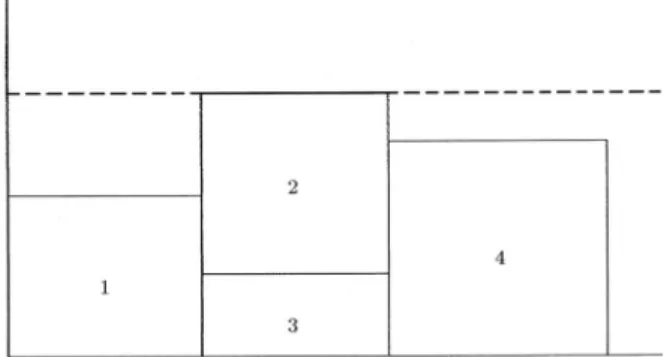
More than oneI may give the same schedule, i.e.,
the relation is one to many. For example, consider a single resource project with 4 real activities, whose activity on the node network is as shown in Figure 1.
Now, consider two chromosomes (012345)
and (013245). The schedules (phenotypes) of
these two genotypes are the same, as shown in Figure 2. Nodes 0 and 5 are dummies and not shown.
Generating Chromosomes and Setting Their
Resource Levels
Generating Chromosomes
For generating a chromosome I = (jI 0
jIn +1), at
the stage of determination of jIa, when jI 0
jIa ;1
are known, let Eligible Activity Set (EAS) be the set EAS=fujPu fjI
0 jIa
;1
gg and N(EAS) be the
number of activities in EAS. Then, the following two steps 3] are used:
1. Initial step: jI
0 = 0, EAS=
fujPu = f0ggN = N(EAS), a= 1,
2. Main step: If N = 0, stop. Otherwise, select one
Figure1. Activity on the nodes network.
Figure2. Resulted schedule from two dierent
of the activities from EAS and let it be activityi.
Set jIa =i and EAS= fuju2= fjI 0
jIaggPu fjI
0
jIaggN = N(EAS), a = a+ 1 and then
repeat the main step.
For selecting an activity from EAS, two methods are used, whose performances are compared later on. The rst method, which is suggested in 3], uses the ecient priority rule of minimum Latest Finish Time (LFT) to derive the probabilities of selecting activities from EAS. This method is referred to as RLFT. In RLFT, a probability for selecting each activity from EAS is assigned, proportional to the inverse value of the Latest Finish Time of that activity. The second method is suggested by Shadrokh and Kianfar 5], which is called WS. This method assigns the proba-bilities for selection of activities from EAS, such that chromosomes have more tendencies to appear with equal chance. It is shown that random selection of activities from EAS does not give an equal selection chance to all activity lists, i.e. chromosomes. Having the same chance for each chromosome to appear in the chromosome generating process gives an opportunity for the genetic algorithm to guide its population to the promising areas of later generations.
To dene WS, the following denitions are used: On an activity on the node network of a project, node j is reachable by node i 10], if there is at least
one directed path with origin i and terminus j. Let
the set of reachable nodes by node i be R Ni and
the number of elements of this set be N(R Ni). The
rightmost place on the activity list, where an activity,
i, could be placed, is n + 2;N(R Ni). Then, for
an activity, i, the bigger the value of N(R Ni), the
closer it would be to the left of the activity list and, hence, the number of location choices for this activity would be smaller. Noting this property, WS employs a simple heuristic for selecting activities from EAS, which gives each activity of EAS the chance of being selected proportional to its number of elements in the set of reachable nodes.
Setting Resource Levels
Each resource capacity should be determined, for each chromosome I. For this purpose, the Akpan
algo-rithm 6] was modied such that it would be applicable for RIPT.
Let TUkk 2 K = f1g be the total
amount of usage of resource k, which is equal for
all chromosomes and can be calculated as TUk = P
i=1n
rikDi. Also, let RES be a set containing
all resources. At this stage, RES = K. The resource
capacities for chromosomeI are determined using the
following steps:
Step 1 For chromosome I, schedule activities at the
earliest possible time, regardless of any re-source restriction
Step 2 Let all resource capacities be at their minimum possible levels. The minimum possible level for resourcek is the maximum level of resourcek
used in the earliest start time schedule along the time axis. Calculate the current untness value, UFcu, of this schedule, according to the
previous section
Step 3 Reduce one unit from the capacity of the resource that has a minimum value of
TUk=(Sn +1
Rk) 6], k 2 RES. In other
words, if mink2RES(
TUk=(Sn +1
Rk)) = TUv=(Sn
+1
Rv), reduce one unit from
re-source capacityv
Step 4 Consider the above values of the resource capacities as xed. Using SSS on chromosome
I, nd the start time of the activities. Let S
1
Sn
+1 be the calculated start times.
Calculate the untness value for this new schedule, UFnew
Step 5 If UFnew
> UFcu, delete resource v from set
RES and add one unit to its capacity. If set RES is empty, stop, the current resource capacities and the current untness value, UFcu, belong to chromosome I and one also
has its phenotype otherwise, go to Step 3. If UFnew
UFcu, let UFcu = UF
new and go to
Step 6 Step 6 IfSn
+1 >Sn
+1, set RES =
Kand go to Step 3.
Crossover
Here, two crossovers, i.e. one-point crossover 3] and two-point crossover 5], are considered and discussed below.
One-Point Crossover
Let Pa 1 = (
j 1 0
j 1
n+1) and Pa
2 = ( j
2 0
j 2
n+1)
be a pair of parents selected for crossover. Select integer numberrrandomly from the interval 1,n]. Two
children, CH1and CH2, are dened from this crossover,
whose activity list is (j 1 0 j 1 r;1 j 1
rj 1
n+1) for
CH1 and ( j 2 0 j 2 r;1 j 2
rj 2
n+1) for CH
2, where j
1 0
j 1
r;1 are j
1 0
j 1
r;1, arranged in the order
they are in Pa 2 and j 2 0 j 2
r;1 are j
2 0
j 2
r;1,
arranged in the order they are in Pa
1. For
example, if n = 5r = 4(j 1 0
j 1 6) =
(0153426) and (j 2 0
j 2 6) = (0
521436),
then (j 1 0 j 1 1 j 1 2 j 1 3 j 1 4 j 1 5 j 1
6) = (0
513426) and
(j 2 0 j 2 1 j 2 2 j 2 3 j 2 4 j 2 5 j 2 6) = (0
152436). Resource
capacities and untness values for children are deter-mined as explained previously.
Two-Point Crossover
Again, let Pa
1 = (
j 1 0
j 1
n+1) and Pa
2 = (
j 2 0
j 2
n+1) be a pair of parents.
Two integer random numbers, r 1 and r 2 r 1 < r 2,
are generated from the interval 1,n]. Two children,
CH1 and CH2, which result from this crossover, are
(j 1 0 j 1 r1 ;1 j 1 r1 j 1 r2 j 1 r2 +1 j 1
n+1) for CH 1
and (j 2 0 j 2 r1;1 j 2 r1 j 2 r2 j 2 r2+1 j 2
n+1) for
CH2, where j
1 0
j 1
r1;1 are j 1 0 j 1 r1
;1, arranged
according to the order they appear in Pa 2 and j 1 r2+1 j 1
n+1 are j 1 r2 +1 j 1
n+1, again, arranged
according to the order they are shown in Pa 2. The
denitions ofj 2
i's are similar.
For instance, consider two parents (j 1 0
, j
1
10) = (0
21573684910) and (j 2 0
j 2 10) =
(046825713910) and two integers r 1 = 4
andr
2 = 6, then, ( j 1 0 j 1 1 j 1 2 j 1 3 j 1 4 j 1 5 j 1 6 j 1 7 j 1 8 j 1 9 j 1 10)
= (025173648910) and (j 2 0 j 2 1 j 2 2 j 2 3 j 2 4 j 2 5 j 2 6 j 2 7 j 2 8 j 2 9 j 2 10) = (0
68425713910).
Because of the existence of precedence relations and the fact that two dierent chromosomes could have the same phenotypes, when the number of activities is not big enough (i.e., less than 30 activities), the two-point crossover usually will not give a new schedule. In such cases, even if a new child is produced, it is usually very similar to one of the parents and, therefore, it would be better to use a one-point crossover. On the other hand, if the number of activities are not small (more than 100), the one point method leads to children that may be very dierent from their parents and are similar to cases when a chromosome is produced randomly. Here, for saving the characteristics of the parents and for avoiding randomness behavior, it is better to use the two-point crossover.
Mutation
Let I = (jI 0
jIn
+1) be the chromosome that is
selected for mutation. An integer random number,a, is
generated from the interval 1,n]. Let activityjIb be the
last predecessor of activityjIa and activity jIc the rst
successor ofjIain chromosomeI. Then, another integer
random number, d, is generated from the interval
b+1c;1]. Ifd<a, then chromosomeI is replaced by
(jI 0
jId ;1
jIajIdjIa ;1
jIa +1
jIn
+1), but, if d>a, it would be replaced by (jI
0 jIa ;1 jIa +1 jId ;1 jIajId
+1 jIn
+1). The mutated chromosome
replacesI with a probability proportional to its
unt-ness. The process is the same as that of immigration, explained previously.
For example, consider chromosome (015372
4681191012). If a = 6 and activities 1 and
3 are the predecessors of 4 and 10 and 11 are its successors, a random number from 4 to 8 is
pro-duced. If d = 4 the mutated chromosome will be
(0153472681191012).
TESTING THE ALGORITHM
There is a dearth of published research on the Re-source Investment Problem, RIP. This is especially true about RIP benchmark problems with a known optimal solution. In particular, no algorithm has been presented to nd the optimal solution of RIPT. For adjusting the parameters of NGA, one needs to solve RIPT problems. Except for the 90 problems on RIP solved by Mohring 2], no other published set could be found. Shadrokh and Kianfar 5], show that this set of problems is simple and is not suitable for this purpose. The enumeration procedure was used on the resource capacities, together with the branch-and-bound procedure of Demeulemeester and Herroelen 11] and more than 700 problems were solved. ProGen software 8] was used to generate these problems. The enumeration procedure is as follows.
In solving each problem, the decision variables are the resource capacity and activity start times. Given a set of resource capacities, the value of the RIPT objective function is minimized by minimiz-ing Sn
+1. Therefore, the Single Mode Resource
Constrained Project Scheduling Problem (SMRCPSP) algorithms 11] can be used to nd the minimum objective function value of the RIPT, when resource capacities are set. Using this fact, RIPT can be solved by enumerating all possible combinations of resource capacities. It would be enough to consider all combinations of resource capacities between a lower bound, Rk, and an upper bound, Rk. For RIPT,Rks
(k = 1) cannot be less than maxi =1n
frikg
and, hence, Rk = maxi =1n
frikg. For RIP, Rks
(k = 1) cannot be less than maxi =1n
frikg
or less thanPn
i=1(
rikDi)=T, hence: Rk = maxf
n
X
i=1
(rikDi)=T max
i=1n frikgg:
The available capacity of resource k in the earliest
start time schedule is considered forRk(k= 1).
Problems with 10, 14 and 20 activities were generated, solved and used for this analysis.
The 480 instances presented in 12] were also used, which can be found in the project scheduling problem library PSBLIB 13], as will be explained in the next sections. Also, various sensitivity analyses of computa-tional performance on some problem parameters have been presented.
All the computations were performed on an IBM-compatible PC with a Pentium III, 1 GHz CPU speed and 256 MB RAM memory, under Windows 2000 as the operating system. Also, all procedures were coded in
ANSI C and compiled with the Microsoft Visual C++ 6.0 compiler.
ProGen Instances with 20 Non-Dummy
Activities
20 instances, with 20 non-dummy activities and 4 resources, were generated with ProGen software 8]. The user can set a number of parameters in this program. Three important parameters that can be set are as follows:
1. NC (Network Complexity): The average number of non-redundant arcs per node, including the dummy activities
2. RF (Resource Factor): The average percentage of dierent resource types for which each non-dummy activity has a non-zero resource demand
3. RS (Resource Strength): It shows the availability amount of resources. An RS value of zero denes the capacity of the resource to be no more than the maximum demand over the set of all activities, while an RS value of 1 denes the capacity of each resource to be equal to the demand imposed by the earliest start time schedule.
For these problems, activity duration and re-source requirements for each of the 4 rere-source types are integer values within the range 1,10], according to a discrete uniform distribution. The project net-works have three (non-dummy) start activities and three (non-dummy) nish activities. The Network Complexity, NC, is set at 1.5 and the Resource Factor, RF and Resource Strength, RS, are set to 1 and 0.2, respectively (for more details see 8]). The maximum number of predecessors/successors is three. The orig-inal resource availabilities of SMRCPSPs, which are generated by ProGen, are used as the unit costs of the corresponding resource types. Also, the tardiness cost,
Cd, is considered as 1/8 of the sum of the unit cost of
the resources. If the selected parameter is too high, the solution of the RIPT comes close to that of RIP and, if it is too low, the resource availabilities tend toward their lower bounds and tardiness becomes too long.
To get a RIPT instance, one additionally needs the due date, T. In this study, T =
EFT was
set where EFT is the earliest nish time of the project having innite resource capacities and 2 f1:01:11:21:31:41:5g. Using the enumeration
pro-cedure, the optimal solution and the value of the objective function were obtained for these 120 prob-lems. Having the optimal solutions, one can adjust the parameters of the genetic algorithm. The following selections were used for the parameter values: POP
2 f1020gPmu 2 f0:10:2g and P cr
2 f0:51g. A
complete factorial design of the above parameters is
considered, so that a total number of 222120 = 960
problems have been tested using NGA for RIPT. For adjusting the parameters, POP, Pmu and P
cr, SSS
and WS were employed for selecting activities from EAS. Then, average and maximum percent deviation from the optimal solution and the percentage of the problems that reached optimality were calculated. The average number of generations for 2 seconds computing time was 121.13. For the statistical analysis of the results on the percent deviation from the optimal solu-tion, knowledge of its distribution function is needed. Although this random variable is not necessarily nor-mally distributed, since the average percent deviation of 120 problems is being studied based on the central limit theorem, one can safely assume that this average percentage is normally distributed. This assumption was supported using the goodness of t test. In the sta-tistical analysis, in order to nd good combinations of the NGA parameters, multi factor analysis of variance was employed. Analysis of variance showed that all of the above factors are statistically signicant. Using a Duncan multiple range test, the following rankings were observed: for POP 1020, for Pmu0:10:2
and for P cr1
0:5, where \" denotes better and
\" denotes signicantly better. Table 1 shows the
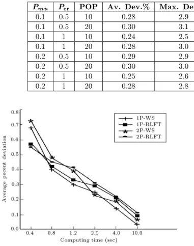
combinations of the parameter values and their results with 2 seconds computing time. Without going into detail, it is interesting to note that if these problems were considered as RIP, the percentage of problems to reach optimality would be between 88 and 95.5. The last column of Table 1 shows the percentage of problems that reached optimality when considered as RIP.
For testing the eects of crossover operator, se-lection method from EAS and computing time limit, two crossover operators were considered, i.e., one-point crossover (1P), two-one-point crossover (2P) and two selection methods, i.e. WS and RLFT.
For this test, POP = 10,Pmu= 0:1 andP cr= 1
were considered. Again, a complete factorial design was employed and 22120 = 480 problems were evaluated.
Average percent deviation from the optimal solution was calculated for a 0.4, 0.8, 1.2, 2, 4 and 10 second computing time limit. Figure 3 shows the results: The X-axis shows the computation times and the Y-axis shows the average percent deviations from the optimal solution. A multi factor analysis of variance was conducted. For all selected time limits and with a condence level of less than 1%, there was a statistically signicant dierence between the crossover operators and, also, between the selection methods.
Figure 3 shows that RLFT is better for time limits less than 1.2 seconds and WS outperforms the others for time limits exceeding 1.2 seconds. This was expected, since WS tries to assign uniform probabilities to all possible activity lists. This property gives the
Table1. Combinations of parameter values. Pmu P
cr
POP Av. Dev.% Max. Dev.% RIPT Optimal% RIP Optimal%
0.1 0.5 10 0.28 2.9 49 92.2
0.1 0.5 20 0.30 3.1 48.3 88.2
0.1 1 10 0.24 2.5 54.3 95.5
0.1 1 20 0.28 3.0 51.1 90.1
0.2 0.5 10 0.29 2.9 49.2 89.3
0.2 0.5 20 0.30 3.0 48.5 89
0.2 1 10 0.25 2.6 49.2 91.1
0.2 1 20 0.28 2.8 47.8 90.2
Figure3. Average percent deviation from optimal
solution for four combinations of crossover operators and selection methods from EAS for RIPT.
NGA a chance to nd the promising areas of the feasible solutions, provided it has enough time to reach them.
On the other hand, RLFT gives a higher chance to those activity lists that seem promising and, hence, it is expected that RLFT will perform better for shorter time limits. However, the optimal solution may not be among the activity lists that RLFT selects with a higher probability.
The above problems were also tested when the tardiness penalty is very large. In this case, in fact, one has RIP. The results are shown in Figure 4. Multiple factor analysis of variance showed a statistically sig-nicant dierence between the selection methods from EAS with a condence level of less than 1% for all time limits, but no signicant dierence was observed between dierent crossover operators for time limits greater than 0.8 seconds.
ProGen Instances with 10 and 14 Non-Dummy
Activities
For more analysis of the performance of the NGA, 20 instances with 10 activities and 20 instances with 14 activities were generated and tested, each with 4
Figure4. Average percent deviation from optimal
solution for four combinations of crossover operators and selection methods from EAS for RIP.
resources using ProGen, with the same parameters used for the 20 activity problems mentioned previously.
Here, again, one set T =
EFT,
2
f1:01:11:21:31:41:5g. Therefore 2
206 = 240
problems were generated and solved, both as RIP and RIPT (480 problems altogether), using the enumera-tion procedure described before. These problems were given to the NGA with the following parameters: POP =10,Pmu= 0:1 andP
cr= 1.
Tables 2 and 3 show the results of this test for RIPT and RIP, respectively, considering a computing time limit of 0.4 seconds. These tables also contain the results of the 20 activity problems mentioned previously.
Table2. Results of NGA on RIPT with 10, 14 and 20
problems within 0.4 seconds.
No. of
Activities
Av. Dev.
%
Max. Dev.
%
Optimal
%
10.00 0.04 0.25 50.50 14.00 0.05 0.29 43.03 20.00 0.55 3.95 38.21
Table3. Results of NGA on RIP with 10, 14 and 20
problems within 0.4 seconds.
No. of
Activities
Av. Dev.
%
Max. Dev.
%
Optimal
%
10.00 0.00 0.00 100.00 14.00 0.04 3.98 97.80 20.00 0.63 7.20 69.70
ProGen Instances with 30 Non-Dummy
Activities
Drexl and Kimms 12] used mathematical program-ming to nd the lower bound, LB, and the upper
bound,UB, for RIP. They employed two mathematical
programming techniques, Lagrangian relaxation and Column generation, to construct two algorithms for nding these bounds. To measure the eectiveness of their algorithms, they used the two following measures of performance:
percentage of improvement of the upper bound =UB
0 ;UB UB
0
100
Percentage of improvement of the lower bound =LB;LB
0 LB
0
100
where UB
0 is the objective function value of the
problem, if one setsRks at their obvious upper bounds, Rks, andLB
0is the value of objective function, if one
sets Rks at their obvious lower bounds, Rks (Rks and Rks were given in previous sections).
The two algorithms were tested on 480 instances with 30 non-dummy activities and 4 resources from the project scheduling problem library PSBLIB 13]. The resource limits are ignored in their test, since the
resource limitation is irrelevant in RIP. For these prob-lems, the ProGen parameters were: NC2f1:51:82:1g
and RF2f0:250:50:751:0g. For each combination of
NC and RF, 40 instances exist in PSBLIB, which gives a total of 3440 = 480 instances. For each instance,
the value of the project due dateT, is considered asT =
EFT, where
2 f1:01:11:21:31:41:5g. This
gives a test bed of 6480 = 2880, RIP problems. Also,
a random number was chosen from the interval 1,10] as the unit resource cost for each resource 14]. For each investigated instance, the average percentage of improvement of the lower bound and the upper bound, using Lagrangian relaxation and column generation methods, is computed.
All these 2880 problems were given to the NGA with the following parameters: POP = 10Pmu =
0:1P cr= 1
2P and WS, with a computing time limit
of 2 seconds. The result of the NGA for each instance is the best feasible individual in the nal population and the untness value of this individual is an upper bound for the instance. The NGA algorithm does not produce a lower bound, therefore, to evaluate the performance of the NGA using the above problems, only the percentage improvement of the upper bound (100(
UB 0
; UB)=UB
0) is compared with that of
Drexl and Kimms 12]. Table 4 shows the percentage improvement of the upper bound using NGA.
The average number of generations for these problems was 102.82. The comparison of the entries in Table 4 with those of Drexl and Kimms 12] and, also, with SKGA shows that the NGA performs much better in nding upper bounds.
CONCLUSION
A new genetic algorithm is presented for solving the resource investment problem when tardiness is per-mitted with a penalty. This algorithm has many parameters. To adjust the parameters 120 RIPT
Table4. Average percent improvement of the upper bound using NGA.
n
= 30
1
1.1
1.2
1.3
1.4
1.5
RF = 0.25 34.60 40.56 42.46 43.36 43.86 44.12
NC = 1.5
RF = 0.5 32.25 41.54 46.60 50.36 53.56 55.84RF = 0.75 36.27 42.95 47.43 51.23 54.27 56.95 RF = 1 38.20 43.68 48.30 52.00 55.13 57.50 RF = 0.25 29.68 36.99 40.04 41.11 41.45 41.60
NC = 1.8
RF = 0.5 30.26 39.00 44.17 48.56 51.08 53.56RF = 0.75 33.53 39.79 44.51 48.09 51.07 53.78 RF = 1 29.69 37.36 42.05 46.40 49.83 52.52 RF = 0.25 24.79 34.70 38.30 38.92 39.18 39.40
NC = 2.1
RF = 0.5 27.88 36.66 42.49 46.75 49.79 52.52RF = 0.75 26.50 35.15 40.41 44.56 48.14 50.90 RF = 1 29.80 37.50 42.71 46.63 49.49 52.16
and 120 RIP were solved to optimality, each with 20 activities. These solved problems were also used in testing the computational performance of NGA. Additionally, for the computational performance test 240 RIPT and 240 RIP were also solved, with 10 and 14 activities to optimality. The NGA results on these problems, compared with SKGA results and their optimal solutions, were quite satisfactory.
In addition, Drexl and Kimms problems 12] were used for test purposes only, on the basis of the upper bound on the optimal value of the objective function. The performance of the NGA on these problems was also very good.
REFERENCES
1. Baker, K.,Introduction to Sequencing and Scheduling, John Wiley and Sons, Inc. (1974).
2. Mohring, R.H. \Minimizing costs of resource require-ments in project networks subject to a x completion time",Operations Research,32pp 89-120 (1984).
3. Hartmann, S. \A competitive genetic algorithm for resource-constrained project scheduling", Naval Re-search Logistics,45, pp 733-750 (1998).
4. Pritsker, A.A.B., Watters, L.J. and Wolfe, P.M. \Multi-project scheduling with limited resources",
Management Science,16, pp 93-108 (1969).
5. Shadrokh, S. and Kianfar, F. \A genetic algorithm for resource investment project scheduling problem, tardiness permitted with penalty", Industrial Engi-neering Department, Sharif University of Technology,
European Journal of Operational Research(in press).
6. Akpan, E.O.P. \Optimal resource determination for project scheduling",Production Planning and Control,
8(5), pp 462-468 (1997).
7. Kelley, J.E., Jr. \The critical path method: Re-sources planning and scheduling",Industrial Schedul-ing, Prentice-Hall, J.F. Muth and G.L. Thompson, Eds., New Jersey, pp 347-365 (1963).
8. Kolish, R. \Serial and parallel resource constrained project scheduling methods revisited: Theory and computation", European Journal of Operational Re-search,90, pp 320-333 (1996).
9. Kolisch, R. and Hartmann, S. \Heuristic algorithms for the resource constrained project scheduling problem: Classication and computational analysis", Project Scheduling, J. Weglarz, Ed. (1999).
10. Schwindt, C. \Generation of resource constrained scheduling problems with minimal and maximal time lags", Report WIOR-489, Universitat Karlsruhe (1996).
11. Demeulemeester, E. and Herroelen, W. \A branch-and-bound procedure for the multiple resource-constrained project scheduling problem",Management Science,38, pp 1803-1818 (1992).
12. Drexl, A. and Kimms, A. \Optimization guided lower & upper bounds for the resource investment problem",
Journal of the Operational Research Society, 52, pp
340-351 (2001).
13. Kolisch, R. and Sprecher, A. \PSBLIB- A project scheduling problem library",European Journal of Op-erational Research,96, pp 205-216 (1997).