A bi-objective model to optimize reliability and cost of k-out-of-n series-parallel systems with tri-state components

Sharif University of Technology

Transactions E: Industrial Engineering www.scientiairanica.com

A bi-objective model to optimize reliability and cost of

k-out-of-n series-parallel systems with tri-state

components

P. Pourkarim Guilani

_{, A. Zaretalab}

_{, S.T.A. Niaki}

_{and P. Pourkarim Guilani}

b. Department of Industrial Engineering, Amirkabir University of Technology, 424 Hafez Ave., Tehran, Iran. c. Department of Industrial Engineering, Sharif University of Technology, Tehran, P.O. Box 11155-9414, Iran. Received 27 April 2016; received in revised form 15 January 2017; accepted 28 January 2017

KEYWORDS Reliability; Redundancy allocation problem; Tri-state components; Bi-objective

optimization; SPEA-II.

Abstract. Redundancy Allocation Problem (RAP) is one way to increase system reliability. In most of the models developed so far for the RAP, system components are considered to have a binary state consisting of \working perfect" or \completely failed". However, to suit the real-world applications, this assumption has been relaxed in this paper, such that components can have three states. Moreover, a Bi-Objective RAP (BORAP) is modeled for a system with serial subsystems, in which non-repairable tri-state components of each subsystem are congured in parallel and the subsystem works under k-out-of-n policy. Furthermore, to enhance system reliability, technical and organizational activities that can aect failure rates of the components, and hence can improve the system performance are also taken into account. The aim is to nd the optimum number of redundant components in each subsystem, such that the system reliability is maximized while the cost is minimized within some real-world constraints. In order to solve the complicated NP-hard problem at hand, the multi-objective Strength Pareto Evolutionary Algorithm (SPEA-II) is employed. As there is no benchmark available, the Non-dominated Sorting Genetic Algorithm (NSGA-II) is used to validate the results obtained. Finally, the performances of the algorithms are analyzed using 20 test problems.

© 2017 Sharif University of Technology. All rights reserved.

1. Introduction

Growing customer demands and increased production rates to satisfy the demands have made reliability engineers think of ways to enhance the reliability of production systems in their designs. One way to increase system reliability is the so-called redundancy allocation optimization. The Redundancy Allocation

*. Corresponding author.

E-mail addresses: pedram [email protected] (P. Pourkarim Guilani); arash [email protected] (A. Zaretalab); [email protected] (S.T.A. Niaki); pardis [email protected] (P. Pourkarim Guilani)

Problem (RAP) is a complex combinational optimiza-tion problem in which the goal is to determine the optimal combination of the number of components of a system in order to maximize its reliability under some constraints. This problem has many applications in industries such as electronic systems, power stations, production systems, etc.

Based on the classical standpoint, system compo-nents in reliability models are considered to operate in two working conditions of \perfect" and \failed", based on which many RAP models have been proposed in the literature. Fye et al. [1] were the rst to model the RAP using an active strategy. The objective function of their model maximized system reliability subject to

weight and cost constraints. They employed dynamic programming to solve the problem. Nakagawa and Miyazaki [2] solved 33 problems based on Fye et al.'s model [1]. In these problems, the upper limit on the system weight was ranging from 159 to 191. They used an exact method, called surrogate constraint, to solve the problems, and showed that this approach would perform better than the dynamic programming method in problems with multiple constraints. Moreover, Buln and Liu [3] utilized three methods to solve these 33 problems. Two of them were exact methods based on branch and bound, and the third was a heuristic approach.

Misra and Sharma [4] considered RAP for a series-parallel conguration with subsystems that work under k-out-of-n policy. In their models, the redundancy strategy was active, and similar components, each with two sates, could be allocated to each subsystem. They solved the problem using zero-one programming. Bai et al. [5] developed a RAP model for a k-out-of-n subsystem under the Common-Cause Failures (CCF). Pham [6] proposed a RAP model for a system with only one k-out-of-n subsystem under the active strategy. The objective function of his proposed model was to minimize the total cost of the system. She and Pecht [7] derived a closed-form formula to calculate the reliability of k-out-of-n subsystem with warm-standby redundancy. Pham and Malon [8] presented a model for the RAP of a k-out-of-n subsystem under active strategy with similar multiple failure-state com-ponents. Coit and Smith [9] proposed a new model with a mix of components (RAPMC) and active strategy for series-parallel systems with k-out-of-n subsystems. Assuming that there would be uncertainty in com-ponent reliability, Coit and Smith [10] investigated the RAP of series-parallel systems with k-out-of-n subsystems consisting of similar components under active strategy. Moreover, Coit and Liu [11] proposed a RAP model with CCF and k-out-of-n strategy, in which both the active and standby strategies were used simultaneously. In order to solve the problem, they used a zero-one integer programming. Taking into consideration the active and cold-standby strategies, Coit [12] developed a new RAP model and solved it using integer programming. Moreover, Tian et al. [13] presented a joint redundancy-reliability optimization method in order to solve series-parallel RAP. They displayed that technical and organizational activities are eective approaches to improve system reliability, where failure and repair rates of components could be improved by these activities.

Since the time Chern [14] proved that RAP belongs to the class of NP-hard problems, several heuristics and metaheuristics have been proposed in the literature to solve various RAPs. Ida et al. [15] and Yokota et al. [16] were the rst to present a simple

Ge-netic Algorithm (GA) to solve RAP for series-parallel system with multiple failure-state components. In order to generate and select feasible solutions, Coit and Smith [17] introduced a performance penalty function to encourage algorithm to search the boundaries be-tween feasible and near-feasible regions. Furthermore, Coit [18] solved the problems in [1] under the cold-standby redundancy strategy. Tavakkoli-Moghaddam et al. [19] developed a GA to solve the problems solved in [12]. An important characteristic of their GA was the type of chromosome and the crossover and mutation operators. Safaei et al. [20] studied the performance of a Particle Swarm Optimization (PSO) algorithm, named Annealing-based PSO (APSO), to solve RAP with multiple component choices. Moreover, Chambari et al. [21] solved the problems in [12] using an ecient Simulated Annealing (SA) and compared the results with the ones obtained in [19]. Teimouri et al. [22] pre-sented an ecient Memory-Based Electromagnetism-like Mechanism (MBEM) to solve the RAP. They used a memory matrix in the local search procedure to separate positive variations from negative ones in order to nd better solutions. Recently, Pourkarim Guilani et al. [23] have worked on a RAP with in-creasing failure rates of system components under the Weibull distribution. They employed a simulation-based optimization approach to estimate the system reliability function and utilized a GA to solve their problem.

While the aforementioned studies considered sys-tem components to work in the two states of \working perfect" or \completely failed", to suit real-world applications, this assumption will be relaxed in this paper, such that the components can perform at any performance rate between 0% and 100%, each with a certain probability. To name a few works in this regard, Levitin et al. [24] oered a model to determine optimal versions of components and their redundancy in multi-state series-parallel systems. Besides, while Ramirez-Marquez and Coit [25] utilized a heuristic method to solve a multi-state RAP, Tian and Zuo [26] proposed a new solution method based on physical programming. Note that the number of possible states in a system with multi-state components increases rapidly when the number of subsystems becomes larger, and hence computational complexity gets high so that system reliability determination of Multi-State Systems (MSS) is extremely hard using mathematical relations. In this situation, the Universal Generating Function (UGF), rst proposed by Ushakov [27], is usually used. Levitin and Lisnianski [28] employed the UGF and proposed a method to solve a multi-state system reliability optimization problem. The technique presented in their paper combines a UGF method used for fast reliability evaluation of MSS and a GA used as an optimization engine. Lisnianski and Levitin [29]

studied UGF applications in reliability evaluation of some MSSs with series, parallel, and series-parallel subsystems. One diculty in the application of the UGF method to calculate reliability and availability of MSSs is the CPU time, required when the number of components in the system increases. To cope with this problem, Li and Zuo [30] presented another useful method, called recursive algorithm, which evaluates reliability and availability of MSSs in short CPU time. Besides, Pourkarim Guilani et al. [31] presented another ecient method in order to calculate the reliability of non-reparable thri-state systems using a Markov model. They demonstrated that with an appropriate denition of the states, the reliability of thri-state systems can be calculated in even shorter CPU time compared to the recursive algorithms; thus, it can be utilized to evaluate the reliability of large-scale problems. Furthermore, Pourkarim Guilani et al. [32] provided a RAP model to optimize reliability of series-parallel systems with thri-state components based on [31]. In order to validate the results obtained by a GA solution method, they proposed an exact enumeration method.

RAP, with multiple objectives, due to its real-world applications, has recently received much at-tention in the literature. In Multi-Objective RAP (MORAP), in addition to reliability optimization, some other objective functions, such as cost and weight minimizations, are involved. In this regard, Cham-bari et al. [33] presented a bi-objective model for RAP in series-parallel systems under some assump-tions such as repairable, cold standby, and active strategy. They solved the problem using both Non-dominated Sorting GA (NSGA-II) and Multi-Objective Particle Swarm Optimization (MOPSO) algorithms. Khalili Damghani and Amiri [34] solved a binary-state MORAP using an epsilon-constraint programming, multi-start partial bound numeration algorithm, and Data Envelopment Analysis (DEA). Safari [35] pre-sented a MORAP for a series-parallel system by con-sidering non-repairable components and independent failures. He solved the problem using NSGA-II. Khalili Damghani et al. [36] presented a Decision Support System (DSS) to solve MORAPs, where a reduced-dimension multiple objective optimization problem was used.

In this paper, we intend to present a bi-objective model to optimize reliability and cost of series-parallel system with k-out-of-n subsystems. The important assumption in this research is that the components of the subsystems can have three performance rates. The reason for investigating thri-state systems is their wide applicabilities to real-world system reliability problems. Although thri-state systems belong to the larger class of multi-state systems, many real-world systems, especially mechanical systems, work with

components with three states: fully-working, semi-working, and failed [31]. In addition, the impact of technical and organizational activities on system reliability is considered. Due to NP-hardness of the problem, the multi-objective Strength Pareto Evolu-tionary Algorithm (SPEA-II) is employed to solve it. Besides, as there is no benchmark available in the literature, a NSGA-II algorithm is used to validate the results obtained. A summary of the literature review is provides in Table 1.

The organization of the rest of the paper is as follows. The problem is dened in Section 2. In Section 3, the parameters, variables, and model of the problem are presented. Solution methods are described in Section 4. Numerical examples are given in Section 5 to not only demonstrate the applicability of the proposed methodology, but also to validate the results obtained using SPEA-II. Finally, in the last section, we will present conclusion and directions for future research.

2. Problem denition

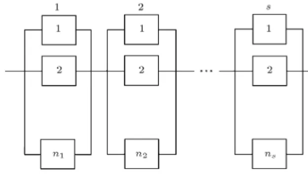
Consider a system consisting of s sub-systems in series. A sub-system has ni components in parallel. It is

assumed that each component has three states of fully-working (100% performance), semi-working (50% performance), and not working or failed (0% perfor-mance) [31]. The system structure is demonstrated in Figure 1. Moreover, as the subsystems are congured in series, failure of a subsystem causes the system to fail. The components are non-repairable with Constant Failure Rates (CFR). The components of ith sub-system, i = 1; 2; ; s, have three dierent failure rates as follows:

i1 Moving from 100% to 50% working;

i2 Moving from 100% to 0% working;

i3 Moving from 50% to 0% working.

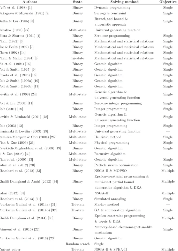
Similar to Pourkarim Guilani et al. [31], the notation (w; m) is used to represent a subsystem with w fully-working and m semi-fully-working components. Then, the number of states associated with a (w; m) subsystem with performance point of k, k = 0; 1; 2; ; 2ni

Table 1. A summary of relevant literature.

Authors State Solving method Objective

Fye et al. (1968) [1] Binary Dynamic programming Single

Nakagawa & Miyazaki (1981) [2] Binary Surrogate constraint Single Buln & Liu (1985) [3] Binary Branch and bound &

a heuristic approach Single

Ushakov (1986) [27] Multi-state Universal generating function | Misra & Sharma (1991) [4] Binary Zero-one programming Single Pham (1992) [6] Binary Mathematical and statistical relations Single She & Pecht (1992) [7] Binary Mathematical and statistical relations Single Chern (1992) [14] Binary Mathematical and statistical relations Single Pham & Malon (1994) [8] tri-state Mathematical and statistical relations Single

Ida et al. (1994) [15] Binary Genetic algorithm Single

Coit & Smith (1995) [9] Binary Genetic algorithm Single

Yokota et al. (1995) [16] Binary Genetic algorithm Single

Coit & Smith (1996a) [10] Binary Genetic algorithm Single

Coit & Smith (1996b) [17] Binary Genetic algorithm Single

Levitin et al. (1998) [24] Multi-state Genetic algorithm &

universal generating function Single Coit & Liu (2000) [11] Binary Zero-one integer programming Single

Coit (2001) [18] Binary Integer programming Single

Levitin & Lisnianski (2001) [28] Multi-state Genetic algorithm &

universal generating function Single

Coit (2003) [12] Binary Integer programming Single

Lisnianski & Levitin (2003) [29] Multi-state Universal generating function | Ramirez-Marquez & Coit (2004) [25] Multi-state Heuristic method Single Tian & Zuo (2006) [26] Multi-state Physical programming Single Tavakkoli-Moghaddam et al. (2008) [19] Binary Genetic algorithm Single

Li & Zuo (2008) [30] Multi-state Recursive algorithm |

Tian et al. (2009) [13] Multi-state Genetic algorithm Single

Safaei et al. (2012) [20] Binary Particle swarm optimization Single

Chambari et al. (2012) [33] Binary NSGA-II & MOPSO Multiple

Khalili Damghani & Amiri (2012) [34] Binary

Epsilon-constraint programming & multi-start partial bound

numeration algorithm & DEA

Multiple

Safari (2012) [35] Binary NSGA-II Multiple

Chambari et al. (2013) [21] Binary Simulated annealing Single

Pourkarim Guilani et al. (2014a) [31] Tri-state Markov method | Pourkarim Guilani et al. (2014b) [32] Tri-state GA & enumeration algorithm Single Khalili Damghani et al. (2014) [36] Binary Epsilon-constraint programming

& topsis & DEA Multiple Teimouri et al. (2016) [22] Binary Memory-based electromagnetism-like

mechanism Single

Pourkarim Guilani et al. (2016) [23] Binary Genetic algorithm Random search Single

Figure 2. State space diagram of a subsystem [31].

1; 2ni, is obtained by:

2w + m = k; k = 0; 1; 2; ; 2ni 1; 2ni;

w + m ni: (1)

Besides Pourkarim Guilani et al. [31] showed that based on the state space diagram of a subsystem f(w; m); w; m nig denoted by f(w; m); w; m nig

shown in Figure 2, the set of dierential equation (Eq. (2)) is obtained and solved using the matrix model in order to calculate the probability of the states.

8 > > > > > > > > > > > < > > > > > > > > > > > :

P0

(ni;0)(t) + (nii1+ nii2)P(ni;0)(t) = 0;

w = ni; m = 0;

P0

(w;m)(t) + (wi1+ wi2+ mi3)P(w;m)(t)

= (w + 1)i1P(w+1;m 1)(t)

+ (w + 1)i2P(w+1;m)(t)

+ (m + 1)i3P(w;m+1)(t)

; w; m < n

(2)

Then, the reliability of sub-system i is: Ri(t) =

X

(w;m)2R[W;m] (0;0)

P(w;m)(t): (3)

Based on k-out-of-n design, a subsystem works if at least k out of its n parallel components is fully working. However, this denition cannot be used for subsystems with tri-state components. Here, based on the point system dened earlier, we assume that each subsystem works successfully if and only if its assigned point is at least ki, (0 < ki < 2ni). Besides,

as mentioned previously, the points assigned to fully-working and semi-fully-working components are considered 2 and 1, respectively. As a result, the point the subsystem (w; m) receives is 2w + m. In this case, the reliability of subsystem i with tri-state components that works under ki-out-of-ni will be:

Ri(t) =

X

(w;m)2R[W;m] 8[2w+m<ki]

P(w;m)(t): (4)

In the next subsection, a numerical example is given to illustrate the proposal.

2.1. A numerical example

Let a sub-system have three identical tri-state compo-nents. Then, its number of states is obtained by:

2w + m = k; k = 0; 1; 2; ; 6;

w + m 3: (5)

Eq. (5) can be decomposed into seven equations as follows:

k = 6 )

2w + m = 6 w + m 3

) (w; m) = f(3; 0)g; k = 5 )

2w + m = 5 w + m 3

) (w; m) = f(2; 1)g; k = 4)

2w + m = 4 w + m 3

) (w; m) = f(2; 0); (1; 2)g; k = 3)

2w + m = 3 w + m 3

Figure 3. State space diagram of the example [31].

Table 2. Matrix representation of the example based on space state diagram. n = 3 (3,0) (2,1) (2,0) (1,2) (1,1) (0,3) (1,0) (0,2) (0,1) (0,0)

(3,0) 0 31 32 0 0 0 0 0 0 0

(2,1) 0 0 3 21 22 0 0 0 0 0

(2,0) 0 0 0 0 21 0 22 0 0 0

(1,2) 0 0 0 0 23 1 0 2 0 0

(1,1) 0 0 0 0 0 0 3 1 2 0

(0,3) 0 0 0 0 0 0 0 33 0 0

(1,0) 0 0 0 0 0 0 0 0 1 2

(0,2) 0 0 0 0 0 0 0 0 23 0

(0,1) 0 0 0 0 0 0 0 0 0 3

(0,0) 0 0 0 0 0 0 0 0 0 0

k = 2)

2w + m = 2 w + m 3

) (w; m) = f(1; 0); (0; 2)g; k = 1 )

2w + m = 1 w + m 3

) (w; m) = f(0; 1)g; k = 0 )

2w + m = 0 w + m 3

) (w; m) = f(0; 0)g: (6) Therefore, all of the possible states of this subsystem are:

R(w;m)= f(0; 0); (0; 1); (0; 2); (0; 3); (1; 0); (1; 1);

(1; 2); (2; 0); (2; 1); (3; 0)g: (7) Moreover, in 1-out-of-n case, the subsystem continues working in all states except (0; 0), whereas in k-out-of-n case with k = 3, the subsystem cok-out-of-ntik-out-of-nues workik-out-of-ng ik-out-of-n all of the following states:

R(w;m)k-out-of-n=f(0; 3);(1; 1);(1; 2);(2; 0);(2; 1);(3; 0)g:

(8)

The state space diagram of this subsystem is shown in Figure 3 with a matrix model given in Table 2. 2.2. Technical and organizational activities Technical and organizational activities involve sup-portive actions such as system monitoring, using specic maintenance programs, changing maintenance programs, etc. These activities are eective tools to improve failure and repair rates of the components that result in system reliability improvement. In general, activities that are performed at the component level are called technical and those performed at the subsystem level are organizational. Both of these activities try to improve availability of the system by inuencing transition rates in dierential equations. The dierence between these two types of activities is that technical activities have impact only on special components of a subsystem and their cost depends on the number of aected components, whereas organizational activities aect the whole components of subsystems and their cost is independent of the number of components.

Let be the eect of technical activities on a component and tkh be a binary variable that takes 1 if the activity is performed, and zero otherwise. Then, Eq. (9) shows how a technical activity inuences failure rate () of a component:

0_{= tkh::: (9)}

In Eq. (9), the failure rate of a component is reduced from to 0 _{in order to enhance system}

reliabil-ity. Similar approach is taken to model the eect of organizational activities. In this paper, both of the above activities are considered to improve system reliability. Interested readers are referred to [13] for more details.

3. Mathematical formulation

In order to present the mathematical model of the problem at hand, the notations are rst introduced. 3.1. Nomenclature

The notations used to model the problem are dened as:

i Index of a subsystem, i = 1; 2; : : : ; s

s Number of sub-systems

ni Number of components in subsystem i,

ni= 1; 2; ; nmax

R System reliability

Ri(t) Reliability of ith subsystem at time t

ci Cost of a redundant component in

subsystem i

i Interconnection cost coecient for a

component in ith subsystem ki Minimum requirement point of ith

subsystem to work

K The vector of minimum requirement

points [k1; k2; ; ks]

ckhhi Variable cost of hth technical activity

on a component of ith subsystem h = 1; 2; ; Hi

ckohi Constant cost of hth technical activity

on a component of ith subsystem Hi Number of available technical activities

on components of ith subsystem ckfi Cost of fth organizational activity on

ith subsystem, f = 1; 2; ; Fi

Fi Number of available organizational

activities on ith subsystem ij jth type of failure rate for the

components of ith subsystem 0

ij Updated failure rate based on technical

and organizational activities

tkhhi A binary variable equals 1 if technical

activity type h is performed on a component of ith subsystem; zero otherwise

tkfi: A binary variable equals 1 if

organizational activity type f is performed on ith subsystem; zero otherwise

hij The eect of technical activity type

h on jth type of failure rate for the components of ith sub-system fij The eect of organizational activity

type h on jth type of failure rate for the components of ith sub-system 3.2. The model

The bi-objective optimization model of the redundancy allocation problem at hand is:

max : R =Ys

i=1

Ri(t); (10)

min : C =Xs

i=1

(

nici+ eni(i)

+

Hi

X

h=1

([ckhhi:ni+ ckohi]:tkhhi)

+

Fi

X

f=1

(ckfi tkfi)

)

; (11)

s.t.: 0

ij= ij tkhhi:ij:hij; 8 i; j; h; (12)

0

ij= ij tkfi:ij:fij; 8 i; f; j; (13)

K 2 [k1; k2; ; ks]; (14)

ni nmax; 8 i; (15)

ni 0; 8 i; (16)

tkhhi= 0; 1; 8 h; i; (17)

tkfi= 0; 1; 8 f; i: (18)

Eq. (10) is the rst objective function of the problem to maximize the system reliability. It is obtained by multiplication of the reliability of the serial subsystems (the relation between Ri(t) and ni was explained in

Section 2). Eq. (11) represents the second objective function to minimize the total cost including the cost to purchase the components, the interconnection cost modeled by an exponential distribution [37], the cost

of technical activities, and the cost of organizational activities. Eqs. (12) and (13) are constraints on technical and organizational activities, respectively. Relation (14) shows the number of minimum require-ment points for a subsystem to be in a working condition. These values are predetermined due to the need of each subsystem. Constraint (15) puts an upper bound on the number of components of the subsystems; Constraint (16) is a sign constraint; Eqs. (17) and (18) dene the binary variables used for either performing technical and organizational activities or not.

In the next section, a multi-objective Strength Pareto Evolutionary Algorithm (SPEA-II) is employed to solve the problem.

4. Solving methods

As mentioned, as RAP is classied as an NP-hard problem, exact methods are not suitable to solve it, especially for problems with relatively large sizes. The problem investigated here consists of two objectives: one being related to RAP and the other to the sys-tem cost. Thus, a population-based multi-objective evolutionary algorithm, called SPEA-II, is developed in this paper for a Pareto solution. Besides, as there is no benchmark available in the literature, an-other commonly used population-based multi-objective meta-heuristic, called NSGA-II, is utilized to validate the results obtained. Both algorithms are population-based that share similar structures. The chromosome of both algorithms is (1 s) vector n that contains the number of components used in dierent subsystems. This chromosome is shown in Figure 4. Besides, the answering structure that contains technical and orga-nizational activities is s (H + F ) matrix containing binary elements shown in Figure 5.

Figure 4. The chromosome structure of the algorithms.

Figure 5. The answering structure of technical and organizational activities.

For instance, consider a system with three serial subsystems, four technical activities, and one organi-zational activity. Then, the answering structure of technical and organizational activities used in both algorithms is a (3 5) matrix in which the rst four columns represent technical activities, and the last column shows the organizational activity. The rows correspond to subsystems. In this case, if an answer is obtained as:

2

40 0 0 0 0_{0 0 0 0 0} 0 1 0 0 0 3 5 ;

then it means that, due to high cost, only the second technical activity on the third subsystem is performed. 4.1. Strength Pareto Evolutionary

Algorithm II (SPEA-II)

SPEA-II, proposed by Zitzler [38], is an improved version of SPEA that can obtain orderly-distributed Pareto solution by truncating and controlling the archive set. SPEA-II [39], regarded as a successful multi-objective evolutionary algorithm, possesses few conguration parameters, rapid converging speed, good robustness, and orderly-distributed solution sets. It has been applied to multiple domains of multi-objective planning in both industrial and academic elds. Wei et al. [40] used SPEA-II in the eld of quality performance conceptual design, where through the Pareto optimal set based on the fuzzy set theory, eective references were obtained. However, SPEA-II has a disadvantage of localized solution sets. At the same time, SPEA-II's application to distributed generations, coordina-tion, and optimization has seldom been explored in a distribution network [41]. To avoid identical tness values for individuals dominated by the same archive members, both dominating and dominated solutions are taken into account for each individual in SPEA-II. In other words, each individual i in archive Pt and

population Pt is rst assigned a strength value S(j),

shown in Eq. (19), to represent the number of solutions it dominates [39]:

S(j) =j j 2 Pt+ Pt^ i j : (19)

Then, based on S(j) values, raw tness Raw(i) of an individual i is calculated as follows:

Raw(i) = X

j2Pt+Pt;ji

S(j): (20)

Although the raw tness assignment provides a sort of niching mechanism based on the concept of Pareto dominance, it may fail when most individuals do not dominate each other. Therefore, additional density information is incorporated to discriminate between individuals having identical raw tness values. The

density estimation technique used in SPEA-II is an adaptation of kth nearest neighbor method, where the density at any point is a (decreasing) function of the distance to kth nearest data point. Here, we simply take the inverse of the distance to kth nearest neighbor as the density estimate. To be more specic, for each individual i, the distances (in the objective space) to all individuals j in archive and population are calculated and stored in a list. After sorting the list in an increasing order, the kth element gives the distance sought, denoted by k

i. As a common setting, we

use k equaling the square root of the sample size as k = pN + N, where N is the population size and N is the archive size. Then, density D(i) corresponding to i is dened by [42]:

D(i) = 1=(k

i + 2): (21)

Note that in the denominator, number two is added to ensure that D(i) < 1. Finally, adding D(i) to raw tness value Raw(i) of an individual i yields its tness F (i) as follows:

F (i) = Raw(i) + D(i): (22)

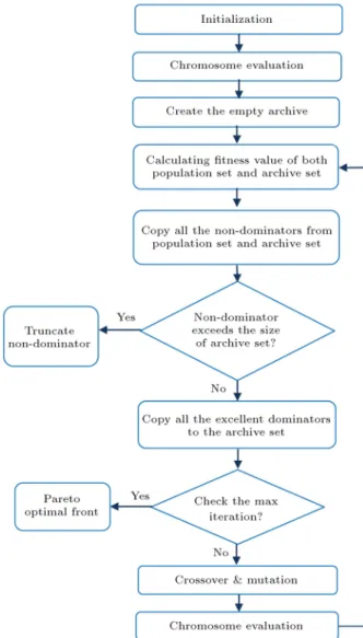
The owchart of this algorithm is presented in Figure 6. 4.2. Non-dominated Sorting Genetic

Algorithm (NSGA-II)

Deb et al. [43] were the rst to introduce NSGA-II. This algorithm is one of the most ecient multi-objective evolutionary algorithms to obtain Pareto optimal fronts for any number of objectives with any number of constrains. Due to its popularity and since NSGA-II is also a population-based algorithm, it is utilized in this research to validate the results obtained by SPEA-II.

Population ranking in NSGA-II is made according to two concepts: Fast Non-Dominated Sorting (FNDS) based on the domination concept and Crowding Dis-tance (CD) as a measure of solution density for solu-tions in the same fronts. Between two solusolu-tions that exist in a front, the one with the higher crowding distance is preferable [44]. In general, to determine whether a solution is dominated or not, all solutions are compared with each other to sort the population of size N, where the one that is not dominated by the other (front) is selected. The solutions in this set are the rst non-dominated bond. To determine the solutions in other bonds, the solutions of the rst bond are temporarily ignored and the process is repeated. This process is continued until the whole solutions stand in non-dominated bonds. To estimate solution density around a special solution, average distance of this solution from both adjoining solutions, called crowding distance, is computed. In order to compute

Figure 6. Flowchart of SPEA-II.

the crowding distance of a special solution in a bond, the largest rectangle in which the special solution lies within and the two adjoining solutions located in its two sides are considered. The summation of the length and the width of the rectangle are then the crowding distances of the special solution [43].

In order to compute crowding distances, the population is rst arranged in an ascending order according to their objective function values. Then, the crowding distances of the solutions in the rst and end of each bond (solutions with maximum and minimum objective function values) become innite. In this algorithm, n[j]distance represents mth objective

function value for ith member in set n. A solution with minimum crowding distance expresses a higher density around the solution. So, in the next step, it is desirable to select solutions that are in a region with lower density or, in other words, with a higher crowding distance. By this method, a greater variety of solution distributions become available [43]. The transmutation mechanism of NSGA-II is shown in Figure 7.

Figure 7. The transmutation process of NSGA-II [43].

In Figure 7, the parent population includes the primal population in each iteration. The ospring population is then generated by the crossover and mu-tation operations and the two population are merged to create a larger population. Next, FNDS is performed and the merged solutions are sorted in multiple fronts. After ranking the population in separate fronts using FNDS, the whole population in front1 and front2 are transferred to the next iteration. Moreover, a part of front3 with higher crowding distance is also transferred to the next iteration, and this trend continues until the optimal front is found. The owchart of this algorithm is presented in Figure 8.

Figure 8. Flowchart of NSGA-II.

4.3. Solution encoding

The initial population in both algorithms is rst gener-ated randomly. Then, a number of parents are selected based on the binary tournament selection method. Finally, the crossover and mutation operators act on the selected parents as follows.

ˆ Crossover operator: The uniform crossover oper-ator used in [19] is employed in this paper. In this operator, a binary random number is generated for each gene in the parent's chromosome. If this num-ber is one, then the values of the parent genes are exchanged with each other. Otherwise, if it is zero, then the replacement is not performed. Figure 9 demonstrates this operation in both algorithms. ˆ Mutation operator: In the mutation operation of

this research, a random number is rst generated for each gene of a parent. If this number is less than the mutation rate (mutation rate in this paper is 0.1), then the gene is mutated randomly [19]. The mutation operation of both algorithms is illustrated in Figure 10.

5. Numerical examples

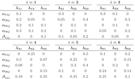
Some randomly generated numerical examples are solved in this section to not only validate the results obtained using SPEA-II, but also to evaluate the performances of the two algorithms. Consider a system consisting of six subsystems. The interconnection costs, the three failure rates of the components, the four dierent versions of technical activities, and one organi-zational activity are shown in Table 3. Besides, Table 4 contains the eects of technical and organizational activities on each subsystem and its components. All of the numbers listed in Tables 3 and 4 are generated randomly using uniform distributions.

In order to compare the results obtained using the two algorithms, 20 test problems are used for the presented system at time t = 100. These problems are generated based on the upper and lower bounds of component costs in [32] using a uniform distribution, i.e., Uniform (12; 22). The component costs are shown in Table 5. Moreover, the minimum acceptable value of ki in each subsystem is k = [2 1 3 1 5 3] that is

obtained based on a uniform distribution. 5.1. Performance measures

The measures used for evaluating the performance of the two multi-objective evolutionary algorithms are: 1. Diversity: This metric evaluates the extension of

the Pareto front [38];

2. Spacing: This metric measures the standard devia-tion of the distances among soludevia-tions of the Pareto front [45];

Figure 9. Crossover operation of the two algorithms.

Figure 10. Mutation operation of the both algorithms. Table 3. Input parameters of the problem.

I

Interconnection costs

Variable cost of technical and organizational activities

Constant cost of technical and organizational activities

The three failure rates of components i Ckh1i Ckh2i Ckh3i Ckh4i Ck1i Cko1i Cko2i Cko3i Cko4i i1 i2 i3

1 0.1 5 3 4 2 11 2 2 1 1 0.008 0.004 0.006

2 0.2 4 5 6 3 12 1 1 2 2 0.006 0.003 0.005

3 0.1 2 1 1 3 15 2 2 3 1 0.009 0.0045 0.0055

4 0.15 5 5 3 2 19 2 2 3 3 0.009 0.005 0.007

5 0.25 2 2 3 3 20 4 4 3 5 0.005 0.002 0.004

6 0.1 6 1 3 3 25 2 2 1 3 0.007 0.002 0.004

Table 4. Eects of technical and organizational activities on subsystems and their components.

i = 1 i = 2 i = 3

11 12 13 21 22 23 31 32 33

1ij 0.1 0 0 0.3 0 0 0.3 0.1 0

2ij 0.2 0.05 0 0.05 0 0.4 0 0 0.3

3ij 0.2 0.1 0.1 0 0.1 0 0 0.1 0

4ij 0.3 0.1 0.2 0 0.1 0 0.05 0 0.2

_1ij 0 0 0.1 0.1 0.05 0.2 0 0.05 0

i = 4 i = 5 i = 6

41 42 43 51 52 53 61 62 63

1ij 0 0.25 0 0 0 0.5 0.1 0 0.2

2ij 0.5 0 0.07 0 0.25 0 0 0 0.15

3ij 0.08 0 0 0 0.3 0.4 0 0.2 0

4ij 0 0 0.15 0.1 0 0 0.24 0 0.14

Table 5. The components cost in each test problem.

I Test problem

1 2 3 4 5 6 7 8 9 10 11 12 13 14 15 16 17 18 19 20

1 18 12 21 18 14 19 15 18 15 14 17 18 19 19 17 19 16 21 22 21

2 20 17 14 13 19 21 16 21 13 20 22 19 21 22 22 21 13 13 13 13

3 22 22 13 19 22 17 13 19 18 16 19 21 17 20 13 13 12 17 14 13

4 15 13 14 22 17 19 12 22 19 14 21 13 14 12 13 13 22 18 14 18

5 13 15 12 13 16 22 12 13 21 14 18 17 12 12 18 18 20 14 12 19

6 12 20 18 16 18 20 15 14 18 14 20 19 18 15 19 19 15 12 18 18

Table 6. Performance measures to compare the two multi-objective optimization algorithms.

Metric Formula Description

Diversity [38] D =

s

m

P

j=1

max

i f

j

i min_i fij

2

Evaluates the spread of the curve (m is the number of objectives and fij is the ith

value of the jth objective)

Spacing [45]

S = s

1=(n 1)Pn

i=1 di

d2 di= min

k3n\k6=i m

P

j=1jf i j fjkj

d =Pn

i=1di=n

Evaluates uniformity of the distribution of solutions within a front (n denotes the size of the Pareto front) Number of non-dominated

solutions in nal Pareto (NOS) |

It measures the number of Pareto solutions

Mean Ideal Distance (MID) [46] MID = 1=NOSNOSP

i=1ci

Evaluates the closeness of solutions of a Pareto front with an ideal point (ci represents

the distance of each member of population from the best possible value)

Time | Computational time in second

number of the Pareto solutions in Pareto optimal front;

4. Mean Ideal Distance (MID): This measure evalu-ates the closeness of solutions of a Pareto front with an ideal point [46];

5. Time: This metric measures the CPU time of running the algorithms to obtain near-optimum solutions.

Table 6 summarizes these measures. Interested readers are referred to the references shown in the rst column of this table for more details.

5.2. Results

Both algorithms are coded in MATLAB Version 7.10.0.499, R2010a. The codes are executed on a

Pentium 4 computer with a 3GB RAM and 2 cores 2.40 GHZ CPU under Windows 7 operating system, where the mission time is set 100 hours. The results obtained by employing the two algorithms on the 20 test problems along with the averages of the metrics are shown in Table 7.

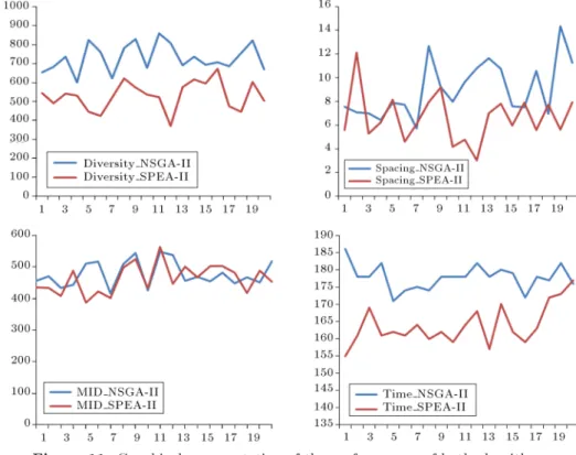
The results in Table 7 show that both algorithms have similar performances in terms of the NOS metric. However, while, based on the diversity metric, NSGA-II is the better algorithm, SPEA-NSGA-II shows better performances in terms of Spacing, MID, and Time metrics. These conclusions can be clearly seen in Figure 11. Moreover, Pareto solutions to four test-problem numbers 5, 10, 15, and 20 are shown in Figure 12, and the actual values of the objective functions for test problem #15 are presented in Table 8.

Table 7. The results obtained using the two algorithms based on the presented performance measures.

Test SPEA-II NSGA-II

Diversity" Spacing# NOS" MID# Time# Diversity" Spacing# NOS" MID# Time#

1 544.079 5.5728 50 434.859 155 653.422 7.5473 50 455.883 186

2 489.888 12.1197 50 432.942 161 683.514 7.0605 50 470.362 178

3 542.341 5.2803 50 408.385 169 735.975 7.0095 50 433.842 178

4 530.456 6.2072 50 487.664 161 599.794 6.4419 50 443.115 182

5 444.783 8.1653 50 387.801 162 823.840 7.8969 50 510.776 171

6 423.207 4.6155 50 422.551 161 760.160 7.7314 50 517.547 174

7 519.982 6.0948 50 401.988 164 621.419 5.7031 50 415.329 175

8 620.128 7.9404 50 496.963 160 780.629 12.6776 50 509.381 174

9 573.460 9.1757 50 524.917 162 829.809 9.2023 50 543.750 178

10 535.364 4.1593 50 432.531 159 678.245 7.9885 50 425.451 178

11 523.560 4.7657 50 563.705 164 859.267 9.6233 50 546.679 178

12 369.637 3.0433 50 446.802 168 807.757 10.7860 50 538.489 182

13 575.589 6.9892 50 500.620 157 691.043 11.6351 50 456.771 178

14 615.517 7.8024 50 466.830 170 734.899 10.7558 50 468.867 180

15 594.585 5.9494 50 501.839 162 694.547 7.5843 50 454.786 179

16 672.134 7.8882 50 503.074 159 705.465 7.5145 50 481.353 172

17 473.927 5.5913 50 481.354 163 685.569 10.5791 50 448.156 178

18 444.634 7.7175 50 418.204 172 754.681 6.9333 50 466.690 177

19 602.204 5.6084 50 487.498 173 820.475 14.3270 50 450.937 182

20 505.053 7.9379 50 452.204 177 670.149 11.2653 50 518.158 176

Average 530 6.631 50 462.6 163.95 729.5 9.013 50 477.82 177.8

#: Implies a negative metric (in this type of metric a lower value is desired); ": Implies a positive metric (in this type of metric a higher value is desired).

Figure 12. Examples of non-dominated solutions. Table 8. Pareto solutions to the test problem 15.

Solution NSGA-II SPEA-II Solution NSGA-II SPEA-II

Reliability Cost Reliability Cost Reliability Cost Reliability Cost

1 0 146.215 0.9457 739.728 26 0.1790 275.713 0.1123 264.125

2 0 146.215 0.9455 727.728 27 0.6861 428.348 0.5505 391.964

3 0.9582 824.46 0.9268 640.126 28 0.9432 715.46 0.7222 443.227

4 0.8056 499.227 0.9347 643.728 29 0.2760 305.998 0.3037 310.537

5 0.8865 552.96 0.9363 651.728 30 0.2072 286.207 0.0385 222.738

6 0.3353 314.614 0.9378 668.728 31 0.0430 207.894 0.6741 414.678

7 0.1277 252.307 0.9228 593.633 32 0.9244 648.46 0.6780 425.835

8 0.9516 789.46 0.9245 622.633 33 0.9399 681.46 0.7057 435.678

9 0.5581 374.183 0.0150 204.365 34 0.2986 310.756 0.7423 462.932

10 0.5014 355.026 0.4365 351.138 35 0.3924 335.884 0.2400 301.395

11 0.8308 533.129 0.9206 581.633 36 0.9434 734.46 0.1633 277.125

12 0.7057 445.504 0.9143 580.633 37 0.0715 251.036 0.8601 517.419

13 0.7396 455.053 0.0156 210.365 38 0.9088 600.46 0.9020 558.887

14 0.9059 577.46 0.4160 342.808 39 0.2424 296.478 0.6375 411.723

15 0.0194 186.766 0.3257 319.537 40 0.5974 388.032 0.7776 471.557

16 0.3923 324.884 0.0761 235.854 41 0.7673 466.227 0.1908 280.395

17 0.9474 759.46 0.5063 365.138 42 0.9384 666.46 0.8498 505.714

18 0.7753 474.227 0.0785 237.854 43 0.6731 412.428 0.8681 530.419

19 0.6412 398.174 0.0812 240.854 44 0.0660 249.036 0.8742 531.887

20 0.1527 267.571 0.0394 226.738 45 0.9213 625.46 0.8277 497.419

21 0.4404 339.026 0.3711 336.756 46 0.5974 388.032 0.7983 489.165

22 0.5346 362.183 0.0918 241.854 47 0.0211 193.766 0.8853 546.056

23 0.8354 542.96 0.1040 262.854 48 0.6480 412.174 0.8171 496.419

24 0.4682 341.884 0.5570 399.183 49 0.2351 289.842 0.8963 546.887

25 0.0565 222.023 0.5433 374.183 50 0.9144 617.46 0.8141 492.557

In order to compare the performances of the two solution algorithms statistically, four tests of hypoth-esis on the means of four performance measures are performed based on paired t-tests at = 0:05. A typical hypothesis in these tests is:

(

H0: NSGA-II = SPEA-II

Ha : NSGA-II6= SPEA-II

To this aim, the performance measures obtained using both algorithms (shown in Table 7) are normalized by

Table 9. Paired T -test on the mean diversity.

N Mean StDev SE Mean

NSGA-II 20 0.5797 0.0454 0.010

SPEA-II 20 0.47965 0.00983 0.010

Dierence = (NSGA-II) (SPEA-II)

H0 is rejected

Estimate for dierence: 0.1594 95% CI for dierence: (0.1303, 0.1884) T -test of dierence = 0 (vs not =): T -value = 11.11, P -value = 0.000 Df = 38

Table 10. Paired T -test on the mean spacing.

N Mean StDev SE Mean

NSGA-II 20 0.5766 0.0967 0.022

SPEA-II 20 0.4234 0.0967 0.022

Dierence = (NSGA-II) (SPEA-II)

H0 is rejected

Estimate for dierence: 0.1531 95% CI for dierence: (0.0913, 0.2150) T -test of dierence = 0 (vs not =): T -value = 5.01, P -value = 0.000 Df = 38

Table 11. Paired T -test on the mean MID.

N Mean StDev SE Mean

NSGA-II 20 0.5084 0.0266 0.060

SPEA-II 20 0.4916 0.0266 0.060

Dierence = (NSGA-II) (SPEA-II)

H0 is rejected

Estimate for dierence: 0.01671

95% CI for dierence: (-0.00034, 0.03377) T -test of dierence = 0 (vs not =): T -value = 1.98, P -value = 0.055 Df = 38

Table 12. Paired T -test on the mean CPU time.

N Mean StDev SE Mean

NSGA-II 20 0.52035 0.00983 0.0022

SPEA-II 20 0.47965 0.00983 0.0022

Dierence = (NSGA-II) - (SPEA-II)

H0 is rejected

Estimate for dierence: 0.04070

95% CI for dierence: (0.03441, 0.04700) T -Test of dierence = 0 (vs not =): T -value = 13.09, P -value = 0.000 Df = 38

dividing them by their totals in order to eliminate the eect of the size of the test problem solved.

The results, shown in Tables 9-12, indicate sig-nicant dierences between the means of diversity, spacing, and CPU time (the P -values of these tests are

less than the signicant level 0.05). However, there is no dierence between the two means of MID obtained. The interval-plots of all metrics shown in Figure 13 show that the above conclusion is better. In other words, NSGA-II works better in terms of diversity,

Figure 13. Interval plots of the means of the metrics.

while SPEA-II is the better algorithm in terms of the spacing and CPU time metrics.

6. Conclusion and future studies

One of the useful methods to increase system reliability is RAP. In modeling this type of problem, it is more realistic to optimize more than one objective simul-taneously. This paper aimed to solve a bi-objective optimization problem of a tri-state system consisting of several k-out-of-n subsystems connected in series. The components in each subsystem were assumed to have only three levels of performances degrading from fully working to failed states that would aect the system reliability over time. The system reliability could be improved by either adding redundant components or performing technical and organizational activities to change the transition rates of the components. The bi-objective optimization model that considered maximiz-ing system reliability and minimizmaximiz-ing total cost as two conicting objectives was developed. The two multi-objective algorithms, i.e. the Strength Pareto Evolu-tionary Algorithm (SPEA-II) and the Non-dominated Sorting Genetic Algorithm (NSGA-II), were used to solve the resulting optimization problem. The compar-ison study of the two algorithms in terms of ve multi-objective performance measures obtained using 20 test problems showed better performances of SPEA-II in most of the measures.

For future research studies in this area, we recom-mend the followings:

ˆ Considering repairable components;

ˆ Considering multiple types of components for sub-systems;

ˆ Considering failure rates of component as time-dependent;

ˆ Considering failure rates of components as random or fuzzy variables;

ˆ Extending the model by adding other constraints or other objective functions;

ˆ Using other meta-heuristic algorithms such as multi-objective simulated annealing, multi-objective biogeography-based optimization, and similar ones. Acknowledgement

The authors are grateful to the anonymous reviewers for their invaluable comments. Taking care of the com-ments improved the presentation signicantly. This research was nancially supported by Iranian National Science Foundation under grant number 92020691, for which the authors are thankful.

References

1. Fye, D.E., Hines, W.W. and Lee, N.K. \System reliability allocation and a computational algorithm", IEEE Transactions on Reliability, 17, pp. 64-69 (1968).

2. Nakagawa, Y. and Miyazaki, S. \Surrogate constraints algorithm for reliability optimization problems with two constraints", IEEE Transactions on Reliability, 30, pp. 175-180 (1981).

3. Buln, R.L. and Liu, C.Y. \Optimal allocation of re-dundant components for large systems", IEEE Trans-actions on Reliability, 34, pp. 241-247 (1985). 4. Misra, K.B. and Sharma, U. \Reliability optimization

of a system by zero-one programming", Microelectron-ics and Reliability, 31, pp. 323-335 (1991).

5. Bai, D.S., Yun, W.Y. and Chung, S.W. \Redundancy optimization of k-out-of-n systems with common-cause failures", IEEE Transactions on Reliability, 40, pp. 56-59 (1991).

6. Pham, H. \Optimal design of k-out-of-n redundant systems", Microelectronics and Reliability, 32, pp. 119-126 (1992).

7. She, J. and Pecht, M.G. \Reliability of a k-out-of-n warm-standby system", IEEE Transactions on Reliability, 41, pp. 72-75 (1992).

8. Pham, H. and Malon, D.M. \Optimal design of systems with competing failure modes", IEEE Transactions on Reliability, 43, pp. 251-254 (1994).

9. Coit, D.W. and Smith, A.E. \Optimization approaches to the redundancy allocation to the redundancy alloca-tion problem for series-parallel systems", Proceedings of the Fourth Industrial Engineering Research Confer-ence, Nashville TN, pp. 342-349 (1995).

10. Coit, D.W. and Smith, A.E. \Reliability optimization of series-parallel systems using a genetic algorithm", IEEE Transaction on Reliability, 45, pp. 254-260 (1996a).

11. Coit, D.W. and Liu, J. \System reliability optimization with k-out-of-n subsystems", International Journal of Reliability, Quality & Safety Engineering, 35, pp. 535-544 (2000).

12. Coit, D.W. \Maximization of system reliability with a choice of redundancy strategies", IEEE Transaction on Reliability, 35, pp. 535-544 (2003).

13. Tian, Z., Levitin, G. and Zuo, M. \A joint reliability-redundancy optimization approach for multi-state se-ries parallel systems", Reliability Engineering and Sys-tem Safety, 94, pp. 1568-1576 (2009).

14. Chern, M.S. \On the computational complexity of reliability redundancy allocation in a series system", Operation Research Letters, 11, pp. 309-315 (1992). 15. Ida, K., Gen, M. and Yokota, T. \System

reliabil-ity optimization with several failure modes by ge-netic algorithm", Proceeding of the 16th International Conference on Computers and Industrial Engineering, Ashikaga, Japan (1994).

16. Yokota, T., Gen, M. and Ida, K. \System reliability of optimization problems with several failure modes by genetic algorithm", Japanese Journal of Fuzzy Theory and Systems, 7, pp. 117-135 (1995).

17. Coit, D.W. and Smith, A.E. \Penalty guided genetic search for reliability design optimization", Computers and Industrial Engineering, 30, pp. 895-904 (1996b). 18. Coit, D.W. \Cold standby redundancy optimization

for non repairable systems", IEEE Transaction on Reliability, 33, pp. 471-478 (2001).

19. Tavakkoli-Moghaddam, R., Safari, J. and Sassani, F. \Reliability optimization of series-parallel systems with a choice of redundancy strategies using a genetic algorithm", Reliability Engineering and System Safety, 93, pp. 550-556 (2008).

20. Safaei, N., Tavakkoli-Moghaddam, R. and Kiassat, C. \Annealing-based particle swarm optimization to solve the redundant reliability problem with multiple component choices", Applied Soft Computing, 12, pp. 3462-3471 (2012).

21. Chambari, A., Naja, A.A., Rahmati, S.H.A. and Karimi, A. \An ecient simulated annealing algorithm for the redundancy allocation problem with a choice of redundancy strategies", Reliability Engineering and System Safety, 119, pp. 158-164 (2013).

22. Teimouri, M., Zaretalab, A., Niaki, S.T.A. and Shari, M. \An ecient memory-based electromagnetism-like mechanism for the redundancy allocation problem", Applied Soft Computing, 38, pp. 423-436 (2016). 23. Pourkarim Guilani, P., Azimi, P., Niaki, S.T.A. and

Niaki, S.A.A. \Redundancy allocation problem of a system with increasing failure rates of components based on Weibull distribution: A simulation-based optimization approach", Reliability Engineering and System Safety, 152, pp. 187-196 (2016).

24. Levitin, G., Lisnianski, A., Ben Haim, H. and Elmakis, D. \Redundancy optimization for series-parallel multi-state systems", IEEE Transactions on Reliability, 47, pp. 165-72 (1998).

25. Ramirez-Marquez, J.E. and Coit, D.W. \A heuristic for solving the redundancy allocation problem for multi-state series-parallel systems", Reliability Engi-neering and System Safety, 83, pp. 341-349 (2004). 26. Tian, Z. and Zuo, M. \Redundancy allocation for

multi-state systems using physical programming and genetic algorithms", Reliability Engineering and Sys-tem Safety, 91, pp. 1049-56 (2006).

27. Ushakov, I. \Universal generating function", Soviet J. Comput. Systems Sci., 24, pp. 118-129 (1986). 28. Levitin, G. and Lisnianski, A. \A new approach

to solving problems of multi-state system reliability optimization", Quality and Reliability Engineering In-ternational, 17, pp. 93-104 (2001).

29. Lisnianski, A. and Levitin, G. \Multi-state system re-liability: Assessment, optimization and applications", Singapore: World Scientic (2003).

30. Li, W. and Zuo, M. \Reliability evaluation of multi-state weighted k-out-of-n systems", Reliability Engi-neering and System Safety, 93, pp. 160-167 (2008). 31. Pourkarim Guilani, P., Shari, M., Niaki, S.T.A. and

Zaretalab, A. \Reliability evaluation of non-reparable three-state systems using Markov model and its com-parison with the UGF and the recursive methods", Reliability Engineering and System Safety, 129, pp. 29-35 (2014a).

32. Pourkarim Guilani, P., Shari, M., Niaki, S.T.A. and Zaretalab, A. \Solving the redundancy allocation problem for a system with three states components using genetic algorithm", International Journal of Engineering, 27, pp. 1663-1672 (2014b).

33. Chambari, A., Rahmati, S.H.A., Naja, A.A. and Karimi, A. \A bi-objective model to optimize relia-bility and cost of system with a choice of redundancy strategies", Computers and Industrial Engineering, 63, pp. 109-119 (2012).

34. Khalili-Damghani, K. and Amiri, M. \Solving binary-state multi-objective reliability redundancy alloca-tion series-parallel problem using ecient epsilon-constraint, multi-start partial bound enumeration al-gorithm, and DEA", Reliability Engineering and Sys-tem Safety, 103, pp. 35-44 (2012).

35. Safari, J. \Multi-objective reliability optimization of series-parallel systems with a choice of redundancy strategies", Reliability Engineering and System Safety, 108, pp. 10-20 (2012).

36. Khalili-Damghani, K., Abtahi, A.R. and Tavana, M. \A decision support system for solving multi-objective redundancy allocation problems", Quality and Relia-bility Engineering International, 30(8), pp. 1249-1262 (2014).

37. Wang, Z., Chen, T., Tang, K. and Yao, X. \A multi-objective approach to redundancy allocation problem in parallel-series systems", Proceedings of the 10th IEEE Congress on Evolutionary Computation (CEC '09), Trondheim, Norway (2009).

38. Zitzler, E. \Evolutionary algorithms for multi-objective optimization: method and applications", Ph.D. Thesis, dissertation ETH NO. 13398, Swaziland Federal Institute of Technology Zorikh, Switzerland, (1999).

39. Zitzler, E., Laumanns, M. and Thiele, L. \SPEA-II: Improving the strength Pareto evolutionary algo-rithm", In Computer Engineering and Networks Lab-oratory, Swiss Federal Institute of Technology (ETH), Zurich, Switzerland, TIK Report 103 (2001).

40. Wei, Z., Feng, Y. and Tan, J. \Research on quality performance conceptual design based on SPEA-II+", Computers and Mathematics with Applications, 57, pp. 1943-1948, (2009).

41. Sheng, W., Liu, Y., Meng, X. and Zhang, T. \An improved strength Pareto evolutionary algorithm 2 with application to the optimization of distributed generations", Computers and Mathematics with Appli-cations, 64, pp. 944-955 (2012).

42. Silverman, B.W., Density Estimation for Statistics and Data Analysis, London, Chapman and Hall (1986). 43. Deb, K., Agrawal, S., Pratap, A. and Meyarivan, T. \A

fast elitist non-dominated sorting genetic algorithm for multi-objective optimization: NSGA-II", In Proceed-ings of the Parallel Problem Solving from Nature VI (PPSN-VI) Conference, pp. 849-858 (2000).

44. Deb, K., Agrawal, S., Pratap, A. and Meyarivan, T. \A fast and elitist multiobjective genetic algorithm: NSGA-II", IEEE Transactions on Evolutionary Com-putation, 6, pp. 182-197 (2002).

45. Schott, J.R. \Fault tolerant design using single and multicriteria genetic algorithms optimization", Mas-ter's Thesis, Department of Aeronautics and Astro-nautics, Massachusetts Institute of Technology, Cam-bridge, MA (1995).

46. Zitzler, E. and Thiele, L. \Multiobjective optimization using evolutionary algorithms: a comparative case study", In Fifth International Conference on Parallel Problem Solving from Nature (PPSN-V), A.E. Eiben, T. Back, M. Schoenauer and H.P. Schwefel, Eds., Berlin, Germany, pp. 292-301 (1998).

Biographies

Pedram Pourkarim Guilani is a PhD candidate at the Faculty of Industrial and Mechanical Engineering in Qazvin Islamic Azad University, Qazvin, Iran. He holds BSc and MSc degrees, both in Industrial Engi-neering, from Qazvin Islamic Azad University. His ar-eas of interests include reliability theory, optimization via simulation, meta-heuristic algorithms, and Markov theory.

Arash Zaretalab is a PhD candidate at the Depart-ment of Industrial Engineering, Amirkabir University of Technology, Tehran, Iran. He received his BSc and MSc degrees, both in Industrial Engineering, from Qazvin Islamic Azad University. His areas of interests include reliability theory, meta-heuristic algorithms, supply chain management, and queuing theory. Seyed Taghi Akhavan Niaki received his BS degree in Industrial Engineering from Sharif University of Technology, Tehran, Iran, in 1979, and his MS and PhD degrees, both in Industrial Engineering, from West Virginia University, USA, in 1989 and 1992, respectively. He is, currently, Distinguished Professor of Industrial Engineering at Sharif University of Tech-nology, Tehran, Iran. His research interests include: simulation modeling and analysis, applied statistics, multivariate quality control, and operations research. Before joining Sharif University of Technology, he worked as a Systems Engineer and Quality Control Manager for the Iranian Electric Meters Company. He is also a member of .

Pardis Pourkarim Guilani holds BSc and MSc degrees, both in Industrial Engineering, from Faculty of Engineering, Kharazmi University, Tehran, Iran. Her areas of interests include reliability theory and meta-heuristic algorithms.