ISSN: 2252-8938, DOI: 10.11591/ijai.v8.i2.pp144-155 144
Hybrid imperialistic competitive algorithm incorporated with
hopfield neural network for robust 3 satisfiability logic
programming
Vigneshwer Kathirvel1, Mohd. Asyraf Mansor2, Mohd Shareduwan Mohd Kasihmuddin3,
Saratha Sathasivam4
1,3,4Schoolof Mathematical Sciences, Universiti Sains Malaysia, 11800 USM, Pulau Pinang, Malaysia 2School of Distance Education, Universiti Sains Malaysia, 11800 USM, Pulau Pinang, Malaysia
Article Info ABSTRACT
Article history: Received Jan 30, 2019 Revised Apr 28, 2019 Accepted May 17, 2019
Imperialist Competitive algorithm (ICA) is a robust training algorithm inspired by the socio-politically motivated strategy. This paper focuses on utilizing a hybridized ICA with Hopfield Neural Network on a 3-Satisfiability (3-SAT) logic programming. Eventually the performance of the proposed algorithm will be compared to other 2 algorithms, which are HNN-3SATES (ES) and HNN-3SATGA (GA). The performance shall be evaluated with the Root Mean Square Error (RMSE), Mean Absolute Error (MAE), Sum of Squares Error (SSE), Schwarz Bayesian Criterion (SBC), Global Minima Ratio and Computation Time (CPU time). The expected outcome will portray that the IC algorithm will outperform the other two algorithms in doing 3-SAT logic programming.
Keywords: 3 Satisfiability Exhaustive search Hopfield neural network Imperialistic competitive algorithm
Logic programming
Copyright © 2019 Institute of Advanced Engineering and Science. All rights reserved.
Corresponding Author: Vigneshwer Kathirvel,
School of Mathematical Sciences, Universiti Sains Malaysia, 11800 USM, Penang, Malaysia. Email: [email protected]
1. INTRODUCTION
Our biological neural network’s structure have inspired new models of computing to perform pattern recognition tasks. However, the operations of the biological neuron and the neural interconnections are not fully understood till this very day [1]. It automatically adapts to a new environment without being reprogrammed, and it is able to deal with fuzzy, probabilistic, noisy and inconsistent information [2]. Artificial intelligence attracted a profuse number of research in combinatorial optimization problems [3]. Artificial intelligence became popular among researches due to its capability to solve computational, classification and pattern recognition problems using learning based algorithm. Its architecture consists of a two-dimensional connecter neural network in which linking the strengths between neurons are decided based on the constraints and solution basis of the optimization problem to be solved [4].
One of the most commemorated topics is the satisfiability problem (SAT). The SAT problem can be distinguished as the process of obtaining an ideal assignment using Boolean values to corroborate that the formula is satisfied [5]. In this paper, we shall stress on 3-Satisfiability, or commonly known as 3-SAT. 3-SAT can be defined as a formula in conjunctive normal form (CNF) whereby each of the number of neurons are limited to 3 literals or neurons. Exhaustive search, or commonly known as brute-force search, is a very conventional problem-solving method and algorithmic paradigm that is comprised of systematically identifying all possible candidates for the solution and to clarify whether or not the candidates satisfies
the problem statement respectively [6]. HNN-3SATES is a popular algorithm-design as it is widely applicable and given correct generation and checking.
In Riddle’s and Segal’s paper, they have applied inductive categorization methods in a set of data collection in a Boeing plant with the objective of unveiling the possible flaws or setback in a manufacturing process. Two experiments were carried out [7] which would test the predictions extracted from the assumptions that lexical access includes a search process are reported. It is also shown that when the target of the search is a non-existent entry, it involves an HNN-3SATES, although the test items are words. From the results of the experiment, it was deduced that the search model explains the procedure adequately, where the most known meaning of a homograph is accessed [8]. The Imperialist competitive algorithm (ICA) is inspired by the human socio-political evolution process. In Lucas’ and Nasiri’s paper, a novel optimization algorithm based on HNN-3SATICA algorithm is used for the design of a low speed single sided linear induction motor (LIM) [9]. Having high efficiency with high power factor is very vital in these applications. The results shows that ICA is more successful for the design of LIMs compared to genetic algorithm (GA) and conventional design [10]. This meta-heuristic solution approach is also used to optimize product mix-outsourcing for manufacturing enterprises. In Miller’s paper, they have combined two adaptive processes, the genetic search through the network architecture space, and backpropagation learning in individual networks. Cycles of learning in individuals are nested within cycles of evolution in populations, and each of the learning cycle presents an individual neural network, with the set of input-output pairs defining the task [11]. Lam’s paper on the other hand presents the tuning of the structure and parameters of a neural network using an improved GA. The structure and parameters of the neural network can be tuned using the improved GA [12]. In this paper, we will develop hybrid model of ICA with Hopfield in 3-SAT (HNN-3SATICA). The comparison will be between the hybrid exhaustive search (HNN-3SATES) and hybrid genetic algorithm(HNN-3SATGA).
2. RESEARCH METHODS
2.1. 3-Satisfiability
The 3-SAT paradigm allows binary values of each variable, which consist of either 1 or -1. The 3-SAT problem can be sealed as a non-deterministic problem [13]. The 3-SAT problem in the conjunctive normal form (CNF) comprises of four radical features:
1. The SAT formula has an array of n variables, z z1, ,....,2 zn inside of each number of neurons. In this case, we shall limit it to at most 3 (n3).
2. A set of m number of neurons in a Boolean formula, m F: c1 c2 .... cm.
3. We considered 3 literals in each number of neurons in 3-SAT. Each number of neurons, ckwill be combined by the logic operator OR.
4. The literals can be the variables or the negation of the variables itself. The 3-SAT formula can be illustrated as per the following:
P A B C D E F G H I (1)
The formula can generally be created in multiple combinations as the number of atoms may vary. Relatively, the probabilities of a number of neurons to be satisfied will be maximized by the greater number of literals per number of neurons [14].
2.2. Hopfield neural network
Recurrent neural networks are primarily dynamical systems that feedback signals to themselves. Popularized by John Hopfield, these models have a rich class of dynamics characterized by the existence of a few stable states, having their respective basin of attraction [15]. Show in Figure 1 Hopfield Neural Network. These interconnected units are also known as the bipolar threshold unit. Here, the binary values are considered to be 1 or -1 [16]. Hence, Ni will be the ith activation of a neuron, having the following threshold function:
1 ,
1 ,
ij j i i
if w S N Otherwise
(2)where wij is the connection strength from unit j to i. Sjrepresents the unit of j andi represents the threshold of unit i. There are no connections within the connection in the Hopfield net usually, hence wij 0. This shows that the connections are bidirectional or symmetric wijwji [17]. Neuron is in general bipolar,
{1, 1} i
S which fulfils the dynamics Sisgn( )hi , where the local field is represented by hi. The computational model will directly approximate to a higher order connection. Therefore, the local field modifies to the following:
(3) (2) (1)
i ijk j k ij j i
j j
h
w S S
w S w (3)The energy function by Pinkas (1991) for the discrete Hopfield Neural Network for 3-Satisfiability number of neurons can be written as follows:
(3) (2) (1)
1 1
3 ijk i j k 2 ij i j i j
i j k i j i
E
w S S S
w S S
w S (4)Hopfield’s energy function is particularly vital as it will determine the degree of convergence of the network[18]. The energy value attained from the equation will be checked and determined whether it is a global or a local minima.
Figure 1. Hopfield neural network [7]
2.3. Exhaustive search algorithm
The purpose for choosing this typical algorithm is to discover the effectiveness degree of HNN – 3SATES. Apart from that, there are theoretically satisfying assignments given for any 3-SAT problem [19]. The satisfied assignment for the ES algorithm is obtained after conducting a brutal “trial and error” procedure. The performance of ES has already been reconnoitred in the work of Nievergelt (2000). The objective function is demonstrated as the following:
max{fES} (5)
Herewith are the steps of implementing ES: Stage 1: Initialization
The candidate bit string is initiated and generated. Stage 2: Fitness Evaluation
The candidate bit string is tested and hence, the fitness will be computed by utilizing the following:
1( ) 2( ) 3( ) ... ( )
ES total NC
f c x c x c x c x (6)
Stage 3: Evaluation
As an outcome, return the assignment with the maximum fitness. Else otherwise, identify a new candidate bit string.
2.4. Imperialist competitive algorithm
HNN-3SATICA algorithm is a new meta-heuristic optimization developed based on a sociopolitically motivated strategy and contains two main steps [20]:
The movement of the colonies The imperialistic competition
It is a brand new evolutionary technique galvanized by the imperialistic competition among nations. The initial population of solution is represented as country.
Here are the 6 main stages of ICA: Stage 1: Initialization
The parameters are determined and the country’s population are initialized. For instance, Country = 100.
1 2 3
( , , ,.... )n
country x x x x (7)
Stage 2: Fitness of the Countries
The fitness of the countries are calculated.
1( ) 2( ) 3( ) ... ( )
country total NC
f c x c x c x c x (8)
Stage 3: Imperialist Selection
Generate the empire. The imperialist will be selected from the country with the highest fitness and the others remain as colonies.
Stage 4: Assimilation
Select N=5 from the most powerful countries to form empires. The remaining countries or colonies shall be designated to these empires respectively.
Stage 5: Revolution
This is where there will be an exchange in position between a colony and the Imperialist. A colony that possess a better position will have the likelihood to take charge of the empire by replacing the existing Imperialist.
Stage 6: Imperialistic Competition
This would be the crucial stage, whereby all imperialist will compete to take control of each other’s colonies. The total power of the empire will be computed as follows:
{ }
n imperialist coloniesof empire
power f mean f (9)
where fimperialist indicates the fitness of each imperialist, fcolonies of empire represents the fitness of the colonies of the empire and ε = 0.05 refers to a IC free parameter. Empires which are powerless will fall in the imperialistic competition and the imperialist with the highest power will be chosen as the surviving imperialist. Repeat step 5 if the highest power consists of fimperialist mean f{coloniesof empire} . The solution will be then stored in HNN.
2.5. Genetic algorithm
The HNN-3SATGA (GA) are algorithms for optimization and learning based entirely on a few biological evolution features [21]. This algorithm requires mainly 5 components:
A method of encoding solutions to the problem on chromosomes
An evaluation function that returns a rating for each chromosome given to it A way of developing the population of chromosomes
Operators that may be applied to parents when they reproduce to modify their genetic composition. Parameter settings for the algorithm, operators and others.
There are principally 5 stages in the process of GA: Stage 1: Initialization
100 populations of chromosomes randomized as the interpretations (bit strings). Hence, the probable interpretation of EHNN-3SAT will be depicted by the chromosomes.
Stage 2: Fitness Evaluation
The fitness of the chromosomes are computed based on the number of satisfied number of neurons in each of the exposition. The training process’ effectiveness will be determined by the maximum fitness.
Stage 3: Selection Stage
10 prospect chromosomes out of the 100 that are noted to have maximum fitness will advance to the following generation and stage of GA. Later on, these chosen chromosomes will carry out the crossover procedure to amplify the fitness and variability.
Stage 4: Crossover
The crossover operator includes the main transformation steps in the HNN-3SATGA. Information exchange will occur during this phase between two sub-structure of the chromosomes (bit strings). The crossover point chromosomes is defined mutably to sustain the chromosomes genetic diversity. Crossover normally increases the number of satisfied number of neurons of the new chromosome pairs. Stage 5: Mutation
The non-improving interpretations that still exists will be enhanced by mutation. The mutation in GA entails the flipping of the state of the bit string, either from 1 to -1 or vice versa. This will result in a better chromosome being generated after mutation. Since the mutation has occurred, the fitness value will have to be re-evaluated for the newly formed chromosomes. The stages shall repeat from stage 1 if the maximum fitness value is not attained.
3. PERFORMANCE EVALUATION MATRIX
In this paper, we shall utilize C++ to run the 3-SAT problem using the above mentioned algorithms. In order to verify which algorithm shall outperform the rest, a series of performance evaluation shall determine which would be the better algorithm to be used.
3.1. Root mean square error
Root Mean Square Error, or commonly known as RMSE, is widely used to measure the differences between predicted values of a model and the actual values. They suggested that RMSE is more suitable to represent model performance when the distribution of the error is anticipated to be Gaussian. RMSE is defined [22] as follows:
2 max 1 1 ( ) n i i
RMSE f f
n
(10)3.2. Mean absolute error
The measure of differences between two continuous variable is known as the Mean Absolute Error (MAE). Unlike RMSE, the calculation of MAE is relatively simple, whereby the magnitudes are summed (absolute values) of the errors to attain the cumulative error [23]. The MAE formula is described as the following: max 1 1 n i i
MAE f f
n
(11)Similarly, thefi represents the fitness value observed, whereas the fmax will be the maximum fitness.
3.3. Sum of squares error
This error is to measure how far the data are from the assumed values of the model. A sum of squares (SSE) minimum can frequently be searched very efficiently via application of a generalization of the least square method [24]. The generated the formula of SSE as below:
2 max 1 ( ) n i i
SSE f f
(12)The fi represents the fitness value observed, whereas the fmaxwill be the maximum fitness 3.4. Schwarx bayesian criterion
Schwarz Bayesian Criterion (SBC), or also called Bayesian Information Criterion (BIC), is a criterion for selecting models from a finite set of models [25]. When models are fitted, it is likely to increase
when the parameters are added. They have taken the model comparison approach to analysing statistically [26]. Assuming that the disturbances or model errors are independent and distributed equally in accordance to a normal distribution and that the condition of the boundary that the log’s derivative with respect to the true variance is zero, the formula generated will be:
.ln( ) .ln( )
SBCn MSE pa n (13)
The n represents the number of solutions, pa would be the number of parameters and MSE is the mean square error.
3.5. Computation time
Computation time or widely known as CPU time (also called running time) is the measure of time required to perform a computational process [27]. It is proportional to the number of rule applications and the computation time is measured using seconds. Computation time is defined by the following equation.
_ ( ) _ ( ) _ ( )
CPU Time s Training Time s Retrieval Time s (14)
3.6. Global minima ratio
The global minima ratio is defined by the ratio of the cumulative global minimum energy to the number of trials or number of neurons [28]. It will be feasible to indicate the simulation by checking the global minima ratio since the program is seeking for every neuron’s state global minimum energy in 3-SAT[29]. The equation of global minima ratio is given by the following.
min 1
1
( )( )
n
E i
Global Minima Ratio N
NTr COMBMAX
(15)NTr indicates the number of trials,NEminis the global minimum solutions and COMBMAX is the neuron’s maximum combination.
4. METHODOLOGY/IMPLEMENTATION
HNN – 3SATES, HNN – 3SATGA and HNN – 3SATICA will be proposed to evaluate the performance. The implementation of these models to the 3-SAT problem will be according to the flow chart:
5. RESULTS AND ANALYSIS
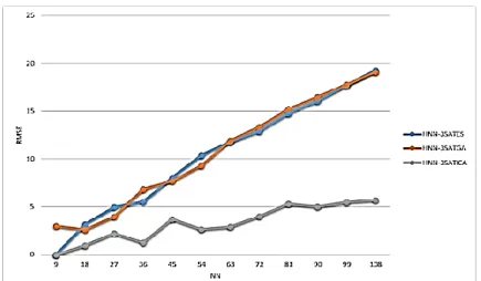
The simulations of the 3-SAT problem using various algorithms was conducted with an Intel® Core™ [email protected], 4.00GB RAM ASUS A556U Series, via DEV C++. From the training phase illustrated in Figure 2, observed that after 12 number of neurons, the HNN-3SATES algorithm produce the highest number of errors. It showed a close proportionate relationship between the number of number of neurons and errors obtained. This similar pattern was also portrayed at the testing phase for ES in Figure 3,
but there were some mild fluctuations in the error readings. HNN-3SATGA, on the other hand, showed a more consistent increase as the number of number of neurons got higher.
However, this pattern is not the same in the testing phase. As observed, there is quite a significant variation of the errors for the first 5 to 6 number of neurons, and eventually becomes consistent and closing to the performance of the ES algorithm. HNN-3SATICA algorithm seemed a little more compelling compared to the other 2 algorithms. In the training phase, it showed an absolute 0 error throughout the number of neurons, and a very minimal error trend on the testing phase in comparison with ES and GA. On the training phase, it is observed that HNN-3SATES algorithm had a huge value until the value of NN=108. The possibility of obtaining the correct interpretations will reduce drastically when there is an increase in the number of neurons. This is due to its nature that kicks off the “generate and test” and “trial and error” technique in order to attain the correct solutions in a specific search space.
Figure 2. RMSE evaluation of HNN-3SATES, HNN-3SATGA & HNN-3SATICA training phase
Figure 3. RMSE evaluation of HNN-3SATES, HNN-3SATGA & HNN-3SATICA-testing phase
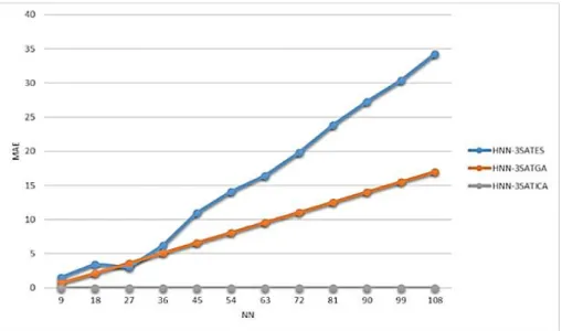
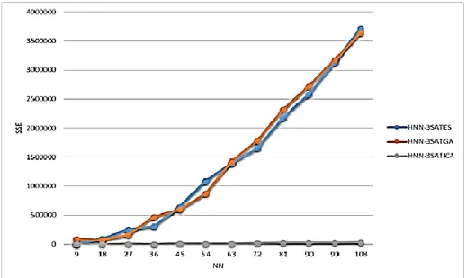
Shown in Figure 4, the ES algorithm again portrayed the highest number of errors, followed by the GA algorithm. The IC algorithm displayed absolutely no errors throughout the run. However, this is different in the testing phase as shown in Figure 5, whereby all 3 algorithms exhibit a very similar trend amongst each other. IC algorithm shows a drastic undulation on an increasing manner throughout the 12 number of neurons, but mostly having an error lower to that of GA and ES, where this 2 shows a more steady increase. As plotted, the ES again shows the highest number of errors produced, reaching slightly more than 1200 in the training phase and about 3600000 in the testing phase, as portrayed in Figure 6 and Figure 7. respectively. GA is significantly lower in the training phase, almost 3 times lower than ES, but shows a very homogenous
result to ES. IC, otherwise, proves to be a more stable run when it produces 0 errors again in the training phase, and almost 100 times lesser compared to ES and GA in the testing phase. From this, it can be deduced that the errors accumulated when the 3-SAT was trained and tested with GA and ES. This is different for IC where it was sustaining a very low value of errors. In other words, the compilation of errors was lesser with the increase of NN. Compared to ES and GA, the IC algorithm entailed lesser iterations to compute the desired solutions. ES in this case needed more iterations to attain a global solution, as the interpretation will disintegrate if it does not succeed to achieve the maximum fitness. This will then lead to the hunting of new interpretation with a new fitness value.
Figure 4. MAE evaluation of HNN-3SATES, HNN-3SATGA & HNN-3SATICA-training phase
Figure 6. SSE evaluation of HNN-3SATES, HNN-3SATGA & HNN-3SATICA - training phase
Figure 7. SSE evaluation of HNN-3SATES, HNN-3SATGA & HNN-3SATICA - testing phase
From Figure 8, when the number of neurons is 1, ES and IC were able to attain a global minima ratio of 1, except for GA. As the number of number of neurons increases till 12, it can be seen that the ratio gradually decreases for ES and GA. On the contrary, even with a reducing ratio, the IC algorithm tends to make an attempt to attain a ratio of 1, or at least close to it. This can be seen along the run that the readings are actually varying. At the 12th number of neurons, ES, GA and IC are approximately at the same value, but IC having a slightly higher ratio in comparison with the other 2 algorithms. In IC algorithm, it has a higher efficiency to neuro-searching method generated in comparison with ES and GA. The network became significantly became more complicated as the number of neurons increased, as the size of the restrictions became larger indefinitely. The system was also able to categorize feasible solutions constructively and adapt with more constraints. From the graph displayed in Figure 9, the ES algorithm shows the lowest SBC value at the 1st number of neuron, which is at the negative value, whereas IC is slightly below 0, while GA is already at 20000. The HNN-3SATICA is more effective in seeking for the correct interpretation without the use of more iterations. HNN-3SATES on the other hand penalized the SBC values due to the collection of MSE and retrieval phase. This explains the higher values of SBC in HNN-3SATES compared to the other two algorithms.
Figure 8. Global Minima Ratio of HNN-3SATES, HNN-3SATGA & HNN-3SATICA
Figure 9. SBC of HNN-3SATES, HNN-3SATGA & HNN-3SATICA
The speed of the ES and GA algorithm are notably similar in the 12 different number of neurons shown in Figure 10. It shows that when these algorithms are utilized for more number of neurons, the time taken will gradually increase as what is shown in the graph. The time taken for the IC algorithm is impressively low, even at the 12th number of neurons, marking at almost only 24 seconds. The power of the algorithm is basically demonstrated by the effectiveness of the computation process in whole. Therefore, particular accelerating system is required for the training process. The time of computation was higher for HNN-3SATICA due to the effectiveness of the imperialist to improve towards the preferred solutions. GA is comparatively similar, yet in real is still lower than ES, as the crossover and mutation processes have the ability to improve the interpretations. The ES brute force needed much more computation time as the “generate and test” system required more time to attain the correct interpretations.
Figure 10. Computation Time of HNN-3SATES, HNN-3SATGA & HNN-3SATICA
6. CONCLUSION
From the results obtained, it can be deduced that HNN-3SATICA algorithm has outperformed HNN-3SATES algorithm and HNN-3SATGA. This can be observed when the ICA has the least computation time, the lowest SBC value and most importantly, is able to generate a global minima ratio of 1. The errors are as well comparatively low, mainly on the testing phases as it was absolutely free from errors in the training phase. This also concludes that ICA is much more stable in terms of running a 3-SAT problem for a Hopfield Neural Network, and it is closest to achieving the global minima, regardless of the number of number of neurons generated. This work can be further explored by utilizing the other counterparts of 3-SAT, such as MAX-3-SAT, MIN-3-SAT and weighted 3-SAT. Additionally, other metaheuristic methods can be deployed in accelerating the computational process.
ACKNOWLEDGEMENTS
This research is supported by Universiti Sains Malaysia and Fundamental Research Grant Scheme (FRGS) (203/PMATHS/6711689) by Ministry of Higher Education Malaysia.
REFERENCES
[1] Sathasivam, S., 2010. Upgrading logic programming in Hopfield network. Sains Malaysiana, 39(1), 115-118.
[2] Sathasivam, S. and Abdullah, W.A.T.W., 2008. Logic learning in Hopfield networks. arXiv preprint arXiv:0804.4075.
[3] Mansor, M.A.B., Kasihmuddin, M.S.B.M. and Sathasivam, S., 2017. Robust Artificial Immune System in the Hopfield network for Maximum k-Satisfiability. IJIMAI, 4(4), 63-71.
[4] Liao, X. and Yu, J., 1998. Robust stability for interval Hopfield neural networks with time delay. IEEE Transactions on Neural Networks, 9(5), 1042-1045.
[5] Park, J.H., Kim, Y.S., Eom, I.K. and Lee, K.Y., 1993. Economic load dispatch for piecewise quadratic cost function using Hopfield neural network. IEEE transactions on power systems, 8(3), 1030-1038.
[6] Lee, K.Y., Sode-Yome, A. and Park, J.H., 1998. Adaptive Hopfield neural networks for economic load dispatch. IEEE transactions on power systems, 13(2), 519-526.
[7] Hopfield, J.J., 1982. Neural networks and physical systems with emergent collective computational abilities. Proceedings of the national academy of sciences, 79(8), 2554-2558.
[8] Kechriotis, G.I. and Manolakos, E.S., 1996. Hopfield neural network implementation of the optimal CDMA multiuser detector. IEEE Transactions on Neural Networks, 7(1), 131-141.
[9] Zhu, Y. and Yan, Z., 1997. Computerized tumor boundary detection using a Hopfield neural network. IEEE transactions on medical imaging, 16(1), 55-67.
[10]Luo, Z. and Liu, H., 2006, July. Cellular HNN-3SATGAs and local search for 3-SAT problem on graphic hardware. In Evolutionary Computation, 2006. CEC 2006. IEEE Congress on (2988-2992). IEEE.
[11]Hofmeister, T., Schöning, U., Schuler, R. and Watanabe, O., 2002, March. A Probabilistic 3—SAT Algorithm Further Improved. In Annual Symposium on Theoretical Aspects of Computer Science (192-202). Springer, Berlin, Heidelberg.
[12]Gu, J., Purdom, P.W., Franco, J. and Wah, B.W., 1999. Algorithms for the satisfiability (sat) problem. In Handbook of Combinatorial Optimization (379-572). Springer, Boston, MA.
[13]Friedgut, E. and Bourgain, J., 1999. Sharp thresholds of graph properties, and the 𝑘-sat problem. Journal of the American Mathematical Society, 12(4), 1017-1054.
[15]Anantharaman, T., Campbell, M.S. and Hsu, F.H., 1990. Singular extensions: Adding selectivity to brute-force searching. Artificial Intelligence, 43(1), 99-109.
[16]Morton, A.B. and Mareels, I.M., 2000. An efficient brute-force solution to the network reconfiguration problem. IEEE Transactions on Power Delivery, 15(3), 996-1000.
[17]Srinivasan, R. and Rao, K., 1985. Predictive coding based on efficient motion estimation. IEEE transactions on communications, 33(8), 888-896.
[18]Morris, G.M., Goodsell, D.S., Halliday, R.S., Huey, R., Hart, W.E., Belew, R.K. and Olson, A.J., 1998. Automated docking using a Lamarckian HNN-3SATGA and an empirical binding free energy function. Journal of computational chemistry, 19(14), 1639-1662.
[19]Deb, K., Agrawal, S., Pratap, A. and Meyarivan, T., 2000, September. A fast elitist non-dominated sorting HNN-3SATGA for multi-objective optimization: NSGA-II. In International Conference on Parallel Problem Solving From Nature (849-858). Springer, Berlin, Heidelberg.
[20]Jones, G., Willett, P., Glen, R.C., Leach, A.R. and Taylor, R., 1997. Development and validation of a HNN-3SATGA for flexible docking. Journal of molecular biology, 267(3), 727-748.s
[21]Xing, B. and Gao, W.J., 2014. Innovative computational intelligence: A rough guide to 134 clever algorithms, (203-209). Springer, Cham.
[22]Talatahari, S., Azar, B.F., Sheikholeslami, R. and Gandomi, A.H., 2012. Genetic algorithm combined with chaos for global optimization. Communications in Nonlinear Science and Numerical Simulation, 17(3), 1312-1319.
[23]Lucas, C., Nasiri-Gheidari, Z. and Tootoonchian, F., 2010. Application of an imperialist competitive algorithm to the design of a linear induction motor. Energy conversion and management, 51(7), 1407-1411.
[24]Ahmadi, M.A., Ebadi, M., Shokrollahi, A. and Majidi, S.M.J., 2013. Evolving artificial neural network and imperialist competitive algorithm for prediction oil flow rate of the reservoir. Applied Soft Computing, 13(2), 1085-1098.
[25]Willmott, C.J. and Matsuura, K., 2005. Advantages of the mean absolute error (MAE) over the root mean square error (RMSE) in assessing average model performance. Climate research, 30(1), 79-82.
[26]Chai, T. and Draxler, R.R., 2014. Root mean square error (RMSE) or mean absolute error (MAE)?. Geoscientific Model Development Discussions, 7, 1525-1534.
[27]Schwarz, G., 1978. Estimating the dimension of a model. The annals of statistics, 6(2), 461-464.
[28]Chen, J. and Chen, Z., 2008. Extended Bayesian information criteria for model selection with large model spaces. Biometrika, 95(3), 759-771.
BIOGRAPHIES OF AUTHORS
Vigneshwer Kathirvel was awarded a first class honors degree in Bachelors of Mechanical and Manufacturing Engineering (BSc) from Universiti Tun Hussein Onn Malaysia in the year 2014. He is currently pursuing his MSc in the School of Mathematics, Universiti Sains Malaysia in the field of Neural Network, Imperialist Competitive Algorithm, Artificial Intelligence and Logic.
Dr. Mohd. Asyraf Mansoris a lecturer in the School of Mathematical Sciences, Universiti Sains Malaysia. He received his Ph.D (2017), MSc (2014) and BSc(Ed) (2013) from Universiti Sains Malaysia. His current research interests include evolutionary algorithm, satisfiability problem, neural networks, logic programming and heuristic method.
Dr. Mohd Shareduwan Mohd Kasihmuddinis a lecturer in the School of Mathematical Sciences, Universiti Sains Malaysia. He received his Ph.D (2017), MSc (2014) and BSc(Ed) (2013) from Universiti Sains Malaysia. His current research interests include neuro-heuristic method, constrained optimization, neural network modelling algorithm and logic programming.
Assoc. Prof. Dr. Saratha Sathasivam is a lecturer in the School of Mathematical Sciences, Universiti Sains Malaysia. She received her MSc and BSc(Ed) from Universiti Sains Malaysia. She received her Ph.D at Universiti Malaya, Malaysia. Her current research interest are neural networks, agent based modeling and constrained optimization problem.
![Figure 1. Hopfield neural network [7]](https://thumb-us.123doks.com/thumbv2/123dok_us/8384728.2227776/3.893.275.644.533.714/figure-hopfield-neural-network.webp)