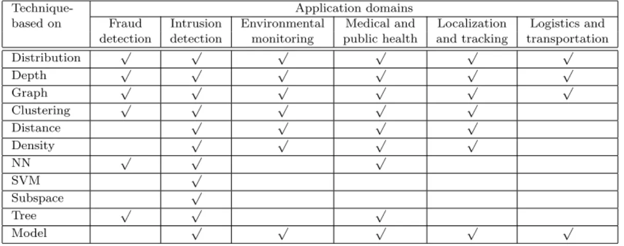
Detection Techniques for Multi-Type Data Sets
Yang Zhang, Nirvana Meratnia, Paul Havinga Department of Computer Science,
University of Twente, P.O.Box 217 7500AE, Enschede, The Netherlands
The term “outlier” can generally be defined as an observation that is significantly different from the other values in a data set. The outliers may be instances of error or indicate events. The task of outlier detection aims at identifying such outliers in order to improve the analysis of data and further discover interesting and useful knowledge about unusual events within numerous applications domains. In this paper, we report on contemporary unsupervised outlier detection techniques for multiple types of data sets and provide a comprehensive taxonomy framework and two decision trees to select the most suitable technique based on data set. Furthermore, we highlight the advantages, disadvantages and performance issues of each class of outlier detection techniques under this taxonomy framework.
Categories and Subject Descriptors: H.2.8 [Database Management]: Database Applications— data mining
General Terms: Algorithms, Performance
Additional Key Words and Phrases: Outlier, outlier detection, data mining
1. INTRODUCTION
Data mining, as a powerful knowledge discovery tool, aims at modelling relation-ships and discovering hidden patterns in large databases [1]. Among four typical
data mining tasks,outlier detection is the closest to the initial motivation behind
data mining than predictive modelling, cluster analysis and association analysis [2]. Outlier detection has been a widely researched problem in several knowledge
disci-plines, includingstatistics,data mining andmachine learning. It is also known as
anomaly detection, deviation detection, novelty detection and exception mining in some literature [3]. Being called differently, all these definitions aim at identifying instances of unusual behavior when compared to the majority of observations.
Coming across various definitions of an outlier, it seems that no universally ac-cepted definition exists. Two classical definitions of an outlier include Hawkins [4]
and Barnett and Lewis [5]. According to the former,“an outlier is an observation,
which deviates so much from other observations as to arouse suspicions that it was
generated by a different mechanism”, where as the latter defines an outlier is“an
observation (or subset of observations) which appears to be inconsistent with the remainder of that set of data”. The term ”outlier” can generally be defined as an observation that is significantly different from the other values in a data set. How-ever, as it will be presented in section 3, the notion of outliers may even differ from one outlier detection technique to another.
Outliers often occur due to the following reasons, which make occurrence of an
— Error. This sort of outliers are also known as anomalies, discordant observa-tions, excepobserva-tions, faults, defects, aberraobserva-tions, noise, damage or contaminants. They may occur because of human errors, instrument errors, mechanical faults or change in the environment. Due to the fact that such outliers reduce the quality of data analysis and so may lead to erroneous results, they need to be identified and immediately discarded.
—Event. As stated in [4], outliers may be generated by a“different mechanism”,
which indicates that this sort of outliers belong to unexpect patterns that do not conform to normal behavior and may include interesting and useful information about rarely occurring events within numerous application domains. Therefore, it is worthwhile that such outliers would be identified for further investigation. Over the years, outlier detection has been widely applied for numerous applica-tions domains such as those described below:
— Fraud detection [7]. The purchasing behavior of people who steal credit cards
may be different from that of the owners of the cards. The identification of such buying pattern changes could effectively prevent thieves from a long period of fraud activity. Similar approaches can also be used for other kinds of commercial fraud such as in mobile phones, insurance claim, financial transactions etc [7].
— Intrusion detection [8]. Frequent attacks on computer systems may result in
systems being disabled, even completely collapsing. The identification of such intrusions could find out malicious programs in computer operating system and also detect unauthorized access with malicious intentions to computer network systems and so effectively keep out hackers.
—Environmental monitoring [9]. Many unusual events that occur in the natural
environment such as a typhoon, flooding, drought and fire, often have an adverse impact on the normal life of human beings. The identification of certain atypical behaviors could accurately predict the likelihood of these phenomena and allow people to take effective measures on time.
—Medical and public health [10]. Patient records with unusual symptoms or test
results may indicate potential health problems for a particular patient. The iden-tification of such unusual records could distinguish instrumentation or recording errors from whether the patient really has potential diseases and so take effective medical measures in time.
— Localization and tracking [11]. Localization refers to the determination of the
location of an object or a set of objects. The collection of raw data can be used to calibrate and localize the nodes of a network while simultaneously tracking a moving target. It is a known fact that raw data may contain error, which makes localization results not accurate and useful. Filtering such erroneous data could improve the estimation of the location of objects and make tracking easier.
—Logistics and transportation[12]. Logistics refers to manage and control the flow
of products from the source of production to the destination. It is very essential to ensure product safety and product reliability issues during this process. Tracking and tracing shipments could find out potential exceptions, e.g., inappropriate quantity and quality of the product, and notify all trading partners in time.
Based on these real-life applications, it can clearly be seen that outlier detection is a quite critical part of any data analysis. In the detection of outliers, there is a universally accepted assumption that the number of anomalous data is considerably smaller than normal data in a data set. Thus, a straightforward approach to identify outliers is to construct a profile of the normal behaviors of the data and then use certain measure methods to calculate the degree to which data deviate from the profile in a data set. Those instances that significantly deviate from the profile are
declared as outliers [1]. However, existing methods usingpre-labelled datato build a
normal model in a training phase before detecting outliers are very challenging since not all possible normal behaviors have been encompassed within the normal model. For example, a data stream refers to a large number of data which continuously evolves with the time. This may cause that the normal model built in a particular time instant is invalid in consequent time instants. In this paper, we describes
unsupervised outlier detection techniques that require no labelled training data.
Markou and Singh [13] and [14] present an extensive review of novelty detection techniques based on statistical and neural network approaches, respectively. How-ever, they do not classify outlier detection techniques based on different types of data sets. Hodge and Austin [3] address outlier detection methodologies from three fields of computing, i.e., statistics, neural networks and machine learning. Outlier detection techniques presented in these surveys focus only on simple data sets in which the data usually is represented by low-dimensional real-valued attributes. Quite often, these techniques are not suitable for complex data sets such as high di-mensional, mixed-type attributes, sequence, spatial, streaming and spatio-temporal nature of data sets. To the best of our knowledge, the most extensive survey on more complex outlier detection techniques is the work of Chandola et al. [100], in which authors classify outlier detection techniques in terms of various application domains and several knowledge disciplines.
In this paper, we focus on performance evaluation of different outlier detection techniques with respect to type of data sets they handle. Our work goes beyond existing surveys because we provide a comprehensive taxonomy framework and two decision trees to choose suitable techniques for specific application domains and data set, and also introduce a through performance evaluation of each class of outlier detection techniques.
The contributions of this paper are the following, we:
— present a comprehensive taxonomy framework for contemporary outlier detection techniques based on multiple types of data sets.
— discuss the key characteristic of the current unsupervised outlier detection tech-niques for multiple types of data sets.
— provide a through performance evaluation of each class of outlier detection tech-niques.
— introduce two decision trees to choose suitable outlier detection techniques based on domains of applications and types of data sets, respectively.
The rest of this paper is organized as follows. In Section 2, we discuss classifi-cation criterion of general-purpose outlier detection techniques. In Section 3, we present a comprehensive taxonomy framework for contemporary outlier detection
techniques. The most commonly used outlier detection techniques for the simple data set are presented in Section 4. The novel outlier detection techniques for com-plex data sets with specific data semantics are presented in Section 5. In Section 6, we present two decision trees based on applications and types of data sets. We conclude the paper in Section 7.
2. CLASSIFICATION CRITERION
As mentioned earlier, various outlier detection approaches work differently for par-ticular data sets, in terms of the accuracy and execute time. No single universally applicable or generic outlier detection approach exists [3]. Thus, it is very criti-cal to design an appropriate outlier detection approach for a given data set. In
this section, we summarize several important aspects related to general-purpose
outlier detection techniques and commonly used evaluation metrics. Furthermore, these aspects will be used as metrics to compare characteristics of different outlier detection techniques in section 6.
2.1 Characteristics of Outliers
2.1.1 Type of Detected Outliers: Global vs Local. Outliers can be identified as
either global or local outliers. A global outlier is an anomalous data point with respect to all other points in the whole data set, but may not with respect to points in its local neighborhood. A local outlier is a data point that is significantly different with respect to other points in its local neighborhood, but may not be an outlier in a global view of the data set.
2.1.2 Degree of Being an Outlier: Scalar vs Outlierness. A data point can be
considered as an outlier in two manners, scalar (binary) or outlierness. The scalar fashion is that the point is either an outlier or not. On the other hand, the outlier-ness fashion provides the degree of which the point is an outlier when compared to
other points in a data set. This outlierness is also known asanomaly scoreoroutlier
score [15], which usually can be calculated by using specific measure methods.
2.1.3 Dimension of Detected Outliers: Univariate vs Multivariate. Whether a
data point is an outlier is determined by the values of its attributes. A univariate data that has a single attribute can be detected as an outlier only based on the fact that a single attribute is anomalous with respect to that of other data. On the other hand, a multivariate data that has multiple attributes may be identified as an outlier since some of its attributes together have anomalous values, even if none of its attributes individually has an anomalous value. Thus, designing those techniques for detecting multivariate outliers become more complicated.
2.1.4 Number of Detected Outliers at Once: One vs Multiple. Outlier detection
techniques can be designed to identify different number of outliers at a time. In some techniques, one outlier is identified and removed at a time, then the procedure will be repeated until no outliers are detected. These techniques may be subject to the problem of missing some real outliers during the iteration. On the other hand, for other techniques, they can identify a collection of outliers at once. However, these techniques may cause some normal data to be declared as outliers in operation.
2.2 Characteristics of Outlier Detection Approaches
2.2.1 Use of Pre-labelled Data: Supervised vs Unsupervised. Outlier detection
approaches can generally be classified into three basic categories, i.e., supervised, unsupervised and semi-supervised learning approaches. This categorization is based on the degree of using pre-defined labels to classify normal or abnormal data [15].
— Supervised learning approach. These approaches initially require the learning
of a normality and an abnormality models by using pre-labelled data, and then classify a new data point as normal or abnormal depending on which model the data point fits into. These supervised learning approaches usually are applied for many fraud detection and intrusion detection applications. However, they have two major drawbacks, i.e., pre-labelled data is not easy to obtain in many real-life applications, and also new types of rare events may not be included in pre-labelled data.
—Unsupervised learning approach. These approaches can identify outliers without
the need of pre-labelled data. For example, distributed-based methods identify outliers based on a standard statistical distribution model. Similarly, distance-based methods identify outliers distance-based on the measure of full dimensional distance between a point and its nearest neighbors. Compared to supervised learning
ap-proaches, these unsupervised learning approaches are moregeneral because they
do not need pre-labelled data that are not available in many practical applica-tions. In this paper, we will focus on unsupervised learning approaches.
—Semi-supervised learning approach. Unlike supervised learning approaches, these
semi-supervised learning approaches only require training on pre-labelled normal data to learn a boundary of normality, and then classify a new data point as normal or abnormal depending on how well the data point fits into the normality model. These approaches require no pre-labelled abnormal data, but suffer from the same problem as supervised learning approaches, i.e., a set of representative normal data difficult to obtain in many real-life applications.
2.2.2 Use of Parameters of Data Distribution: Parametric vs Non-parametric.
Unsupervised learning approaches can be further grouped into three categories, i.e., parametric, non-parametric and semi-parametric methods, on the basis of the degree of using the parameters of the underlying data distribution [13].
—Parametric method. These methods assume that the whole data can be modelled
to one standard statistical distribution (e.g., the normal distribution), and then directly calculate the parameters of this distribution based on means and covari-ance of the original data. A point that deviates significantly from the data model is declared as an outlier. These methods are suitable for situations in which the data distribution model is a priori known and parameter settings have been pre-viously determined. However, in many practical situations, a priori knowledge of the underlying data distribution is not always available and also it may not be a simple task to compute the parameters of the data distribution.
— Non-parametric method. These methods make no assumption on the statistic
properties of data and instead identify outliers based on the full dimensional distance measure between points. Outliers are considered as those points that
are distant from their own neighbors in the data set. These methods also use some user-defined parameters ranging from the size of local neighborhood to the threshold of distance measure. Compared to parametric methods, these
non-parametric methods are moreflexible andautonomous due to the fact that they
require no data distribution knowledge. However, they may have expensive time complexity, especially for high dimensional data sets. Also, the choice of appro-priate values for user-defined parameters is not really easy.
— Semi-parametric method. These methods do not assume a standard data
dis-tribution for data, but instead map the data into a trained network model or a feature space to further identify if these points deviate from the trained network model or are distant from other points in the feature space, on the basis of some
classification techniques such as neural network and support vector machine. In
this paper, some novelunsupervised neural network and support vector machine
approaches for outlier detection will be further described. 2.3 Type of Data Set
As addressed before, various outlier detection approaches work differently for dif-ferent sets of data types. Here, we describe several common types of data sets
based on the characteristics and attributes of data. They are divided into simple
andcomplex data sets, of which the latter can be further categorized into high
di-mensional, mixed-type attributes, sequence, spatial, streaming and spatio-temporal data sets based on different semantics of data. These complex data sets pose the significant challenges to the outlier detection problem.
2.3.1 Simple Data Set. The simple data set belongs to a commonly used data
set, where the data has no complex semantics and usually is represented by low-dimensional real-valued ordering attributes. Most existing outlier detection tech-niques are applicable for such simple data sets.
2.3.2 High Dimensional Data Set. This data set contains a large number of
data and each data point also has a large number of attributes. As stated before, detecting multivariate outliers is more complicated, thus many outlier detection
techniques may be susceptible to the problem of the curse of dimensionality [16]
in high-dimensional data sets, especially high computation complexity and no suf-ficient similarity measures.
2.3.3 Mixed-Type Attributes Data Set. In some practical applications, the data
contains the mixture of continuous (numeric) and categorical attributes. The latter usually has non-numeric and partial ordering values, e.g., city names, or type of diseases. This makes it very difficult to measure the similarity between points by commonly used measure methods. Also, the performance of detecting outliers may be influenced if the categorical data is simply disregarded.
2.3.4 Sequence Data Set. In the sequence data set, the data is naturally
repre-sented as a sequence of individual entities, such as symbols or letters. Also, the data has not the same length and no priori known distribution. For example, a
compo-sition of DNA is a sequence from an alphabet set{A, G, C, T}. This makes it very
between two sequences.
2.3.5 Spatial Data Set. Attributes of spatial data set are distinguished as
spa-tial and non-spaspa-tial attributes. Spaspa-tial attributes contain location, shape, direc-tions and other geometric or topological information. They can determine spatial neighborhoods in terms of spatial relationships such as distance or adjacency. On the other hand, non-spatial attributes include the intrinsical information of data characteristic, which are used to compare and distinguish spatial points in the spa-tial neighborhood. This requires that outlier detection techniques can consider the property of spatial correlation of data during the detection of outliers.
2.3.6 Streaming Data Set. A data stream is a large data that is arriving
con-tinuously and fast in the ordered sequence. They usually are unlimited in size and occur in many real-time applications. For example, a huge amount of data of the average daily temperature are collected to the base station in wireless sensor net-works continually. Thus, an efficient outlier detection technique is required to deal with the data streams in an online fashion.
2.3.7 Spatio-Temporal Data Set. Due to the fact that many geographic
phe-nomena are evolving over time, the temporal aspect and spatial-temporal relation-ships existing among spatial data also should be considered in detecting outliers for real-life applications, e.g., geographic information systems (GIS), robotics, mobile computing, traffic analysis etc.
2.4 Evaluation Methods
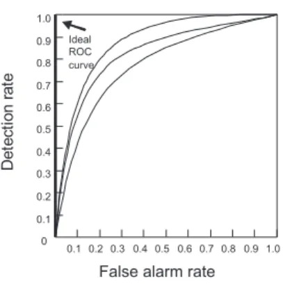
2.4.1 Detection Rate, False Alarm Rate and ROC Curves. The effectiveness of
outlier detection techniques can typically be evaluated depending on how many outliers are correctly identified and also how many normal data are incorrectly
considered as outliers, the latter of which is also known as false alarm rate. The
receiver operating characteristic (ROC) curves [17] shown in a 2-D graph usually is used to represent the trade-off between the detection rate and false alarm rate. Figure 1 illustrates an example of ROC curve. The effectiveness of outlier detection techniques is desired to maintain a high detection rate while keeping the false alarm rate low [1].
2.4.2 Computational Complexity. The efficiency of outlier detection techniques
can be evaluated by the computational cost, which is known as time & space com-plexity. Also, the efficient outlier detection techniques should be scalable to a large and high dimensional data set. In addition, the amount of memory occupation required to execute outlier detection techniques can be viewed as an important performance evaluation metrics.
2.4.3 User-Defined Parameter. User-defined parameters are quite critical to the
performance of outlier detection techniques in terms of effectiveness and efficiency. These parameters are usually used to define the size of local neighborhood of a point or the threshold of similarity measure. However, the choice of appropriate parameters is not really easy. Thus, the minimal use of user-defined parameters can enhance the applicability of outlier detection techniques.
0.1 0.2 0.3 0.4 0.5 0.6 0.7 0.8 0.9 0 0.1 0.2 0.3 0.4 0.5 0.6 0.7 0.8 0.9 1.0 1.0
False alarm rate
D e te c ti o n ra te
ROC curves for different outlier detection techniques
Ideal ROC curve
Fig. 1. ROC Curves for different detection techniques
3. TAXONOMY FRAMEWORK FOR OUTLIER DETECTION TECHNIQUES In this section, we present a comprehensive taxonomy framework for current out-lier detection techniques. Also, we briefly describe each class of outout-lier detection techniques under this taxonomy framework. In addition, a collection of prevalent definitions of outliers are presented with respect to different outlier detection tech-niques.
3.1 Taxonomy Framework
In this paper, we classify non-supervised outlier detection techniques based on the semantics of input data, as shown in Figure 2. Input data can be classified as simple or complex data sets. For the simple data set, outlier detection tech-niques are divided into parametric, semi-parametric and non-parametric methods. Distribution-based, depth-based and graph-based techniques are proposed for para-metric approaches. Clustering-based, distance-based and density-based techniques are proposed for non-parametric approaches. Neural network-based and support vector machine-based techniques are proposed for semi-parametric approaches. On the other hand, for the complex data sets, outlier detection techniques are grouped depending on different types of data sets described in Section 2. Specifically, subspace-based and distance-based techniques are proposed for high dimensional data sets. Graph-based techniques are proposed for mixed-type attributes data sets. Clustering-based and tree-based techniques are proposed for sequence data sets. Graph-based and distribution-based techniques are proposed for spatial data sets. Model-based, graph-based and density-based techniques are proposed for streaming data sets and clustering-based and distribution-based techniques are proposed for spatial-temporal data sets. Supervised and Semi-supervised approaches can also employ some outlier detection techniques addressed in unsupervised approaches, although they initially need to train on pre-labelled data. This topic is outside the scope of this paper.
O u tl ie r D e te c ti o n M e th o d s S im p le D a ta S e t C o m p le x D a ta S e ts S u p e rv is e d P a ra m e tr ic N o n -P a ra m e tr ic N o n -S u p e rv is e d D is tr ib u ti o n -b a s e d S e m i-S u p e rv is e d S e m i-P a ra m e tr ic H ig h D im e n s io n a l D a ta S e t M ix e d -T y p e A tt ri b u te s D a ta S e t S tr e a m in g D a ta S e t S p a ti a l D a ta S e t S p a ti o -T e m p o ra l D a ta S e t S e q u e n c e D a ta S e t S u p p o rt V e c to r M a c h in e -b a s e d D e p th -b a s e d G ra p h -b a s e d N e u ra l N e tw o rk -b a s e d C lu s te ri n g -b a s e d D is ta n c e -b a s e d D e n s it y -b a s e d S u b s p a c e -b a s e d G ra p h -b a s e d T re e -b a s e d D is tr ib u ti o n -b a s e d C lu s te ri n g -b a s e d D is ta n c e -b a s e d D e n s it y -b a s e d M o d e l-b a s e d Fig. 2. T axonom y of outlier detection tec hniques
3.2 Overview of Outlier Detection Methods
Early work in outlier detection was done in the field of statistics.
Distribution-basedmethods assume that the whole data follow astandard statisticaldistribution
model and determine a point as an outlier depending on whether the point deviates significantly from the data model. These methods can fast and effectively identify
outliers on the basis of an appropriate probabilistic data model. Depth-based
meth-ods use the concept of computational geometry and organize data points in layers
in multi-dimensional data spaces. Each data point is assigned adepth and outliers
are those points in the shallow layers with smaller depth values. These methods
avoid the problem of fitting into data distribution. Graph-based methods make
use of a powerful tool data image and map the data into agraph to visualize the
single or multi-dimensional data spaces. Outliers are those points that are present in particular positions of the graph. These methods are suitable to identify outliers in real-valued and categorical data.
Outlier detection also attracts much attention from thedata miningcommunity.
Traditionalclustering-based methods are developed to optimize the process of
clus-tering of data, where outlier detection are only by-products of no interest. The
novel clustering-based outlier detection methods can effectively identify outliers as points that do not belong to clusters of a data set or as clusters that are
signif-icantly smaller than other clusters. Distance-based methods are used to identify
outliers based on the measure of full dimensionaldistance between a point and its
nearest neighbors in a data set. Outliers are points that are distant from the neigh-bors in the data set. These methods do not make any assumptions about the data distribution and have better computational efficiency than depth-based methods,
especially in large data sets. Density-based methods are proposed to take the local
density into account when searching for outliers. These methods can effectively
identify local outliers in data sets with diverse clusters.
In addition, some classification techniques have been applied to outlier detection.
Unsupervised neural networks based methods can autonomously model the
under-lying data distribution and distinguish between the normal and abnormal classes.
Those data points that are notreproducedwell at the output layer are considered as
outliers. These methods effectively identify outliers and automatically reduce the
input features based on the key attributes. Unsupervised support vector machine
based methods can distinguish between the normal and abnormal classes by
map-ping data into the feature space. Those points that are distant from most other
points or are in relatively sparse regions of thefeature spaceare declared as outliers.
These methods effectively identify outliers without pre-labelled data.
Being concerned with the complex data sets, several novel outlier detection
meth-ods have been proposed to deal with data with specific semantic. Subspace-based
methods project the data into a low-dimensional subspace and declare a point as
an outlier if this point lies in an abnormal lower-dimensional projection, where the density of the data is exceptionally lower than the average. These methods reduce the dimensions of data and efficiently identify outliers in high dimensional
data sets. Tree-based methods construct a specifictree as index to decompose data
structure and use an efficient similarity measure for the sequence data to distin-guish outliers from non-outliers. These methods efficiently identify outliers only
by examining nodes near the root of tree. Model-based methods detect outliers by
the construction of a model, which can represent the statistical behavior of data
stream. Outliers are those points that deviate significantly from the learned model. These methods can efficiently deal with the streaming data in an online fashion. 3.3 Prevalent Definitions of Outlier
The definitions of an outlier have been differently introduced by various outlier detection techniques. Being defined differently, they all aim at identifying instances of unusual behavior when compared to the rest majority of observations. As shown in Table I, we present a collection of prevalent definitions of outliers with respect to specific method-based outlier detection techniques. Clearly, there is no universally accepted definition exists.
Table I. Prevalent definitions of outliers. Author Definition
Hawkins [4] Distribution-based outlier: An outlier is an observation, which deviates so much from other observations as to arouse suspicions that it was generated by a different mechanism.
Barnett and Lewis [5]
Distribution-based outlier: An observation (or subset of observations) which appears to be inconsistent with the remainder of that set of data. Rousseeuw
and Leroy [19]
Distribution-based outlier: LetTbe observations from a univariate Nor-mal distributionN(µ,σ)andois a point fromT. Then the Z-score for ois greater than a pre-selected threshold iffois an outlier.
Rousseeuw and Leroy [19]
Depth-based outlier: Depth-based outliers are points in the shallow con-vex hull layers with the lowest depth.
Laurikkala et al. [29]
Graph-based outlier: Outliers are points that are present in particular positions of the graph.
Yu et al. [38], Jiang et al. [39]
Clustering-based outlier: Outliers are points that do not belong to clus-ters of a data set or as clusclus-ters that are significantly smaller than other clusters.
Knorr and Ng [42]
(i)DB(f,D) outlier: An objectoin a data setT is an outlier if at least a fractionf of the objects inT lies at a greater distance thanDfromo. (ii)DB(k,D) outlier: An objectoin a data setT is an outlier if at most k objects inT lie at distance at mostDfromo.
Ramawamay et al. [44]
DBk
noutlier: The topnpoints with the maximum distance to their own kthnearest neighbor are considered as outliers.
Angiulli and Pizzuti [70]
DBk
ω outlier: Given an integer k, the weight ω of a point is defined as the sum or average of the distances separating it from itsk nearest-neighbors. Outliers are those points scoring the largest values of weight. Breunig et al.
[46]
Density-based outlier: Outliers are points that lie in the lower local density with respect to the density of its local neighborhood.
Hu and Sung [50]
Density-based outlier: A point can be considered as an outlier if its own density is relatively lower than its nearby high density pattern cluster, or its own density is relatively higher than its nearby low density pattern regularity.
Hawkins et al. [57]
Neural network based outlier: Points that are not reproduced well at the output layer with high reconstruction error are considered as outliers. Scholkopf et
al. [61]
Support vector machine based outlier: Points that are distant from most other points or are present in relatively sparse regions of the feature space are considered as outliers.
Aggarwal and Yu [64]
Subspace-based outlier: A point is considered to be an outlier if in some lower-dimensional projection it is present in a local region of abnormal low density.
Muthukrishnan et al. [93]
Time series streaming outlier: If the removal of a point from the time sequence results in a sequence that can be represented more briefly than the original one, then the point is an outlier.
Shekhar et al. [82]
Spatial outlier: A spatial outlier is a spatially referenced point whose non-spatial attribute values are significantly different from those of other spatially referenced points in its spatial neighborhood.
Cheng and Li [98]
Spatio-temporal outlier: A spatial-temporal point whose non-spatial at-tribute values are significantly different from those of other spatially and temporally referenced points in its spatial or/and temporal neigh-borhoods is considered as a spatial-temporal outlier.
4. OUTLIER DETECTION TECHNIQUES FOR SIMPLE DATA SET
In this section, we describe method-based outlier detection techniques for the simple data set. Specifically, we summarize main ideas and relevant features of these techniques, and also give a brief evaluation for each outlier detection category. 4.1 Distribution-Based Method
Distribution-based methods, as typical parametric methods, are the earliest
ap-proach to deal with the outlier detection problem. They assume that the whole data follow a statistical distribution (e.g., Normal, Poisson, Binomial) and make use of mathematics knowledge of applied statistics and probability theory to con-struct a data model. They employ statistical tests to determine a point as an outlier depending on whether it deviates significantly from the data model.
94% of Area 94% Confidence Limits 3% 3% 0 P ro b a b ili ty
Fig. 3. An example of distribution of points
Grubbs and Frank [18] initially carry out the test on detecting outliers in a
uni-variate data set. They assume that the whole data follows a standard statistical
t-distribution and aim to identifyone outlier at each iteration. In particular, each
point has it own G value, which is the Grubbes test statistic value and can be calculated based on the sample mean and standard deviation. If the G value of a point is greater than a threshold value, i.e., the upper critical value of the t-distribution, the hypothesis of no outliers is rejected at corresponding significance level. Furthermore, the point is identified as an outlier and immediately eliminated from the data set. The procedure will be repeated until no more outliers are de-tected. The approach does not require user-defined parameters and all parameters are calculated directly from original data. However, multiple iteration may change the probabilities of detection and influence the accuracy of the test.
Three most important fundamental textbooks [4, 5, 19] concerning with outlier detection present classical definitions of distribution-based outliers respectively, as
shown in table (0??). Also, Barnett and Lewis [5] and Rousseeuw and Leroy [19]
further address a comprehensive description and analysis ofstatisticaloutlier
detec-tion techniques. They discuss the problem of detecting outliers inunivariate and
multivariate data. In detecting univariate outliers, they assume that data points
can be modelled by a statistical standard distribution, usually the Gaussian (nor-mal) distribution being used. The statistical distribution includes two parameters, the mean and standard deviation. Based on the observation that the probability
0.0027, thus, three standard deviations is used as a threshold to determine how significantly a point deviates from the data model, as shown in Figure 3.
Alter-natively, a simplified Z-score function that more directly represents the degree of
anomaly of each point is defined as:
Z = (x−µ)/σ (1)
Whereµis the mean,σis the standard deviation. If the absolute value of Z-score
of a data point is greater than 3, the point is declared as an outlier. On the other hand, in detecting multivariate outliers, they usually assume a multivariate normal distribution to represent the data. In order to use a simple threshold to determine
whether a point is an outlier or not, theMahalanobis distance, an effective distance
measure, can take the shape of the multivariate data distribution into account
and identify the attribute correlations accurately. For ad-dimensional multivariate
samplexi (i= 1;n), the Mahalanobis distance is defined as:
M Di =
q
(xi−t)TΣ−1(xi−t) (2)
where Σ represents the d×d covariance matrix and t is the multivariate mean.
Furthermore, forN d-dimensional points from a normal distribution, the square of
Mahalanobis distance follow a chi-square distribution (χ2
d) withddegree of freedom
[20]. Thus, an outlier in multivariate data is a point whose Mahalaobis distance is larger than a pre-defined threshold. Alternatively, Euclidean distance is another basic distance measure and is defined as:
EDi= v u u tXn i=1 (xi−yi)2 (3)
wherexi,yiare two points andn is the dimensionality of the data. The Euclidean
measure is seldom used in distribution-based outlier detection approaches since it cannot effectively capture the shape of the multivariate data distribution. The authors further carry out numerous discordance tests under different circumstances depending on the data distribution, the distribution parameters, the number of expected outlier and the types of expected outlier. The testing results show that the approach achieves good performance in finding outliers in univariate data.
Based on their work, [21, 22] propose robust outlier detection approache based on the minimum covariance determinant (MCD), which aims at alleviating the problem that the mean and standard deviation of the distribution may be extremely sensitive to outliers during the computation of Mahalanobis distance. The main idea of MCD
is to only use asubset of points, which are the minimum number of non-outliers to
minimize the determination of the covariance matrix.
Eskin [23] proposes a mixture model approach to detect outliers in univariate
data. The author assumes that the data is modelled as a mixture of two distribu-tions M and A, which represent the majority of normal points and the minority of anomalous points respectively. Each point in the data set is fallen into either M
or A based on corresponding probability value λ. Initially, all of data points are
put in the set of M while the set of A is empty. The probability function of the entire data may change by moving a data point from M to A. If the difference of
declared as an outlier and then moved permanently to A. The procedure will be repeated until every point in the set of M experiences the comparison. The choice
of two user-defined parametersλandcis very important and may greatly influence
the performance of this approach.
Yamanishi et al. [24] present amixed model of Gaussian distribution to represent
the normal behaviors of data in the detection of outliers. Each data point is assigned a score based on the degree to which the point deviates from the model. A higher score of a point indicates that the point is more likely to be an outlier. This outlier detection approach can be used to handle categorical and continuous variables.
4.1.1 Evaluation of Distributed-based Techniques. Distribution-based approaches
are mathematically justified and can effectively identify outliers if a correct prob-abilistic data model is given. Also, the construction of the data model helps to store minimal amount of information to represent the model, instead of the entire actual data. However, distribution-based techniques suffer from two serious prob-lems. Firstly, these techniques only work well in a single-dimensional data set so that they are not suitable to identify outliers in even moderately high dimensional spaces. Secondly, in many real-life situations, a priori knowledge of data distribu-tion is not available. Finding a possible standard distribudistribu-tion that fits the data is computationally expensive and eventually may not produce satisfactory results. 4.2 Depth-Based Method
Depth-based methods exploit the concept of computational geometry [25] and
or-ganize data points into layers ink-dimensional data space. Based on the definition
ofhalf-space depth [26], also called asdepth contours, each data point is assigned a
depth and outliers are those points in the shallow layers with smaller depth value.
Fig. 4. An example of depth of points [26]
Rousseeuw and Leroy [19] describe two basic depth-based outlier detection
tech-niques for low dimensional data sets, i.e., minimum volume ellipsoid (MVE) and
convex peeling. MVE uses the smallest permissible ellipsoid volume to define a boundary around the majority of data. Those points are outliers if they are not in the densely populated normal boundary. Convex peeling maps data points into con-vex hull layers in data space according to peeling depth. Outliers are those points in the shallow convex hull layers with the lowest depth. Both MVE and convex peeling are robust outlier detection techniques that use the specific percentages of data points to define the boundary. Thus, these outlying points will not skew their
boundary. The key difference between the two techniques is how many outliers are identified at a time. In particular, MVE maintains all data points to define
a normal boundary, then removes multiple outliers at once, while convex peeling
builds convex hull layers and then peels awayone outlier with the lowest depth at
a time. The procedure will be repeated until a pre-defined number of outliers have been removed from the data set.
Based on [19], Ruts and Rousseeuw [27] present an outlier detection approach
using the concept of depth contour to compute the depth of points in a
two-dimensional data set. The deeper the contour a data point fits in, the more robust it is regarded as an outlier. Johnson et al. [28] further extend the work of [27], and
propose a faster outlier detection approach based on computingtwo-dimensional
depth contours in convex hull layers. In particular, this approach only needs to
compute the first k depth contours of a selected subset of points, instead of the
entire data as it is done in [27] and it is robust against collinear points.
4.2.1 Evaluation of Depth-based Techniques. Depth-based approaches avoid the
problem of fitting to a data distribution but instead compute multi-dimensional convex hulls. However, they are inefficient for the large data set with high dimen-sionality, where the convex hull will be harder to discern and is computationally more expensive. Experimental results show that existing depth-based methods provide acceptable performance for only up to 2-dimensional space.
4.3 Graph-Based Method
Graph-based methods make use of a powerful tooldata image, i.e., map the data
into a graph to visualize the single or multi-dimensional data spaces. Outliers are expected to those points that are present in particular positions of the graph.
Laurikkala et al. [29] propose an outlier detection approach for univariate data
based onbox plot, which is a simplesingle-dimensional graphical representation and
includes five number values: lower threshold, low quartile, median, upper quartile and upper threshold. Figure 5 shows an example of a box plot. Using box plot, points that lie outside the lower and upper threshold are identified as outliers. Also, these detected outliers can be ranked by the occurrence frequencies of
out-liers. Thus, the box plot effectively identifies the top n outliers with the highest
occurrence frequencies and then discards these outliers. The approach is applicable for real-valued, ordinal and categorical data. However, it is too subjective due to excessively rely on experts to determine several specific points plotted in the graph, e.g., low and upper quartile.
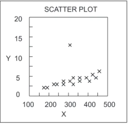
Scatter plot [30] is a graphical technique to detect outliers in two-dimensional
data sets. It reveals a basic linear relationship between the axis X and Y for
most of the data. An outlier is defined as a data point that deviates significantly from a linear model. Figure 6 shows an example of a scatter plot. In addition,
spin plot [31] can be used for detecting outliers in 3-D data sets. D-D plot [22] is
used to illustrate the relationship between a MCD-based robust distances [21] and the full Mahalanobis distances on detecting outliers. Marchette and Solka [32] use
interpoint distance measure to order the data image in data sets to roughly group
100 120 140 160 180 BOX PLOT
X
200
Fig. 5. An example of a box plot
100 200 300 400 500 0 5 10 15 20 SCATTER PLOT X Y
Fig. 6. An example of a scatter plot.
4.3.1 Evaluation of Graph-based Techniques. Graph-based approaches have no
assumptions about the data distribution and instead exploit the graphical repre-sentation to visually highlight the outlying points. They are suitable for identifying outliers in real-valued and categorical data. However, they are limited by the lack of precise criteria to detect outliers. In particular, several specific points in the graph are determined subjectively by experts, which is also a very time-consuming and difficult process.
4.4 Clustering-Based Method
Clustering-base methods use one data mining technique, i.e., clustering, to
effec-tively and efficiently cluster data. Traditional clustering-based approaches, e.g., DBSCAN [33], CHAMELEON [34], BIRCH [35], CURE [36] and TURN [37] are developed to optimize the process of clustering rather than detect outliers. Also, they do not have a formal and acceptive definition for outliers. Thus, detecting outliers in these approaches are only by-products of no interest. Here, we describe several novel outlier detection approaches, which are designed specially for detect-ing outliers based on clusterdetect-ing techniques. In these approaches, outliers are points that do not belong to clusters of a data set [38] or are clusters that are significantly
smaller than other clusters [39]. As shown in Figure 7, the pointsO1, O2 and the
cluster C1 are outliers. The detection of local outliers in clusters is addressed in
[40, 41] .
O1
O2 C1
Fig. 7. An example of clusters of points
Yu et al. [38] propose an outlier detection approach based on a signal-processing
technique wavelet transform, which has the multi-resolution property and can be
extended to detect outliers in data sets with different densities. In particular, this approach uses wavelet transform to quantize the data space and finds the dense clusters in the transformed space. By removing clusters from the original data, the remaining points in the non-dense clusters are labelled as outliers. This approach cannot measure the degree of outlierness, and also do not detect outliers by considering the distance between small clusters and their closest large cluster.
Jiang et al. [39] present atwo-phase clustering approach to identify outliers. In
the first phase, this approach partitions the data into clusters based on aheuristic
instead of the traditional k-means algorithm, which is optimized to search for a
fixed number of clusters. The used heuristic states “if the points in the same cluster are not close enough, the cluster can be split to two smaller clusters”. This helps to reduce the time complexity since the data is processed as fractions and not as whole. In the second phase, this approach employs an outlier-finding process (OFP) to identify outliers based on the construction of a minimum spanning tree (MST), which can remove the longest edge of the tree. Eventually, the small clusters with less number of nodes in the tree are considered as outliers.
He et al. [40] introduce a new definition of a cluster-based local outlier, which
takes both the size of a point’s cluster and the distance between the point and its closest cluster into account. Each point is associated with a cluster-based local outlier factor (CBLOF), which is used to determine the degree of its outlierness.
The proposed approach first partitions the data into clusters by using a squeezer
algorithm, which only makes one scan over the data set and produces good clus-tering results. Then the outlier factor is computed for each point and outliers are points which have the largest values. This approach has the linear scalability with respect to the size of data and can work well in large data sets.
Ren et al. [41] propose a more efficient clustering-based local outlier detection
approach by combining the detection of outliers with grouping data into clusters
process addressed in [38, 39, 40]. The degree of a point’s outlierness is measured by a local connective factor (LCF), which indicates how significantly the point connects with other points in the data set. Specifically, LCF is further calculated by a
vertical data representationP-Tree[41], which uses logical operations to efficiently
compress the data and can be used as an index for the pruning. Outliers are those points that are not connected with clusters. Experimental results show that this approach has better performance in terms of efficiency for large data sets compared to approaches reported in [39, 40].
4.4.1 Evaluation of Clustering-based Techniques. Clustering-based approaches
do not require a priori knowledge of data distribution and exploit clustering tech-niques to efficiently filter and remove outliers in large data sets. In particular, novel clustering-based approaches have been developed to optimize the outlier detection process and reduce the time complexity with respect to the size of data. However, these approaches are suspectable to high dimensional data sets since they rely on the full-dimensional distance measure of points in clusters.
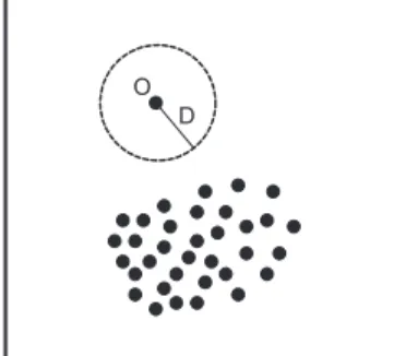
4.5 Distance-Based Method
Distance-based methods, as typicalnon-parametricmethods, identify outliers based
on the measure of full dimensional distance between a point and its nearest neighbor
in the data set. Euclidean distance is commonly used as a similarity measure in
distance-based methods.
D O
Fig. 8. An example of a distance of an outlier
Knorr and Ng [42, 43] define a distance-based outlier as, “a point o in a data set
T is a DB(p,D) outlier if at least a fraction p of the points in T lies at a greater
distance than Dfrom o”. An example of a distance-based outlier is hown in Figure
8. Based on this definition, the detection of outliers relies on Euclidean distance
to measure similarity between every pair of points. The two parameters D and
p are used to determine the range of neighborhood. The authors further propose
threeoutlier detection algorithms, i.e., index-based, nested-loop and cell-based. The
index-based algorithm is based on a priori constructed index structure and executes
a range search with radiusD for each point. If more thanM = (1−p)N neighbors
are found in a point’sD-neighborhood, the search will stop and the point is declared
cost of preliminary construction of the index, and instead partitions the entire set of points into blocks and then directly computes the distance between each pair of
points in the blocks. A point that has less thanM neighbors within the distance
D is declared as an outlier. The two algorithms have the same time complexity of
O(k N2), wherek is the dimensionality andN is the number of points in the data
set. Thecell-based algorithm partitions the entire data set into cells and effectively
prunes away a large number of non-outlier cells before finding out outliers. This helps to speed up outlier detection by only detecting outliers in the subset of cells, which may include potential outliers. These algorithms depend on two user-defined
parameters D and p, which are not usually easy to determine. Also, they do not
provide a ranking on the degree of outliers.
Ramaswamy et al. [44] further extend the outlier definition in [42] based on
the distance of a point from itskth nearest neighbor, instead of the estimation of
an appropriate distance D. Also, they provide a ranking of the top n outliers by
the measure of the outlierness of points. Their novel definition of distance-based
outliers is that the topnpoints with the maximum distance to their ownkthnearest
neighbor are considered as outliers. The authors also exploit the index-based and
nested-loop algorithms to detect outliers. Furthermore, they propose a
partition-based algorithm to prune a significant number of partitions and efficiently identify
the top n outliers in the rest of partitions from the data. Experimental results
show that this partition-based algorithm reduces the cost of computation and I/O in large and multi-dimensional data sets. However, these algorithms suffer from the
choice of the input parameter k. Also they only consider the distance to the kth
nearest neighbor and ignore distance to other closer points.
Bay and Schwabacher [45] propose an optimized nested-loops algorithm that has
near linear time complexity on mining the top n distance-based outliers. They
randomize the data and partition the data into multiple blocks. Each point is associated with an anomaly score, which is determined by either the distance to its
kth nearest neighbor or the average distance to its k nearest neighbors. The top
n distance-based outliers with the largest scores initially are identified in the first
block. Then the smallest score of them is used as acut-off for the rest of blocks.
If a point in other blocks has a larger score than the cut-off, the cut-off will be
increased and replaced by the smallest score in the new n outliers, otherwise, the
point will be pruned. Eventually, n extreme outliers are identified and the cutoff
increases along with pruning efficiency. However, the algorithm is sensitive to the order of data and the distribution of the data set. If the data is sorted or correlated, the performance is poor and time complexity is of quadratic order in the worst case.
4.5.1 Evaluation of Distance-based Techniques. Distance-based approaches do
not make any assumption about the data distribution and are computationally more efficient than the depth-based approaches for large data sets. The proposed distance-based outliers definitions can generalize many notions from distribution-based approaches. However, they rely on the existence of some well-defined notions of distance to measure the similarity between two data points in the entire space, which is not easy to define in high dimensional data sets. Also, they only identify outliers in a global view and are not flexible to discover local outliers, especially in data sets which have diverse densities and arbitrary shapes.
4.6 Density-Based Method
A key problem of distance-based approaches is that they suffer from detecting local outliers in a data set with diverse densities. For example, as shown in Figure 9, two
points O1 and O2 are viewed as outliers with respect to the clusters C1 and C2,
respectively. However,O2may not be an outlier using distance-based methods due
to the fact thatC2 is too dense relative toC1. Thus, density-based approaches are
proposed to solve this problem by takinglocal densityinto account when searching
for outliers. The computation of density still depends on full dimensional distances measure between a point and its nearest neighbors in the data set.
Fig. 9. A problem of distance-based methods in a data set with different densities [46]
Breunig et al. [46] originally introduce the notion of density-based local outliers based on the density in the local neighborhood. Each data point is assigned a local outlier factor (LOF) value, which is calculated by the ratio of the local density
of this point and the local density of its MinPts nearest neighbors. The single
parameter MinPts of a point determines the number of its nearest neighbors in
the local neighborhood. The LOF value indicates the degree of being an outlier depending on how isolated the point is with respect to the density of its local neighborhood. Points that have the largest LOF values are considered as outliers. Based on the work reported in [46], many novel density-based approaches [47, 48, 49, 50, 51, 52, 53] have been developed to further improve the effectiveness and efficiency of LOF. Also, [54] and [55] combine distance-based and density-based approaches to identify outliers in a data set.
Chiu and Fu [47] presentthreeenhancement schemes for LOF calledLOF0,LOF00
andGridLOF. The first two schemes are variants of the original LOF computation
formulation. LOF0 provides a simpler LOF formulation by replacinglocal
reacha-bility density withMinPts-dist, where local reachability density indicates the local
density of a point’s MinPts nearest neighbors, and MinPts-dist indicates the
dis-tance to the point’s MinPts nearest neighbors. This scheme also reduces one scan
over the data on the computation of local reachability density. LOF00is a generation
of LOF by using two differentMinPts values to define a point’s neighborhood and
the point’s neighbors’ neighborhood, and can capture local outliers within
differ-ent circumstances. The third schemeGridLOF uses a simplegrid-based technique
to prune away some non-outliers and then only computes the LOF values for the remaining points. This helps to reduce the computation of LOF for all points,
however, the deletion of points may affect the LOF values of those points in their own neighborhood.
Jin et al. [48] propose an efficient outlier detection approach, which only
de-termines the top n local outliers with the maximal LOF values and reduces the
computation load of LOF in [46] for all points. The approach does not find LOF
values for all points to select the top n outliers, and does not also perform the
process of immediately pruning non-outliers before detecting potential outliers. In-stead, it first uses an efficient clustering technique, i.e., BIRCH [35] to compress the data into micro-clusters, where a group of data is so close together, and then computes LOF upper and lower bounds for each micro-cluster. The micro-clusters
with the largest LOF low bound are chosen to identify the topn local outliers. The
approach suffers from the choice of the parameterMinPts.
Tang et al. [49] present an outlier detection approach more effective than [46],
especially forsparse data sets, where the non-outlier patterns may have low
densi-ties. The approach uses a connectivity-based outlier factor (COF) value to measure the degree of outlierness and takes both the density of the point in its neighborhood and the degree that the point is connected to other points into account. The COF
can be calculated using the ratio of the average distance from the point to its
k-distance neighbors and the average k-distance from itsk-distance neighbors to their
ownk-distance neighbors. Points that have the largest COF values are declared as
outliers.
Hu and Sung [50] consider the problem of detecting outliers in a data set, where
two patterns exist, i.e., high density clustering and low density regularity. The
latter pattern consists of a set of regularly spaced points whose density are lower than that of their neighboring outliers. The authors introduce a new definition of an outlier according to these two different patterns, “if a point’s own density is relatively lower than its nearby high density pattern cluster, or its own density is higher than its nearby low density pattern regularity, the point can be declared
as an outlier”. The definition enhances the effectiveness of LOF, which does not
work well in the low density regularity. The proposed approach uses a variance of volume (VOV) value to measure the degree of being an outlier and has similar time complexity with LOF. Points that have the largest VOV values are declared as outliers. This approach depends on a choice of a parameter constant intensity, which is used to decide the density of clusters.
Papadimitriou et al. [51] present a fast outlier detection approach called LOCI to detect local outliers based on the concept of a multi-granularity deviation factor (MDEF) value, which is used to measure a point’s relative deviation of its local neighborhood density from the average local neighborhood density in its
neighbor-hood. To alleviate the difficulty of choosing values for MinPts in [46, 47], LOCI
uses a different definition for the local neighborhood, where each point has the same radius, instead of the fixed number of neighbors. A point can be declared as an out-lier by comparing its MDEF with a derived statistical value, which is automatically derived from the data. Experimental results show that LOCI achieves good perfor-mance to accurately identify outliers without the user-defined threshold. However, the choice of an appropriate user-defined radius of the local neighborhood becomes a critical issue, especially for high dimensional data sets.
Kim et al. [52] propose an outlier detection approach, which uses the distance
between a data point and its closestprototypesas the degree of outlierness.
Proto-types refer to a small percentage of representative data from the original data can
be identified by using thek-means technique. Then the outlierness of these
proto-types are calculated by taking the measure of distance and density into account. Prototypes with the largest values will be removed. Finally, the approach measures the degree of outlierness of each original data point depending on its distance to its closest remaining prototypes. Outliers are points that are far from their prototypes with the largest distance values. Prototypes are not easily accurately determined, especially in data sets with different densities.
Ren et al. [53] develop an efficient density-based outlier detection approach based on a relative density factor (RDF) value, which is a local density measurement to measure the degree of being an outlier by contrasting the density between a point
and its neighbors. The approach usesP-Treesto efficiently prune some non-outliers,
and then only computes the RDF value for the remaining small subset of the data. Outliers are points whose RDF values are greater than a pre-defined threshold. Experimental results show that the approach has better performance than LOF and LOCI in terms of efficiency for large data sets.
Fan et al. [54] introduce a novel outlier notion by considering bothlocal andglobal
features of the data set. They define an outlier as a point that is inconsistent with the majority of the data or inconsistent with a group of it neighbors. The proposed approach uses a clustering technique, i.e., TURN [26] to efficiently identify outliers by consecutively changing the resolution of a set of data points. The resolution-based outlier factor (ROF) is used to measure the degree of outlierness of a point.
Outliers are the topn points with the lowest ROF values. The approach does not
need any input parameters and is more effective to detect outliers than DB-outlier and LOF.
Kollios et al. [55] propose a density-based biased sampling approach to detect
DB-outlier based onkernel density estimator, which makes use of some randomly
sampled points to represent the density of the whole data set and efficiently approx-imate the underlying probability distribution. Outlier detection can be performed
based on measuring how many points are present within the distanceDfrom a data
point in the data set. After one single-pass through the data, those points that have less number of neighbors in their own neighborhood than a specified threshold are considered as outliers. The performance of this approach depends on the accuracy of the density estimator.
4.6.1 Evaluation of Density-based Techniques. Density-base approaches have no
assumption about the data distribution and effectively identify local outliers in data sets with diverse clusters. However, a weakness of density-based approaches is the determination of input parameters, which are usually based on a priori or trail-and-error estimation. Also, the density definition is based on full dimensional distance computation between points, which is susceptible for high dimensional data sets. 4.7 Neural Network Based Method
Neural networks (NN) are often used in safety-critical applications for regression or classification purpose [56]. They can autonomously model the underlying data
distribution and distinguish the normal/abnormal classes. Recently, unsupervised neural network methods have been applied for outlier detection [56, 57, 58, 59]. Neural networks do not require pre-labelled data to permit learning and can identify those data points that are not reproduced well at the output layer as outliers. The
reconstruction error can be used as the measure of outlierness for data points.
Sykacek [56] presents an outlier detection approach using the equivalent error
bar [56] to identify outliers in the trained network with multi-layer perception.
Outliers are points that are residual outside the equivalent error bar depending on a pre-defined threshold.
Hawkins et al. [57, 58] present an outlier detection approach for large multivariate data sets based on the construction of replicator neural networks (RNN), which is a variant of the usual regression model. Specifically, RNN is a feed-forward multi-layer perception neural network and contains three hidden multi-layers between the input and output layers. Figure 10 shows a schematic view of the fully connected RNN. The use of RNN is to reproduce the input points at the output layer with minimized reconstruction error. If some small number of input points are not reconstructed well and cause high reconstruction errors in the trained neural network, these points can be considered as outliers. An outlier factor is used to measure the degree of outlierness of each point based on the average reconstruction error. Experimental results show that this method is effective for detecting network intrusion.
Fig. 10. Structure of a replicator neural network [57]
Fu and Yu [59] propose an outlier detection approach based on artificial neural network (ANN), which can be trained by different training algorithms. The authors describe three different structures of the trained ANN, i.e., one has no hidden layer, the other two ones have a hidden layer. Outlier detection can be performed in
the three ANNs by a modified Z-score, which is used to measure the degree of
outlierness of data points. If points are statistically inconsistent with the trained neural network, they are declared as outliers.
4.7.1 Evaluation of Neural Network based Techniques. Neural network based
approaches, strictly belong to asemi-parametric method and are trained to model
the underlying data distribution without a priori assumption on the properties of data. They are used to effectively identify outliers and automatically reduce the input features based on the key attributes. However, they are susceptible to


![Fig. 4. An example of depth of points [26]](https://thumb-us.123doks.com/thumbv2/123dok_us/9005623.2386213/15.892.358.565.660.796/fig-example-depth-points.webp)

![Fig. 9. A problem of distance-based methods in a data set with different densities [46]](https://thumb-us.123doks.com/thumbv2/123dok_us/9005623.2386213/21.892.369.549.367.534/fig-problem-distance-based-methods-data-different-densities.webp)
![Fig. 10. Structure of a replicator neural network [57]](https://thumb-us.123doks.com/thumbv2/123dok_us/9005623.2386213/24.892.327.582.574.724/fig-structure-replicator-neural-network.webp)