Vol 2, No 2 (2014)

International Journal of Science Engineering and Advance Technology,

IJSEAT, Vol 2, Issue 2, February - 2014

ISSN 2321-6905

Weighted Contrast Enhancement Based Enhancement For

Remote Sensing Images

Ashok Kumar Dakarapu,V.Anuragh, G Sravan Kumar , Dr.N.S.Murthy Sarma M.TECH Scholar, Assistant Professor, PROFESSOR& head, Dept. of ECE

BVC Engineering college, Odalarevu, AP, India

Abstract

This paper discuss a novel approach based on dominant brightness level analysis and adaptive intensity transformation to enhance the contrast for remote sensing images. In this approach we first perform discrete wavelet (DWT) on the input images and then decompose the bLL sub band into low-, middle-, and high-intensity layers using the log-average luminance. After estimating the intensity transformation, the resulting enhanced image is obtained by using the inverse DWT. The proposed algorithm overcomes this problem using the adaptive intensity transfer function. The experimental results show that the proposed algorithm enhances the overall contrast and visibility of local details better than existing techniques.

Key words- DWT, high intensity layers, bLL.

Introduction

For several decades, remote sensing images have played an important role in many fields such as meteorology, agriculture, geology, education, etc. As the rising demand for high-quality remote sensing images, contrast enhancement techniques are required for better visual perception and color reproduction. Histogram equalization (HE) [1] has been the most popular approach to enhancing the contrast in various application areas such as medical image processing, object tracking, speech recognition, etc. HE-based methods cannot, however, maintain average brightness level, which may result in either under- or oversaturation in the processed image. For overcoming these problems, bi-histogram equalization (BHE) [2] and dualistic sub image HE [3] methods have been proposed by using decomposition of two sub histograms.

For further improvement, the recursive mean-separate HE (RMSHE) [4] method iteratively performs the BHE and produces separately equalized sub histograms.

the dominant brightness level. The adaptive intensity transfer function is computed in three decomposed layers using the dominant brightness level, the knee transfer function [11], and the gamma adjustment

function Then, the adaptive transfer function is applied for color-preserving high-quality

Contrastenhancement. The resulting enhanced image is obtained by the inverse DWT (IDWT).

II. ANALYSIS OF DOMINANT BRIGHTNESS LEVELS

In spite of increasing demand for enhancing remote sensing images, existing histogram-based contrast enhancement methods cannot preserve edge details and exhibit saturation artifact sin low- and high-intensity regions. In this section, we present contrast enhancement algorithm for remote sensing images using dominant brightness level-based adaptive intensity transformation as shown in Fig. 1.If we do not consider spatially varying intensity distributions, the correspondingly contrast-enhanced images may have intensity distortion and lose image details in some regions. For overcoming these problems, we decompose the input image into multiple layers of single dominant brightness levels. To use the low-frequency luminance components, we perform the DWT on the input remote sensing image and then estimate the dominant brightness level using the log-average luminance in the LL sub band [8]. Since

high-intensity values are dominant in the bright region, and vice versa, the dominant brightness at the position (x, y) is computed as

International Journal of Science Engineering and Advance Technology,

IJSEAT, Vol 2, Issue 2, February - 2014

ISSN 2321-6905

III.EDGE PRESERVING CONTRAST ENHANCENT USING ADAPTIVE INTENSITY TRANSFORMATION

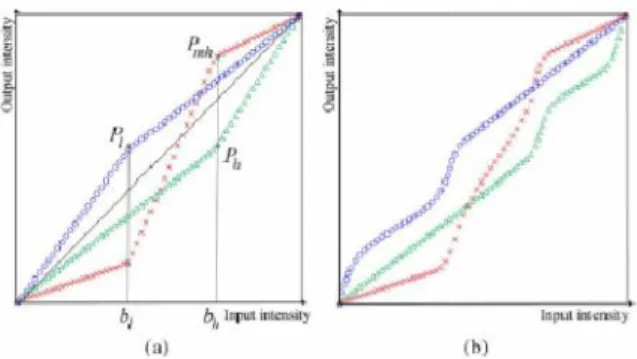
Based on the dominant brightness in each decomposed layer, the adaptive intensity transfer function is generated Since remote sensing images have spatially varying intensity distributions, we estimate the optimal transfer function in each brightness range for adaptive contrast enhancement. The adaptive transfer function is estimated by using the knee transfer[11] and the gamma adjustment functions [12], [13]. For the global contrast enhancement, the knee transfer function stretches the low-intensity range by determining knee points according to the dominant brightness of each layer as shown in Fig. 3(a). More specifically, in the low-intensity layer, a single knee point is computed as

whereblrepresents the low bound,wlrepresents the tuning parameter, and ml represents the mean of brightness in the low intensity layer. For the high-intensity layer, the corresponding knee point is computed as

where bh represents the high bound, wh represents the tuning parameter, and mh represents the mean brightness in the high intensity layer. In the middle-intensity layer, two knee points are computed

where wm represents the tuning parameter and mm represents the mean brightness in the middle-intensity layer. The global image contrast is determined by tuning parameter wi for i

∈

{l,m, h}. Although the contrast is more enhanced as the wi increases, the resulting image is saturated and contains intensity discontinuity. In this letter, we can adjust only the middle-intensity tuning parameterwm for reducing such artifacts. Fig. 3(a) shows knee

transfer functions for three layers using the corresponding knee points and spline interpolation Since the knee transfer function tends to distort image details in the low- and high-intensity layers, additional compensation is performed using the gamma adjustment function. The gamma adjustment function is modified from the original version by scaling and translation to incorporate the knee transfer function as

Since the knee transfer function tends to distort image detail sin the low- and high-intensity layers, additional compensation is performed using the gamma adjustment function. The gamma adjustment function is modified from the original version by scaling and translation to incorporate the knee transfer function as

whereM represents the size of each section intensity range, such asMl=bl,Mm=bh − bl, andMh= 1− bh,L represents the intensity value, andγrepresents the pre specified constant. The pre specified constant γcan be used to adjust the local image contrast. Asγ increases, the resulting image is saturated around bl/2,bh − bl/2, and 1− bh/2. Therefore, theγvalueis selected by computing maximum values of adaptive transfer function in ranges{0 ≤ L <(bl/2)},{bl ≤ L < (bh − bl/2)},and {bh ≤ L < (1 − bh/2)}, which are smaller than bl/2, bh −bl/2, and 1 − bh/2, respectively. The proposed adaptive transfer function is obtained by combining the knee transfer function and the modified gamma adjustment function as shown in Fig. 3(b). Three intensity transformed layers by using the adaptive intensity transfer function are fused to make the resulting contrast-enhanced imagein the wavelet domain. We extract most significant two bits from the low-, middle-, and high-intensity layers for generating the weighting map, and we compute the sum of the two bit values in each layer. We select two weighting maps that have two largest sums. For removing the unnatural borders of fusion, weighting maps are employed with the Gaussian boundary smoothing filter. As a result, the fused imageFis estimated as

WhereW1 represents the largest weighting map, W2 represents the second largest weighting map, cl represents the contrast enhanced brightness in the low-intensity layer, cm represents the contrast-enhanced brightness in the middle-intensity layer, andchrepresents the contrast-enhanced brightness in the high-intensity layer. Since (7) represents the point operation, the pixel coordinate (x, y) is omitted. The fused LL sub band undergoes the IDWT together with the unprocessed HL,LH, and HH sub bands to reconstruct the finally enhanced image.

Fig. 3. (a) Knee transfer functions for three layers using the corresponding knee points and spline interpolation. bl and bh represent low and high bounds ,respectively, of intensity, and_,×, and _ represent low-, middle-, and for evaluating the performance of the proposed algorithm, we tested three low-contrast remote sensing images as shown in Figs. 4–6(a). The performance of the proposed algorithm is compared with existing well-known algorithms including standard HE, RMSHE, GC-CHE, and Demirel’s methods.

For the experiment, we used γ= 1.4, bl = 0.4,

and bh = 0.7. For three different intensity layers,

wl = 1,wm = 3, andwh = 1 were used.

Figs. 4–6 show the results of contrast enhancement using the standard HE, RMSHE, GC-CHE, Demirel’s, and the proposed methods. As shown in Figs. 4–6(b), the results of the standard HE method show under- or oversaturation artifacts because it cannot maintain the average brightness level.

Although RMSHE and GC-CHE methods can

preserve the average brightness level, and better enhance overall image quality, they lost edge details in low- and high-intensity ranges as shown in Figs. 4–6(c) and (d). On the other hand, Demirel’s method could not sufficiently enhance the low-intensity range as shown in Figs. 4–6(e) because of the singular-value con-straint of the target image. Figs. 4–6(f) show the results of the proposed contrast enhancement method. The overall image quality is significantly enhanced with preserving the average brightness level and edge details in all intensity ranges.

For performance evaluation, we used the measure of en-hancement (EME) [15], which is computed

where k₁k_{2 represents the total number of}

blocks in an image, I_max(k, l) represents the

maximum value of the block, Imin(k, l)

represents the minimum value of the block, and c

represents a small constant to avoid dividing by

zero. In this letter, we used 8×8 blocks and c=

0.0001.

EME values for different enhancement methods are listed in Table I. Comparison of EME values show that the proposed method

outperforms existing enhancement methods

TABLE I

EME VALUES OF FIVE

DIFFERENT ENHANCEMENT METHODS WhereW1 represents the largest weighting map,W2

represents the second largest weighting map, cl represents the contrast enhanced brightness in the low-intensity layer, cm represents the contrast-enhanced brightness in the middle-intensity layer, andchrepresents the contrast-enhanced brightness in the high-intensity layer. Since (7) represents the point operation, the pixel coordinate (x, y) is omitted. The fused LL sub band undergoes the IDWT together with the unprocessed HL,LH, and HH sub bands to reconstruct the finally enhanced image.

Fig. 3. (a) Knee transfer functions for three layers using the corresponding knee points and spline interpolation. bl and bh represent low and high bounds ,respectively, of intensity, and_,×, and _ represent low-, middle-, and for evaluating the performance of the proposed algorithm, we tested three low-contrast remote sensing images as shown in Figs. 4–6(a). The performance of the proposed algorithm is compared with existing well-known algorithms including standard HE, RMSHE, GC-CHE, and Demirel’s methods.

For the experiment, we used γ= 1.4, bl = 0.4,

and bh = 0.7. For three different intensity layers,

wl = 1,wm = 3, andwh = 1 were used.

Figs. 4–6 show the results of contrast enhancement using the standard HE, RMSHE, GC-CHE, Demirel’s, and the proposed methods. As shown in Figs. 4–6(b), the results of the standard HE method show under- or oversaturation artifacts because it cannot maintain the average brightness level.

Although RMSHE and GC-CHE methods can

preserve the average brightness level, and better enhance overall image quality, they lost edge details in low- and high-intensity ranges as shown in Figs. 4–6(c) and (d). On the other hand, Demirel’s method could not sufficiently enhance the low-intensity range as shown in Figs. 4–6(e) because of the singular-value con-straint of the target image. Figs. 4–6(f) show the results of the proposed contrast enhancement method. The overall image quality is significantly enhanced with preserving the average brightness level and edge details in all intensity ranges.

For performance evaluation, we used the measure of en-hancement (EME) [15], which is computed

where k₁k_{2 represents the total number of}

blocks in an image, I_max(k, l) represents the

maximum value of the block, Imin(k, l)

represents the minimum value of the block, and c

represents a small constant to avoid dividing by

zero. In this letter, we used 8 ×8 blocks and c =

0.0001.

EME values for different enhancement methods are listed in Table I. Comparison of EME values show that the proposed method

outperforms existing enhancement methods

TABLE I

EME VALUES OF FIVE

DIFFERENT ENHANCEMENT METHODS WhereW1 represents the largest weighting map, W2

represents the second largest weighting map, cl represents the contrast enhanced brightness in the low-intensity layer, cm represents the contrast-enhanced brightness in the middle-intensity layer, andchrepresents the contrast-enhanced brightness in the high-intensity layer. Since (7) represents the point operation, the pixel coordinate (x, y) is omitted. The fused LL sub band undergoes the IDWT together with the unprocessed HL,LH, and HH sub bands to reconstruct the finally enhanced image.

Fig. 3. (a) Knee transfer functions for three layers using the corresponding knee points and spline interpolation. bl and bh represent low and high bounds ,respectively, of intensity, and_,×, and _ represent low-, middle-, and for evaluating the performance of the proposed algorithm, we tested three low-contrast remote sensing images as shown in Figs. 4–6(a). The performance of the proposed algorithm is compared with existing well-known algorithms including standard HE, RMSHE, GC-CHE, and Demirel’s methods.

For the experiment, we used γ= 1.4, bl = 0.4,

and bh = 0.7. For three different intensity layers,

wl = 1,wm = 3, andwh = 1 were used.

Figs. 4–6 show the results of contrast enhancement using the standard HE, RMSHE, GC-CHE, Demirel’s, and the proposed methods. As shown in Figs. 4–6(b), the results of the standard HE method show under- or oversaturation artifacts because it cannot maintain the average brightness level.

Although RMSHE and GC-CHE methods can

preserve the average brightness level, and better enhance overall image quality, they lost edge details in low- and high-intensity ranges as shown in Figs. 4–6(c) and (d). On the other hand, Demirel’s method could not sufficiently enhance the low-intensity range as shown in Figs. 4–6(e) because of the singular-value con-straint of the target image. Figs. 4–6(f) show the results of the proposed contrast enhancement method. The overall image quality is significantly enhanced with preserving the average brightness level and edge details in all intensity ranges.

For performance evaluation, we used the measure of en-hancement (EME) [15], which is computed

where k₁k_{2 represents the total number of}

blocks in an image, I_max(k, l) represents the

maximum value of the block, Imin(k, l)

represents the minimum value of the block, and c

represents a small constant to avoid dividing by

zero. In this letter, we used 8×8 blocks and c=

0.0001.

EME values for different enhancement methods are listed in Table I. Comparison of EME values show that the proposed method

outperforms existing enhancement methods

TABLE I

EME VALUES OF FIVE

International Journal of Science Engineering and Advance Technology,

IJSEAT, Vol 2, Issue 2, February - 2014

ISSN 2321-6905

V. CONCLUSION

This work presented a novel contrast

enhancement method for remote sensing images using dominant brightness analysis and adaptive intensity transformation. All the contrast-enhanced layers are fused with an appropriate smoothing, and the processed LL band undergoes the IDWT together with unprocessed LH, HL, and HH sub bands. The proposed algorithm can effectively enhance the overall quality and visibility of local details better than existing state-of-the-art methods including RMSHE, GC-CHE, and Demirel’s methods.

EXPERIMENTAL RESULTS:

Reference

[1] R. Gonzalez and R. Woods, Digital Image

Processing, 3rd ed.Englewood Cliffs, NJ: Prentice-Hall, 2007.

[2] Y. Kim, “Contrast enhancement using brightness preserving bi-histogram equalization,” IEEE Trans. Consum. Electron., vol. 43, no. 1, pp. 1–8, Feb. 1997.

[3] Y. Wan, Q. Chen, and B. M. Zhang, “Image enhancement based on equal area dualistic sub-image

histogram equalization method,” IEEE Trans.

Consum. Electron., vol. 45, no. 1, pp. 68–75, Feb. 1999.

[4] S. Chen and A. Ramli, “Contrast enhancement using recursive meanseparate histogram equalization for scalable brightness preservation,” IEEE Trans. Consum. Electron., vol. 49, no. 4, pp. 1301–1309, Nov. 2003.

[5] T. Kim and J. Paik, “Adaptive contrast

enhancement using gaincontrollable clipped

histogram equalization,” IEEE Trans. Consum.

Electron., vol. 54, no. 4, pp. 1803–1810, Nov. 2008.

[6] H. Demirel, C. Ozcinar, and G. Anbarjafari, “Satellite image contrast enhancement using discrete

wavelet transform and singular value

decomposition,” IEEE Geosci. Reomte Sens. Lett., vol. 7, no. 2, pp. 3333–337,Apr. 2010.

[7] H. Demirel, G. Anbarjafari, and M. Jahromi, “Image equalization based on singular value

decomposition,” in Proc. 23rd IEEE Int. Symp.

Comput. Inf. Sci., Istanbul, Turkey, Oct. 2008, pp. 1– 5. [8] E. Reinhard, M. Stark, P. Shirley, and J. Ferwerda, Photographic tone reproduction for digital

images,” in Proc. SIGGRAPH Annu. Conf.

Comput.Graph., Jul. 2002, pp. 249–256.

[9] L. Meylan and S. Susstrunk, “High dynamic range image rendering with a retinex-based adaptive filter,” IEEE Trans. Image Process., vol. 15, no. 9, pp. 2820–2830, Sep. 2006.

[10] S. Chen and A. Beghdadi, “Nature rendering of color image based on retinex,” in Proc. IEEE Int.

Conf. Image Process., Nov. 2009, pp. 1813–1816.