Vol 10, No 1 (2018)

New Holes and Boundary Detection Algorithm for

Heterogeneous Wireless Sensor Networks

Ahmed M. Khedr

and Arwa Attia

1

Computer Science Department, University of Sharjah, Sharjah 27272, UAE

1,2

Mathematics Department, Zagazig University, Zagazig, Egypt.

Abstract: Hole is an area in wireless sensor network (WSN) around which nodes cease to sense or communicate due to drainage of battery or any fault, either temporary or permanent. Holes impair sensing and communication functions of network; thus their identification is a major concern. In this paper, a distributed solution is proposed for detecting boundaries and holes in the WSN using only the nodes connectivity information and estimated distance between nodes. Our protocol is divided into four main phases. In the first phase, each node discovers its coverage neighbors and collects their information. In the second phase, each node communicates with its neighbors to find whether its sensing range is fully covered by the sensing ranges of its neighbors. In the third phase, the boundary nodes connect with each other to complete the boundary information. In the fourth phase, a boundary sub-graph amongst boundary nodes is constructed and classified either as an interior or an exterior boundary. Simulation results show that our approach improves the energy and reduces the number of boundary nodes over existing algorithms.

Keywords: Arbitrary sensing ranges, Coverage holes, Boundary detection, Distributed algorithm, Un-localized sensors.

1.

Introduction

WSN is a network composed of a large number of nodes by means of self-organization and multi-hops. WSNs have myriad of interdisciplinary applications such as weather forecasting, battlefield surveillance, threat identification, health monitoring and environment monitoring [1, 14]. All those applications that demand random deployment and uncontrolled environment suffer from holes problem. Hole detection is one of the major problems in WSN. Holes affect the network capacity and perceptual coverage of the network. Due to limited battery the nodes may die with passage of time. In case of random deployment, there is a huge possibility that all areas of target region are not covered properly leading to formation of holes. Detection of holes is important because of their negative and damaging effects. If there is a hole in the network then data will be routed along the hole boundary nodes again and again which will lead to premature exhaustion of energy present at these nodes. This will ultimately increase the size of hole in the network. Detection of holes avoids the additional energy consumption around holes because of congestion. We detect the hole in WSNs through detection of hole boundary, that is, the nodes that are present on the hole boundary. Whether a node is an inner or a boundary might be crucial for object tracking scenarios. For example, when tracking events entering and leaving a region, boundary nodes might be involved in more complex sensing tasks whereas inner nodes might spend more energy on satisfying routing tasks. Most applications and research works focus on homogeneous WSNs, where all nodes are identical in terms of energy resources, computation and wireless communication capabilities. However, the assumptions that all the nodes have the same sensing or

communication ranges might not be accurate. To overcome these problems, heterogeneous WSNs consisting of two or more different types of nodes: the high-end ones have higher processing throughput and longer communication / sensing range; the low-end ones are much cheaper and with limited computation and communication / sensing abilities. A mixed deployment of these nodes can achieve a balance of performance and cost of a WSN. Numerous real life examples using a large scale WSN use heterogeneous nodes. In this paper, using only estimated distance between nodes, 1- and 2-hops, we present a scalable solution that recognizes both the inner and boundary nodes in a two-dimensional space with heterogeneous sensing range. Our approach sets no constraints on the node distribution and the node density. In addition, we propose two distributed algorithms to characterize some global properties of the boundaries. The rest of the paper is organized as follows: In Section 2, we describe the related work of our problem. The problem assumption, definitions and the proposed algorithm with a step by step description is given in Section 3. The simulation of our algorithm is presented in Section 4. Section 5 concludes our work.

2.

Related Work

[18] is centrality index, where high value is assigned to inner nodes and less value to outer nodes. We have considered many algorithms under different categories each having its own limitations. Geometrical approach for hole detection requires GPS enabled sensors and is expensive. They consume a lot of energy and it is not practical for sensors to know their exact location in hostile environment. Considering huge applications of WSN, these approaches have limited scope. Statistical approaches provide optimal performance, but they are computationally expensive. Owing to the challenges in wireless sensor networks it is not desirable that nodes perform complex mathematical and statistical calculations [15]. Topological approach provides realistic results but involves communication overhead. Some of the algorithms do not work for small network degrees. Topological Approach: Also called as connectivity based approach, it uses only the available connectivity information of network to detect holes. This approach requires no location information and works even for dense networks. There is no assumption about node distribution. One of the algorithms based on topological approach to detect coverage holes within WSNs was given in [19] and later improved in [20]. Authors proposed a distributed cooperative scheme based on the fact that nodes at the hole or network boundary have smaller degrees than interior nodes. It deals with static, uniformly distributed nodes with each node having a unique id. If the degree of a node is lower than the average degree of its 2-hop neighbors, then it makes a decision whether it is on hole boundary or not. If yes, then it sends messages informing its status to its 1-hop neighbors who may also be on hole boundary. The algorithm is scalable, but approach produces poor results for randomly deployed dense networks. If there are not sufficient nodes surrounding a hole then output produced is not accurate. In [21], the authors used the concepts of Rips complex and Cech complex to discover coverage holes. If communication radius is greater than or equal to twice the sensing radius and there is a hole in Rips complex, then there must be a hole in Cech complex. The distributed algorithm proposed by authors is capable of detecting non triangular holes and the area of triangular holes. After constructing neighbor graph, each node checks whether there exists a Hamiltonian cycle in graph. If not, then node is on the hole boundary. After making decision, each node broadcasts its status to its neighbors. The algorithm further finds cycles bounding holes. In [22], the authors proposed a hop based approach to find holes in sensor networks. There are three phases, namely, information collection phase where each node exchanges information to build a list of x-hop neighbors, path construction phase where communication links between sensor nodes in list of x-hop neighbors are identified, and finally path checking phase where paths are examined to infer boundary and inner nodes. If the communication path of x-hop neighbors of a node is broken, then it is a boundary node. Algorithm works for node degree of 7 or higher which is better than some of the other approaches, but there is a huge communication overhead involved identifying x-hop neighbors. In [23], the authors proposed decentralized boundary detection (DBD) algorithm to identify sensor nodes near a hole or obstacle in WSN using topological approach. Each node knows its three-hop neighbors by exchanging HELLO messages and 1-hop and 2-1-hop node information. There is no UDG constraint. Each node then constructs 2-hop neighbor graph. If cycle exists in such a graph, then there is a hole in

network. For dealing with hole which is not included totally inside 2-hop neighbor graph, another rule based on contour structure was developed. Detection of broken contour line implies either network boundary or an obstacle. There are very few algorithms that can detect boundaries of small holes. In [24], the authors proposed a distributed algorithm that can accurately detect boundaries of small holes in the network. The first step of algorithm is to reduce the connectivity graph by using vertex deletion and edge deletion so as to obtain a skeleton graph. Thereafter, skeleton graph is further partitioned to get coarse inner boundary cycles. Each cycle either encloses a hole of graph or corresponds to outer boundary. The coarse outer boundaries are then further refined to get _ne grained boundary cycles. There is no assumption related to node density. The authors further proved the correctness of hole detection.

Our proposed algorithm belongs to the third category where, without network synchronization and position information and using only 1- and 2-hops, we present a scalable algorithm that recognizes both the inner and boundary nodes in a two-dimensional space with heterogeneous sensing range. Our approach sets no constraints on the node distribution and the node density. It uses unit disk graph for the communication range. The proposed algorithm not only reduces the consumed energy but also minimizes the number of nodes that cover the network boundary. Our algorithm can precisely identify the boundary nodes, even in a sparsely deployed environment. The local boundary classifications are used to create a boundary sub-graph and to determine if a boundary sensor node is located on a hole or on the outer boundary of the network.

3.

Boundary and Hole Detection Algorithm

3.1 Problem Assumptions

Our approach relies on the following key assumptions regarding the field and the nodes:

 All sensor nodes are randomly deployed in a monitoring region and some irregular holes may exist.

 Each sensor node has a unique ID.

 The sensor nodes have sensing ranges that are different from their communication ranges

 Every sensor node can estimate the distances from its 1-hop neighbors using RSSI.

3.2 Definitions and Notations

We assume that there are randomly scattered heterogeneous sensor nodes over a monitored area form the set , where such that .

Definition 1: A node is a boundary node if there is a point

p on the sensing region of such that is not covered by the sensing range of any other node.

Definition 2: The shared edge between and where

is the cross edge between the intersection of

and . The shared edges of node is the set of

all shared edges between and the nodes of coverage neighbor = { : where is a shared edge between and a node in }.

Definition 3: A coverage polygon of a node is the

in . is bounded if the number of shared edges equals to the number of vertices.

Here, we outline our proposed algorithm for discovering the hole and its boundary of an un-localized heterogeneous WSN.

The algorithm includes four phases: initial, discovery and detection, selection and connection, and classification. In the first initial phase, each node discovers its coverage neighbors and collects their information. In the second discovery and detection phase, each node communicates with its neighbors to find whether its sensing range is fully covered by the sensing ranges of its neighbors. In the selection and connection phase, the boundary nodes connect with each other to complete the boundary information. In the classification phase, a boundary sub-graph amongst boundary nodes is constructed and classified either as an interior or an exterior boundary.

Here in the following phases, we use two relevant procedures: (1) 1-hop sorting to sort the 1-hop neighbors of a node according to a randomly selected neighbor and (2) 2-hops Distance to characterize connectivity pattern by computing the distance between a node and any other node in its 2-hops neighbors [5].

3.3 Initial Phase: Boundary Coverage Neighbors

Discovery

Lemma: The sensing range of any node can be completely

covered by its and .

Proof: Assume that a sensor node is covered by a sensor

node and i.e., and If and x have maximum sensing range, i.e., , then

and so which induces a

contradiction that implies the sensing range of does not intersect with the sensing range of

In this phase, each node discovers its coverage neighbors and collects their information [5].

3.4 Boundary detection phase

In this phase, every node uses its set to detect if it is a boundary or an inner node in the network by executing the following procedure:

1. If your sensing range is fully covered by one node, then declare yourself as an inner node.

2. Otherwise, using a subset of

construct (we use only a subset of

to reduce the computation complexity of high density networks). The selection of Sub-Neigh(v) will be as follows:

Case 1: select four nodes in four different directions

to construct Sub-Neigh (v) as follows:

 Select a random node and add to

 For each node do

1. Select , such that and

add w to Sub-Neigh ( ).

2. Select , such that and add x to

3. Select , such that and add y to

If cannot create in case 1, it will try one of the following two cases.

Case 2: select 3 nodes in three different directions using

previous procedure.

Case 3: select two nodes in two different directions using

previous procedure and then select cross node between them such that the angle between the cross node and every selected node should be more than or equal to 45o.

3. Using construct by constructing

4. Run the Bounded Test to check the boundedness of the constructed

a. If every two adjacent shared edges in are intersected, then is bounded and therefore, start the covered test.

b. Otherwise, while unbounded or there is an unselected node in .

i. Find a new node in that is close to the unbounded area of (between the two adjacent nodes that do not have shared edge). ii. Add the new selected node to

then reconstruct a

new based on the new

and check the boundedness

of the new .

c. If bounded start the covered test. d. Otherwise, declare yourself as a boundary

node.

Note that the bounded test is not enough to decide the inner nodes because some nodes can pass the bounded test although they are not inner nodes.

Lemma: Every node is a boundary node, if it has

unbounded

Proof: obvious from the bounded test definition.

In the next step, we study the coverage test to decide if the nodes with bounded are inner or boundary nodes.

5. Run Coverage Test: Every node has bounded

and will execute the coverage test as follows: If the vertices of are covered by the sensing range of (covered , declare yourself as an inner node.

Otherwise, for every uncovered vertex execute the following procedure:

a. while there is uncovered vertex and there is no more node in to be selected, do

i. Find node such that w is close to v, and located between the two nodes say p, q that failed to form a covered vertex

ii. Add to and construct the new

iii. If the new is covered, check the next uncovered vertex of iv. Otherwise, delete w from

and find another node in

b. If still there are uncovered vertices of do the following:

i. while there is uncovered or there is unselected node in do

A. Increase the width around v by finding node in such that located between two nodes and and is the previous node to and is the next node to in

and

intersects with and or, with and

B. If there is satisfies the previous conditions, add to

C. Otherwise, select two nodes from such that they are located between and and satisfy the following conditions:

 The sensing ranges of the two selected nodes are intersected.

 The sensing range of r intersects with the sensing range of one of the two selected nodes and the sensing range of s intersects with the other node.

D. Check the new constructed c. If all vertices of are covered, declare

yourself as an inner node. Otherwise, declare yourself as a boundary node.

Lemma: If a node has uncovered , then is a

boundary node.

Proof: Assume that is not fully covered by the

sensing range of , i.e., there exists such that i.e., there is an arc of which is not covered by the sensing ranges of the nodes forming . Therefore, is not fully covered by its boundary coverage neighbors.

In the boundary detection phase, each node directly declares itself as a boundary if its is unbounded or bounded but uncovered by its neighbors. The boundary node announces its decision to its neighbors and then runs the Selection phase, where each boundary node will be connected with two boundary nodes in two different directions to complete its boundary information.

3.5 Selection and Connection Phase

Every boundary node may receive several boundary declaration messages from its neighbor boundary nodes to complete its boundary neighbors list by executing the following procedure:

 Broadcast Boundary Query message to your neighbors with your ID.

 If you receive Boundary Answer messages from your neighbors, select the node with the largest sensing range and smallest vertical distance, and

send Candidate-Node a reply message to be the new selected boundary node.

 Any node that receives a Boundary Query

message from will execute the following

procedure:

 From your neighbor list, find a boundary node w such that w and are located in two different directions, i.e., and

 Send Boundary Answer message containing (your ID, ID of the selected boundary node) to , and then wait for Candidate Node

message reply.

After executing the selection phase, every boundary node will have at least two boundary nodes in its boundary neighbor list. Then, will start the connection phase by executing the following procedure:

 If the following conditions are satisfied:

 for any two boundary nodes and ,

and and,

 there is an overlap between the sensing range of and the sensing ranges of and

 Then, consider and as your forward boundary nodes, otherwise, go back to the selection phase.

3.6 Classification Phase

After each boundary node determines its boundary neighbors list, it uses a broadcast tree leader-election algorithm [27], but with the scope of the messages limited to only boundary nodes. The boundary node in the boundary sub-graph with the lowest ID becomes the root, and this ID is transmitted to all the other boundary nodes in the same boundary sub-graph. Each boundary node (child) in the sub-graph sends its vertical distance to its parent towards the root. Every boundary node will have one of the following two cases: Receiving only one root.ID message

If the received root.ID > is your root.ID, then broadcast (your ID, root.ID) to your boundary node neighbors.

Otherwise, update your root.ID, and send (your ID, root.ID) to your boundary nodes that are not members of your boundary sub-graph (children).

Receiving more than one root.ID message If all messages contain the same root.ID, You are the end node of a boundary sub-graph.

Send (your ID, distance between you and your parents, root.ID) to your parents.

Otherwise, if all messages contain different root IDs and you are the end node of a boundary sub-graph,

You are a member in more than one sub-graph.

Update the root.ID to the smallest one of the received messages, and send (your ID, root.ID) to your boundary nodes (children) that are not members of your boundary sub-graph.

determines if there is a hole inside the network or it actually represents the outer boundary of the network. The root of the graph then rebroadcasts the results back to the sub-graph.

4.

Simulation Results

A simulator has been implemented using ns-2 to estimate the performance of our proposed boundary nodes detection algorithm. Sensor nodes are randomly deployed in the monitoring region. The average node degree of the network is varied from 6 and 23 with an incremental step 4 by changing the sensing radius. The sensing ranges of sensor nodes are heterogeneous and increase with the average node degree of the network. In order to study the performance of our approach, we considered the following performance metrics:

Number of Boundary Nodes: is the number of boundary nodes in the network.

Communication Overhead: is measured by the total number of messages used in discovering boundary sensor nodes and connecting them in sub-graphs.

Energy Consumption: is measured by the total consumed energy in discovering boundary sensor nodes and connecting them in sub-graphs.

Figure 1. Number of boundary nodes under faulty distances

vs. average node degrees.

In the first test, we consider the number of boundary nodes according to three different measurements: the true distance, the 10% faulty distance, and the 30% faulty distance. As expected, Figure 1a shows that the results of faulty distance are not as good as the true distance, especially in low average degree. This is because every sensor node in the network of our algorithm depends on its coverage sensor node set to detect if it’s a boundary or an inner node. Therefore, with existing false distances between the nodes, the coverage set becomes incomplete, which causes many inner nodes to declare themselves as boundary nodes. Note that increasing the average node degree, implies that the boundary nodes remain the same under the three different distances.

The reason is that with good average node degree, the coverage set of each sensor node will be adequate to provide a true declaration. The performance of our algorithm is not affected by the faulty distances among connected sensor nodes and the classification phase.

In the second test, we evaluate the communication overhead of the proposed algorithm as each boundary sensor node exchanges messages with its neighbor nodes to detect its

boundary neighbors or to select new nodes to be new boundary neighbors.

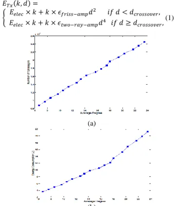
Figure 2a illustrates that the number of exchanged messages increases as the average node degree increases. In order to measure the energy dissipation of nodes, we use the same energy parameters and radio model as discussed in [26], which indicates that the transmission energy consumption is:

(1)

(a)

(b)

Figure 2. (a) Exchanged messages vs. average node degree,

(b) Energy consumption vs. average node degree. The reception energy consumption is

(2)

Where is the energy consumed for the radio electronics, and for a power amplifier. Radio

parameters are set as

, ,

. Figure 2b shows the relation between the

average node degree and the energy consumption. Note that increasing the average degree sensor node causes increase in energy consumption of the network because when the average degree of sensor nodes increases, the number of exchanged messages increases which increases the energy consumption.

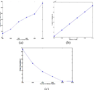
messages increases by increasing the number of deployed sensor nodes. There is a disconnection in the network, the combination process cannot connect these nodes that are on the perimeters of the cycles which leads to classify these nodes as boundary node.

(a) (b)

(c)

Figure 3. (a)Number of boundary nodes vs. number of

deployed nodes in the network, (b)Number of exchanged messages vs. number of deployed nodes in the network, (c) Energy consumption vs. the number of deployed nodes in the network.

Figure 3c shows the energy consumption as the density of the network increases. The results show that the increase in the network density with fixed average degree leads to decrease in the energy consumption because the communication range of the sensor nodes decreases by increasing the density of the network. In summary, the boundary detection approach can identify all the boundary nodes of the network at low average node degree of 6.6 and high density of the network and can connect all the boundary nodes into sub-graphs and correctly classify each Sub-graph as an interior or exterior boundary of the network.

In the fourth test, we compare the simulation results of the proposed algorithm with existing BR algorithm [25]. 3500 sensor nodes are randomly deployed in monitoring regions of 400 m × 400 m and the average node degree is varied from 6 to 16 degree with an increment of 1.

Figure 4a shows the number of boundary nodes in BR and proposed algorithm. It shows that the number of boundary nodes decreases by increasing the average degree. In low average degree, the number of detected boundary nodes using our approach is smaller than the number of boundary nodes in BR because in our approach, each sensor node makes its decision locally and connects itself with the nearby boundary nodes if it detects that it represents a boundary node. While BR detects the boundary nodes by finding the chord-less cycles and then constructs the valid patterns by combining these cycles. Therefore, when there is a disconnection in the network, the combination process cannot connect these nodes that are on the perimeters of the cycles which lead to classify these nodes as boundary nodes.

In Figure 4b, the number of exchanged messages in BR is much bigger than the number of exchanged messages in our proposed algorithm because in BR, the number of exchanged messages between nodes to gather data and construct the valid patterns phase is very large.

However, in our algorithm, the sensor node in WSN makes its decision locally and only needs to exchange messages with its neighbors to decide. Also, in the connection phase of our algorithm, the sensor node exchanges about 3 messages with its boundary nodes to connect itself in the boundary sub-graphs.

(a) (b)

(c)

Figure 4. (a)Number of boundary nodes in BR and the

proposed algorithms with different average node degrees, (b) Exchanged messages in BR and our proposed algorithms, (c) Energy dissipation in BR and our proposed algorithms. Figure 4c shows the energy consumption in BR and the proposed approach. Since the number of exchanged messages in BR algorithm is much larger than the number of exchanged messages in the proposed approach this makes the consumed energy in BR much more than the consumed energy in the proposed approach. We can note that the energy dissipation at an average degree of 10.5 using our algorithm is only 4 J, while it is 180 J in BR.

In summary, our approach can detect the boundary nodes in low average node degree of 6.6 and connect them into different sub-graphs. The number of exchanged messages and consumed energy in our approach is much smaller than exchanged messages and consumed energy in BR.

5.

Conclusion

reduces the number of boundary nodes over existing algorithms.

References

[1] F. Frattolillo, "A Deterministic algorithm for the deployment of wireless sensor networks", International Journal of Communication Networks and Information Security, vol. 8, No. 1, pp. 1-10, 2016.

[2] B. O. Yenke, D. W. Sambo, A. Ari and A. Gueroui, "MMEDD: Multithreading model for an efficient data delivery in wireless sensor networks," International Journal of Communication Networks and Information Security, vol. 8, No. 3, pp. 179- 186, 2016.

[3] C. Titouna1, M. Gueroui, M. Aliouat, A. Ari and A. Amine, "Distributed fault-tolerant algorithm for wireless sensor network," International Journal of Communication Networks and Information Security, vol. 9, No. 2, pp. 241-246, 2017. [4] D. M. Omar, A. M. Khedr and and Dharma P. Agrawal,

“Optimized clustering protocol for balancing energy in wireless sensor networks," Management and Information Technology, pp. 115-124, 2016.

[5] A. M. Khedr, “Location-free minimum boundary coverage in a wireless sensor network," Procedia Computer Science vol. 65, pp. 48-57, 2015.

[6] A. M. Khedr, “Effective data acquisition protocol for multi-hop heterogeneous wireless sensor networks using compressive sensing," Algorithms, vol. 8, No. 4, pp. 910-928, 2015.

[7] A. Salim, W. Osamy, and A. M. Khedr, “IBLEACH: Effective LEACH protocol forwireless sensor networks," Wireless networks, Wireless Networks, vol. 20, pp. 1515-1525, 2014. [8] A. M. Khedr and W. Osamy, “Minimum connected cover of

query regions in heterogeneous wireless sensor networks," Information Sciences, vol. 223, pp. 153-163, 2013.

[9] A. M. Khedr and W. Osamy, “Mobility-assisted minimum connected cover in a wireless sensor network," J. Parallel Distrib. Comput. vol. 72, pp. 827-837, 2012.

[10]A. M. Khedr and W. Osamy, “Effective target tracking mechanism in a self-Organizing wireless sensor network," Journal of Parallel and Distributed Computing, vol. 71, pp.1318-1326, 2011.

[11]A. M. Khedr and W. Osamy, “Minimum perimeter coverage of query regions in heterogeneous wireless sensor networks," Information Sciences, vol. 181, pp. 3130-3142, 2011. [12]A. M. Khedr and W. Osamy, “Finding perimeter of query

regions in heterogeneous wireless sensor networks," Computing and Informatics, vol. 29, no. 4, pp. 1001-1021, 2010.

[13]A. M. Khedr and W. Osamy, and Dhrama P. Agrawal, “Perimeter discovery in wireless sensor networks," J. Parallel Distrib. Comput., vol. 69, pp. 922-929, 2009.

[14]A. M. Khedr, “New mechanism for tracking a mobile target using grid sensor networks," Computing and Informatics, vol. 28, pp.1001-1021, 2008.

[15]I. Khan, H. Mokhtar, and M. Merabti, “A survey of boundary detection algorithms for sensor networks,? in Proceedings of the 9th Annual Postgraduate Symposium on the Convergence of Telecommunications, Networking and Broadcasting, 2008. [16]B. Hofmann-Wellenhof, H. Lichtenegger, and J. Collins,

“Global positioning systems: theory and practice," Springer, Berlin, Germany, 5th edition, 2001.

[17]J. Yang and Z. Fei, “HDAR: Hole detection and adaptive geographic routing for ad hoc networks,” in Proceedings of the 19th International Conference on Computer Communications and Networks (ICCCN ?10), pp. 1-6, August 2010.

[18]S. Fekete, A. Kroller, D. P_sterer, S. Fischer, and C. Buschmann, “Neighborhood-based topology recognition in sensor networks," in Proceedings of Algorithmic Aspects of Wireless SensorNetworks (ALGOSENSORS ?04), vol. 3121

of Lecture Notes in Computer Science, pp. 123-136, Springer, 2004.

[19]B. Kun, G. Naijre, T. Kun, and D.Wanlllo, “Neighborhoodbased distributed topological hole detection," in Proceedings of the IET International Conference on Wireless, Mobile and Multimedia Networks (ICWMMN ?06), pp. 1-4, Hangzhou, China, 2006.

[20]K. Bi, K. Tu, N. Gu, and W.Dong, “Topological hole detection in sensor networks with cooperative neighbors,” in Proceedings of the International Conference on Systems, DOI: 10.1109/ICSNC.2006.71, pp. 131, October 2006. [21]P. Martins, F. Yan, and L. Decreusefond, “Connectivitybased

distributed coverage hole detection in wireless sensor networks," in IEEE Global Telecommunications Conference (GLOBECOM ?11), pp. 1-6, 2011.

[22]S. Zeadally, N. Jabeur, and I. M. Khan, “Hop-based approach for holes and boundary detection in wireless sensor networks," IET Wireless Sensor Systems, vol. 2, no. 4, pp. 328-337, 2012.

[23]W-C. Chu and K.-F. Ssu, “Location free boundary recognition in mobile wireless sensor networks with a distributed approach," ScienceDirect ComputerNetwork, vol. 70, pp. 96-112, 2014.

[24]D. Dong, Y. Liu, and X. Liao, “Fine-grained boundary recognition in wireless ad hoc and sensor networks by topological methods," in Proceedings of the 10th ACM International Symposium on Mobile Ad Hoc Networking and Computing, pp. 135-144, 2009.

[25]O. Saukh, R. Sauter, M. Gauger and P. J. N. Marron, “On boundary recognition without Location Information in wireless sensor networks," ACM Transactions on Sensor Networks (TOSN), vol. 6, No.3, pp.1-35, 2010.

[26]W. Heinzelman, Application-Specific Protocol Architectures for Wireless Networks," PhD thesis, MIT, June 2000. [27]J. McLurkin, “Stupid robot tricks: A Behavior-based