Cite this:DOI: 10.1039/c6sm02252a
Combining cell-based hydrodynamics with hybrid
particle-field simulations: efficient and realistic
simulation of structuring dynamics
G. J. A. Sevink,*aF. Schmid,bT. Kawakatsucand G. Milanod
We have extended an existing hybrid MD-SCF simulation technique that employs a coarsening step to enhance the computational efficiency of evaluating non-bonded particle interactions. This technique is conceptually equivalent to the single chain in mean-field (SCMF) method in polymer physics, in the sense that non-bonded interactions are derived from the non-ideal chemical potential in self-consistent field (SCF) theory, after a particle-to-field projection. In contrast to SCMF, however, MD-SCF evolves particle coordinates by the usual Newton’s equation of motion. Since collisions are seriously affected by the softening of non-bonded interactions that originates from their evaluation at the coarser continuum level, we have devised a way to reinsert the effect of collisions on the structural evolution. Merging MD-SCF with multi-particle collision dynamics (MPCD), we mimic particle collisions at the level of computational cells and at the same time properly account for the momentum transfer that is important for a realistic system evolution. The resulting hybrid MD-SCF/MPCD method was validated for a particular coarse-grained model of phospholipids in aqueous solution, against reference full-particle simulations and the original MD-SCF model. We additionally implemented and tested an alternative and more isotropic finite difference gradient. Our results show that efficiency is improved by merging MD-SCF with MPCD, as properly accounting for hydrodynamic interactions considerably speeds up the phase separation dynamics, with negligible additional computational costs compared to efficient MD-SCF. This new method enables realistic simulations of large-scale systems that are needed to investigate the applications of self-assembled structures of lipids in nanotechnologies.
Introduction
Shared amongst many processes in chemistry and biology is the property that the emergent (deterministic) behaviour associated with basic observable functionality is deeply rooted in a fluctuating network of interactions that are active on many lower microscopic levels, sometimes down to electronic states. Ideally, one should thus pursue a holistic (experimental or computational) multi-scale approach to reach the truly fundamental understanding that is needed for the progress of knowledge,i.e.an approach in which all relevant scales are observed or accounted for realistically and simultaneously, and on an equal footing. The key dilemma in computational modelling, however, is that system size (either in space or time) is inversely proportional to the number of
degrees of freedom in the representation, meaning that the maximum size is fixed by the chosen resolution. Any realistic computational investigation of a multi-scale phenomenon should thus make an inspired choice to sacrifice either one of them to some extent.
Historically, the community studying emergent behaviour in heterogeneous biological/chemical systems has valued resolu-tion over size, and primarily relied on classical molecular simulation. The class of models to which classical all-atom molecular dynamics (AA-MD) belongs – known as particle-based simulations – has the benefit that chemical detail directly translates into specific molecular fragments, atoms in AA-MD1,2 or small groups of (heavy) atoms in coarse-grained MD (CGMD)3and dissipative particle dynamics (DPD),4all in full agreement with standard concepts in chemical research. Nevertheless, the necessity of calculating pair interactions for each small (femtosecond) time steps, required for stable numerical integration of the equations of motion, remains a serious restriction for the upper scales of any trajectory in terms of absolute time and length scales. Particle-based approaches that go beyond the mild coarsening employed in CGMD/DPD aLeiden Institute of Chemistry, Leiden University, P.O. Box 9502, 2300 RA Leiden,
The Netherlands. E-mail: [email protected]
bInstitut for Physik, Johannes Gutenberg Univeristat Mainz, Staudingerweg 7-9, 55128 Mainz, Germany
cDepartment of Physics, Tohoku University, Aoba, Aoba-ku, Sendai 980-8578, Japan dDipartimento di Chimica e Biologia, Universit degli Studi di Salerno,
via Ponte don Melillo, Fisciano, Italy Received 4th October 2016, Accepted 3rd January 2017
DOI: 10.1039/c6sm02252a
www.rsc.org/softmatter
PAPER
Published on 05 January 2017. Downloaded by Universiteit Leiden / LUMC on 09/02/2017 11:40:27.
have also been published recently. A prime example is the ultra coarse-grained (UCG) method,5,6 which systematically represents complete molecular domains by only a small number of degrees of freedom. Methods like UCG are more particular than the available finer-grained models in the sense that they rely on the development of molecule-specific force-fields prior to any application. Although this brings along a substantial effort compared to the tabulated CGMD force fields of, for instance, Martini,7they are particularly advantageous for studying self-assembly and dynamics in systems containing proteins and other molecules that feature substantial internal (secondary) structure.
On the other side of the spectrum is a class of continuum or field-based methods that trade resolution for efficiency, by replacing individual particles, and thus pair interactions, by particle concentration fields and mean-field interactions. Molecular field theories like self-consistent field (SCF) theory and density functional theory (DFT) are computationally superior to particle models in terms of amenable (re)structuring path-ways and system sizes, and have been successfully employed to investigate mesoscopic properties of soft structured synthetic materials like block copolymers. Nevertheless, as a result of several factors – their conceptual complexity, restrictions in the underlying molecular representation, the absence of a straightforward parametrisation and the inherent loss of (molecular) detail – only a small community has adapted this type of approaches for bio-inspired simulation. The majority of this work has concentrated on understanding the energetic and kinetic factors that regulate the self-assembly kinetics and equilibrium behaviour of vesicles formed by flexible amphiphiles in an aqueous environment, see for instance ref. 8–10 for early studies, ref. 11 for a model with hydrodynamics, and ref. 12 for an early extensive review, as a minimal model for membranes/ liposomes in biology.
Structured interfaces and membranes represent a true challenge in terms of this balance between size and resolution, since they feature two very disparate dimensions – one, perpendicular to the structure, on a molecular scale and the other, along the structure, on a (collective) macroscopic scale – that should ultimately be acknowledged in any model to enable fully realistic simulation, e.g. of liposome fusion that is induced by fusogenic molecules. Cellular membranes, playing a key role in the functioning of biological systems, are prime examples of the significance of such structures in biology. The need for a computational description of membrane properties and dynamics that accounts for this inherent multi-scale nature has prompted a number of develop-ments that go beyond the standard pure particle- or field-based treatments, and hold a promise for being capable of accounting for internal structuring,e.g.rafts in prototypical lipid bilayers, and external factors, e.g. the interplay of membranes with membrane-bound proteins and protein complexes. As molecular detail is essential, all new developments start from particle-based models.
The most popular route assumes that detail due to solvent degrees of freedom is fairly redundant and thus can be replaced
by a coarsened ‘effective’ description. This route has the impor-tant computational advantage that sizing results in a quadratic instead of a cubic increase of the number of degrees of freedom, as a membrane, in contrast to the solvent phase, is essentially a two-dimensional structure. In the effective description, the hydrophobic action of the solvent is represented by a continuum variable (a solvent field, giving rise to an immersed boundary method)13,14 or only by an additional potential for the lipids, often determined by a numerical fitting procedure (implicit-solvent methods).15–17 Depending on the force field (atomistic or coarse-grained), several of these effective models have been developed in recent years, see ref. 18 and 19 for recent reviews of standard and effective approaches for membrane modelling. The main drawbacks of this route are the loss of resolution in the solvent domain and, usually, the loss of momentum transfer
viathe solvent phase, which is after all only represented effec-tively. Since hydrodynamics is known to play an important role in membrane formation and remodelling, several groups have proposed and tested solutions that re-introduce mass transfer through the solvent phase by introducing proper dynamics at the continuum level, for implicit-solventviaan auxiliary solvent field (for an example, see ref. 20). Proper treatment at the boundaries, required for a consistent coupling of field-based (solvent) and particle-based dynamics (solutes), remains a delicate issue.
An alternative route, avoiding boundary issues and allowing one to retain the solvent degrees of freedom, is to replace all pair interactions by mean-field interactions – particles moving in fields generated by all others – and thus circumvent the most elaborate part of the scheme for particle evolution. The idea draws from the detailed agreement found between particle-(DPD) and field-based (SCF) simulation of block copolymer phase behaviour, suggesting that these conceptually different approaches can be related and, for some well-understood cases, mapped onto each other rather consistently.21 Several groups have recently proposed such hybrid mergers, and we shortly review the key concepts. Mu¨ller and Smith initially developed their Single Chain in Mean Field (SCMF) method to go beyond a field-based Langevin model with Onsager coefficients and more realistically capture the phase separation dynamics in dense polymers and polymers/solvent mixtures.22,23SCMF performs a Monte Carlo (MC) simulation of independent (particle) chains in an external field obtained from the density distribution generated by the ensemble of independent chains. When this distribution changes significantly, a property that is usually imposed by an update frequency, this external field is updated from the instantaneous density distribution. The same concept,
i.e.representing non-bonded interactionsviaa particle-derived density distribution in a field-based Hamiltonian, was later used to device an efficient solvent-free simulation method for lipid membranes.24,25Also the MD-SCF method of Milano and Kawakatsu26 uses (field-based) chemical potentials to derive intermolecular particle forces, but now for the standard Newton’s equations of motion employed in CGMD. In parti-cular, the condition of local equilibrium with respect to a slowly varying external field is satisfied at the particle level,
via (Martini) CGMD, while the remainder of the SCF free
energy, the non-ideal part which only depends on projected particle density fields, is minimised by consistent forces on particles. Hence, the calculation of pair interactions is circum-vented in such approaches and direct access to the (non-ideal) free energy granted. Apart from that fact that softening enables a significantly larger time step for stable numerical integration of Newton’s equations of motion, the simulation algorithm can also be parallelised efficiently, since it only considers fields and individual particle chains.27The transferability between CGMD and MD-SCF was validated for a number of cases, including for phospholipid membranes.29
By selecting a global Andersen thermostat for the particle evolution,26however, the advantage of retaining solvent degrees of freedom has not been fully exploited. Improving the kinetic description, such that it realistically addresses phenomena that play a key role both in the early stage of phase separation and in membrane dynamics and remodelling, would make the method stand out among competitors, and introduce the option to simulate lipid structures of truly relevant dimen-sions with proper resolution and dynamics. Here, we adapt the original method by coupling hybrid MD-SCF to cell-based multi-particle collision dynamics (MPCD), thereby reinserting collisions that have been removed by the introduction of soft (field-based) potentials. Although this new approach is applicable to any molecular representation, we analyse the new hybrid method for an existing lipid–water representation taken from DPD, which allows us to benefit from established mappings, and compare results to both DPD and the original MD-SCF method. The advantage compared to the original MD-SCF is that the coarsening dynamics is significantly enhanced by MPCD, while the advantage to DPD is enhanced efficiency (roughly a factor of two) and a much more direct control of fluid properties,e.g.viscosity as a function of local composition, than DPD.30,31
General theory
MD-SCF
The MD-SCF method follows the approach of SCF in treating the inter- and intramolecular interactions in a particle-based molecular description separately. In particular, the Hamiltonian of a system composed ofMmolecules is split into
Hˆ(G) =Hˆ0(G) +Wˆ(G) (1) whereGspecifies a point in phase space,i.e.a set of positions of all particles (atoms or chemical fragments) in the system, and^indicates that the associated physical quantity is a function of all microscopic states described byG. The first term in (1),
Hˆ0(G), is the Hamiltonian of a reference ideal system of non-interacting chains. Instead of the usual Hamiltonian for Gaussian chains of SCF, it represents all intra-molecular – bond, angle, torsion and non-bonded (Lennard-Jones) – interactions in a particle-based representation of choice. The second term,Wˆ(G), is the deviation from the reference system stemming from the
intermolecular interactions. In aNVT ensemble, the partition function of this system is
Z¼ 1 M!
ð
dGeb½H^0ðGÞþW^ðGÞ (2)
with the usual definition ofb= 1/kBT.
From a microscopic point of view, the density distribution of particles can be defined as
^
fðr;GÞ ¼X M
p¼1 X SðpÞ
i¼0
drrðipÞ (3)
whereS(p) is the number of particles in thep-th molecule and
r(ip)is the center of mass of thei-th particle in thep-th molecule. For the particular lipid-water system considered further on,
S(p) =Nlis the number of particles in a lipid chain andS(p) = 1 for water particles. To determine the intermolecular interactions, it is assumed that
Wˆ(G) =W[f^(r,G)] (4) and one can, after some calculus,26rewrite the partition func-tion (2) as
Z¼ 1 M!
ð DffðrÞg
ð
DfwðrÞgeb
M
blnzþW½fðrÞbi
Ð wðrÞfðrÞdr
h i
;
(5)
where z is the single molecule partition function, and w(r) a conjugate field of f(r). In particular, the external poten-tial VðrÞ ¼ ði=bÞwðrÞ has been made explicit to clarify the
w-dependence of the integrand. Next, one employs the saddle point or stationary phase method to approximate the partition function, providing the relations
VðrÞ ¼dW½fðrÞ dfðrÞ
fðrÞ ¼ M bz
dz dVðrÞ¼
^ fðr;GÞ
D E
(6)
Equations (1)–(6) simply follow the original derivation of Milano and Kawakatsu;26the extension to the general case of different particle types (labeled byK) is straightforward. The interaction termW[f(r)] is yet unspecified, and we follow the original approach in considering the standard non-ideal free energy of SCF
W½ffKðrÞg ¼ ð
V kBT
2 X
KK0
wKK0fKðrÞfK0ðrÞ "
þkH
2 X
K
fKðrÞ f0 !23
5dr (7)
whereVis the simulation volume,fK(r) is the coarse-grained density of particle type K at position r and wKK0 = wK0K is
the mean-field interaction strength of a particle of type K
with the surrounding density field for particle typeK0known
as the Flory–Huggins (FH) parameters. The second term in (7) is the Helfand penalty function that allows for small variation of the total density field around a constant (background) valuef0, allowing one to control the excluded volume inter-actions. The strengthkH= 1/k, labeled H to denote its Helfand origin, sets the tolerated deviation from the constant total number density of segments f0. We selected kH over the original incompressibility parameter, k in ref. 26, to relate our results in the remainder more directly to previous work based on an alternative hybrid description for the same lipid model.14
For completeness, we note that an alternative and legitimate option is to simply start from the Hamiltonian (7) for inter-molecular interactions on a coarse level, thereby avoiding any misconceptions that may appear in the use of the inter-mediate density distribution (3). In combination with an appro-priate smoothing procedure for the particle-to-field mapping, which we will address below, this Hamiltonian defines the hybrid model.
One can now easily determine the mean field (chemical) potentialVKðrÞas
VKðrÞ ¼dW½ffKðrÞg dfKðrÞ
¼kBT X
K0
wKK0fK0ðrÞ þkH X
K
fKðrÞ f0 ! (8)
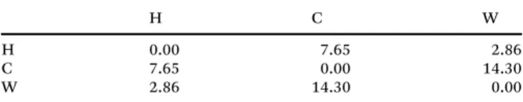
For instance, for the H3(C4)2/W (lipid/water) representation of ref. 44 considered here, with three particle types (KA{H, C, W}),
the mean field potentials are given by
VKðrÞ ¼kBT½wKHfHðrÞ þwKCfCðrÞ þwKWfWðrÞ
þkH½fHðrÞ þfCðrÞ þfWðrÞ f0
(9)
and the resulting forcesFKðrÞ ¼ rrVKðrÞon a particle of type
Kat positionr
FKðrÞ ¼ ðkBTwKHþkHÞrrfHðrÞ
ðkBTwKCþkHÞrrfCðrÞ
ðkBTwKWþkHÞrrfWðrÞ
(10)
The density fields fK(r) are defined on a uniform cubic
grid with spacingl. There is some flexibility of choice in the particle-to-field projection, and we assign particle fractions to neighbouring grid points using properly normalised Gaussians instead of the previous employed trilinear func-tions. This projection generates a less fluctuating field for the force calculation. Although these particle forces could be determinedviaa variational approach, we rely on the original grid-based method that calculates field gradients numerically using a staggered grid (see the appendix for more details) and we additionally consider another, more isotropic discrete gradient operator. In the remainder, we assume that the mass
mfor all particles is the same and set it to unity. Moreover, we also setkBT= 1.
Dynamics. As usual, new configurations are obtained by integrating the equations of motion from timettot+Dtby a velocity Verlet (VV) algorithm
riðtþDtÞ ¼riðtÞ þviðtÞDtþ12fiðtÞDt2 (11)
viðtþDtÞ ¼viðtÞ þ1
2ðfiðtÞ þfiðtþDtÞÞDt
for all particles in the system, where ri and vi represent the
position and velocity of the ith particle, and the force fi is
the sum of the intra-molecular forces and the mean field force, i.e. fi(r) = fintrai (r) + FK(r), withK the type of particle i.
For water particles, the absence of intra-molecular forces is reflected in fi(r) = FW(r), meaning that solvent particles only experience forces due to the density fields.
Although the MD-SCF model is essentially off-lattice, mole-cules only interactviasmoothed potentials that are defined on a (coarse) regular lattice. As a consequence, the contribution of particle collisions to the relaxation dynamics is largely underestimated, especially when the gradient terms practically vanish, for instance at large densities f0. In the original MD-SCF approach,26the VV-algorithm was combined with a (local) Andersen thermostat to mimic the effect of particle collisions and maintain a constant (kinetic) simulation temperature, by replacing the velocity of a number of randomly selected particles by a velocity drawn from a Maxwell distribution. However, such a local thermostat does not properly account for momentum transfer, as a result of a violation of Galilean invariance,30,32 and thus the relaxation dynamics is less realistic and generally very slow (see results section for examples). In principle, we could introduce Galilean invariance by another choice of the thermostat, see, for instance, the one developed in ref. 30, but this will not fundamentally resolve the discussed smoothing effect on collisions, and the computational penalty is consider-able, as such thermostats rely on computationally expensive pairwise velocity-difference calculations.
Multi-particle collision dynamics (MPCD)
The class of algorithms known as MPCD or stochastic rotation dynamics (SRD), a name that was used when the method was first formulated, combines discrete time with continuous space, and represents a fluid by point-like particles that undergo ballistic motion
ri(t+dt) =r(t) +vi(t)dt, (12)
withdta well-chosen time increment (streaming step). Particles only interact during collision steps, when momentum exchange takes place. Several energy and momentum conserving collision schemes have been proposed36 and share the property that, instead of pairwise velocity differences, only the center of mass velocity in each cell of a coarse grid needs to be calculated for a velocity update. It was shown that MPCD is Galilean invariant, provided that all cell positions are shifted by a well-chosen random vector prior to each collision step.35 Consequently, MPCD can be seen as a very simple and efficient numerical approach for solving the Navier–Stokes equations
and describing the hydrodynamics of viscous systems on a mesoscopic level.
Focussing on the collision step, the three-dimensional simula-tion volumeVis coarse-grained into cells of sizeaaa, witha
setting the resolution of the hydrodynamics. After shifting particle positions, by a random vectort= (tx,ty,tz)Twith components
tjA[a/2,a/2] (j=x,y,z) taken from a uniform distribution,35
particles are sorted to the cells and, for each cell, a center of mass velocity for thencparticles in the cell
vcm¼ 1
nc Xnc
j¼1
vj (13)
is calculated. The velocity update is given by
viðtþdtÞ ¼vcmðtÞ þ RðviðtÞ vcmðtÞÞ; (14) withvcmthe value for the cell in which particleiis located,dta time interval between collisions and R a 3 3 matrix that rotates vectors by a fixed angle a around an axis that is generated randomly for each cell.36After this update, particles are shifted back using the same random vector. The total number of particles, and thus the average number of particles per cellns, is a freedom of choice but remains constant during simulation. The algorithmic simplicity enables an analytic derivation of hydrodynamic properties in terms of parameters
ns,aanddt,via the Green–Kubo relations,37,38opening up a possibility of mapping to real systems.
Hybrid MPCD/MD.Despite its advantageous computational efficiency, standard MPCD does not apply to phase separating systems. In contrast to CGMD or DPD, where each particle represents a cluster of 3–4 solvent molecules with a base (excluded volume) repulsion in addition to non-ideal inter-actions, MPCD particles are point-like fictitious entities without potential-based interactions or relation to molecular detail. In other words, MPCD solvent can act as a momentum-conserving heat bath for any solute,39where solute particles can experience bonded interactions and should be included in the collision step, but the overall description remains that of an ideal and compressible gas. In particular, the lack of explicit interactions results in unphysical particle trajectories.
Fortunately, MPCD was recently extended to include the non-ideal interactions that play a role in many systems containing both solvent and solutes. One route, which was later formally linked to an equation of state for a system containing two particle types,40 is to introduce a new set of collision rules that acknowledges the different nature of colliding particles.41 The resulting algorithm was numerically tested by considering the phase behaviour of binary mixtures, analysing the spectra of capillary wave fluctuations on a droplet, and even by simulating phase separation in a ternary surfactant mixture.40Generalisation to many particle types, however, is not straightforward.
The second route is a hybrid MPCD/MD scheme developed and analysed by Malevanets and Kapral,42which couples a force-field based description for solute–solute and solute–solvent
interactions to an effective MPCD description for the solvent– solvent interactions. In short, the ballistic streaming step (12) is replaced by the VV scheme of MD, assuming that there are no solvent–solvent interactions besides collisions, and the two descriptions evolve on a different time scale. This hybrid MPCD/MD model serves as a basis in the present study.
Hybrid MD-SCF/MPCD scheme
An attractive solution for the very weak coupling between solvents and solutes in MD-SCF is to re-introduce particle collisions via
the off-grid multi-particle collision dynamics (MPCD) method, in which averaged particle velocities, calculated in lattice cells, are used to perform effective collisions between individual particles. By combining MPCD and MD-SCF, the implementation of which is discussed next, we restore the effect of particle colli-sions on the relaxation dynamics. At the same time, the method can be seen as a natural extension of the SRD/MPCD framework to complex and multicomponent fluids, reminiscent of the way Lattice Boltzmann (LB) was extended to complex fluids, by coupling it to a free energy functional.33,34
Our new hybrid scheme is very similar to the MPCD/MD scheme of Malevanets and Kapral,42but differs in the handling of the solvent, which is treated on the same footing as the solute during the streaming step. In the collision step, governed by the time intervaldtof MPCD, only solvent particles collide according to the update (14). In the streaming step, associated with a smaller time stepDt, both solute and solvent evolve according to the VV scheme (12). The force acting on each solute particle contains intramolecular (bond, angle, torsion) terms as well as non-bonded (intermolecular) contributions due to other solutes and due to solvent particles. In the MPCD/MD scheme of Malevanets and Kapral, the force acting on solvent particles stems only from the solutes, which is numerically efficient but can also be seen as artificial. In the new scheme, the forces on solvent particles are simply given byfi(r) =FW(r) of (10). Thus, besides the ‘standard’ contributions due to the solutes, albeit in terms of their density fields, there is another termkHrrfW(r) (note that a standard value forwWW= 0) that renders the force dependent on spatial variations of the solvent density field and stems from excluded volume interactions on the field level. This scheme reduces to MPCD/MD only forkH= 0. ForkHa0, any spatial variation of the total density fðrÞ ¼P
K
fKðrÞ from the reference valuef0will induce particle forces consistent with a reduction of this variation. Particularly in solvent-rich phases, fWEf0, this additional force term perturbs the solvent particle dynamics. By thus combining the MPCD/MD concept with the MD-SCF Hamiltonian, we obtain a more consistent description of the hydrodynamics of complex fluids, where one no longer has to distinguish between different components of the complex fluid. In the results section, we will quantify the effect of these additional force terms on the dynamics.
Momentum conserving thermostat.Momentum conservation is exact in standard MPCD, and the hybrid MPCD/MD scheme of Malevanets and Kapral42 conserves energy, meaning that a thermostat is superfluous when kinetic energy dominates, for
instance when solute particles interact only very weakly or when there is a strong mass misbalance between solute and solvent particles. For balanced systems, however, a thermostat may be essential for maintaining a constant temperature during simula-tion and, more in general, for the stability of the trajectory. This thermostat could be introduced at the MD level, for instance in the form of a Langevin-thermostat that couples to the relative velocity of the particles with respect to the mean velocity in their cell. Nevertheless, we select the Maxwell–Boltzmann scaling (MBS) thermostat,43which leaves the total momentum of a cell unchanged, since a thermostat on the MPCD level is most efficient. In this thermostat, the relative velocitiesDvi=vivcm of the particles in a collision cell are scaled by a constantxduring the collision step, withxa particular value for each collision cell. In MBS, the factor is defined as
x¼
ffiffiffiffiffiffiffiffiffiffiffiffiffiffi ^ Ek
Ek q
; (15)
whereEk¼1=2P nc
j¼1
mDvj2is the kinetic energy of thencparticles in a cell and Eˆk is selected from an appropriate distribution function for each collision cell.43In particular, the selectedG distribution converges to a Gaussian function with proper values for its mean and variance whenf= 3(nc1), the number of degrees of freedom of the fluid particles in the considered collision cell, goes to infinity. Solute particles are also thermo-statted during the collision stepviavi(t+dt) =vcm(t) +x(vi(t)vcm(t)). In particular, they are subjected to a velocity scaling that leaves the total momentum per cell unchanged, but not to rotation. After each thermostatting stage, any net momentum is removed by rescaling the mean particle velocity to zero.
On Galilean invariance.We should note that even though the underlying continuum Hamiltonian (7) is Galilean invariant, the sum over all forces (10) is not strictly zero due to discretization effects, hence momentum is not strictly preserved. Strict total momentum conservation can be imposed by adding an additional constraining force (a Lagrangian parameter) in each step. We have tested this and found that this may affect the results if we use the gradient operator introduced by Milano and Kawakatsu,26but not if we use a more isotropic gradient operator introduced in this paper. Furthermore, we found that discretization effects could be reduced significantly if the inertial frame of the simulation was chosen such that the discretization grid moves with a constant background speed. Details are discussed in Appendix C.
Practical implementation of MD-SCF/MPCD for a lipid model
It is good to realise that one may select any coarse-grained molecular representation in the hybrid approach. Whereas the original MD-SCF approach benefits from selecting a familiar Martini representation for which many biomolecules/solvents have been parameterised, it introduces the necessity to deter-mine a map between the Martini force fields and effective FH-parameters.26For the purpose of illustration, we instead select the DPD representation of Shillcock and Lipowsky,44i.e.lipids are represented by a H3(C4)2chain (Nl= 11 particles), for which
a mapping to FH-parameters already exists. Like in CGMD, 3–4 water molecules constitute one W particle. In particular, since the hybrid method represents all intermolecular interactions at a field level, the treatment of the solvent phase (as single particles) is equivalent in both representations.
We distinguish dimensionless variables from physical quan-tities by an asterix. As usual in DPD,44we scale length and time asr* =r/rcandt¼t
ffiffiffiffiffiffiffiffiffiffiffiffiffiffiffiffiffiffiffiffi kBT=mrc2 p
, withrcthe cutoff distance of DPD. This scaling corresponds to the choicem= 1,rc= 1 and kBT= 1 of reference units. Important SRD/MPCD variables are the cell sizeaMPCD=rc(aMPCD* = 1), unless specified otherwise, and mean free pathl¼dt ffiffiffiffiffiffiffiffiffiffiffiffiffiffiffiffiffiffiffiffiffiffiffiffiffiffiffiffiffiffikBT=maMPCD2
p
(l* =dt* foraMPCD* = 1). Initially, all N particles are placed in a cuboidal system of constant volume V = LxLyLz (all sizes in units of rc), so that the overall particle density f0* = N/V* (V* = V/rc3) is fixed. The first lipid head (H) particle and all solvent particles are usually placed at random. In setting up a simulation, choices for the densityf0* and sizeV* provideN =f0*V*, whereas a choice for the number of lipid chainsnldefines the number of water particles asnw =N Nlnl. All simulations start from a Maxwell–Boltzmann distribution for the particle velocities at a given (kinetic) temperatureT, with an average kinetic energy
mhv2i = 3kBT. The configurational temperature is sometimes advocated as a better measure,45but it is based on the gradient and Laplacians of the interaction potentials, so we rely on the standard procedure of monitoring the kinetic tempera-ture h(v*)2i/3 instead. In all simulations, periodic boundary conditions are used. Although all simulations for lipid/water systems were repeated with 3 different noise seeds to check consistency, all reported results are for individual simulation trajectories.
The strength of the ‘soft’ (quadratic) DPD interaction poten-tials is given by the expressionaij* =aii* +Daij* (usinga* =arc/kBT), withaii* = 75/r0*.21 For the usual density ofr0* = 3 (aii* = 25),
Groot and Warren developed a mapping between the mean-field FH parameters (w4 2) and Da* for mixtures of single particles as21
w= (0.2860.002)Da* (16) or, for short chains,
w= (0.3060.003)Da*. (17) Using expression (16) for the water–lipid and (17) for the lipid– lipid interaction to convert theDa* for the chosen DPD parameters,
i.e.DaKK* = 0 for KA{H, C, W},DaHC* = 25,DaHW* = 10 and
DaCW* = 50,44we obtain the values shown in Table 1. Matching the equation of state for the pressure, a value for the
Table 1 The dimensionless interactionwKK0for particles of type K
inter-acting with a density field due to particle of type K0. Mean-field interactions between the same particle types are zero by definition
H C W
H 0.00 7.65 2.86
C 7.65 0.00 14.30
W 2.86 14.30 0.00
dimensionlesskH* was previously obtained askH* =kHnp/kBT= 5.0 (withnpthe particle volume) for the same particle density.14 The FH parameters of Table 1 have been used in all simula-tions for the lipid–water system discussed in the results section. However, these parameters relate to the usual situation where the average of the total field is conveniently scaled to unity (via
multiplication by an appropriate particle volume). In the projec-tion algorithm, density fields are obtained from a particle-wise assignment of particle fractions to neighbouring grid points (summing up to one), followed by an additional point-wise multi-plication of the density fields by a factor 1/(l*)3, which has the purpose of rendering the average total fieldf* independent of the grid sizel. In particular, definingnx=Lx/l,ny=Ly/landnz=Lz/l,
and writingr= (i,j,k) in units of the mesh sizel, it is easy to show
f¼ 1 nxnynz
X
K X nx;ny;nz
i;j;k¼0
fKði;j;kÞ
l
ð Þ3
¼ N
ln
x ð Þ ln
y
ln
z ð Þ
¼ N
LxLyLz ¼ N
V¼f0
(18)
Since we are working with this non-unitary total field, we have to scalewKK0by 1/f0*.
MD-SCF/MPCD is based on the Hamiltonian (7) and evolved using MD (velocity Verlet) and MPCD, which both conserve energy, so we simply conclude that our method is energy conserving. Focussing on numerical stability, the ‘safe’ upper bound for Martini CGMD,i.e.Dt= 30 fs,28was consistently used for all MD-SCF simulations (with an Andersen thermostat) that employed a Martini representation for their constituents.26 When applying MD-SCF/MPCD instead, this value seems a conservative but safe choice. However, since bonded interac-tions are not affected by the hybridisation, a DPD-like time step can be expected for the current lipid/water representation, which is adopted from DPD. As discussed by Groot and Warren,21 the choice of the dimensionless time step Dt* in DPD is determined by the amount of increased/artificial tem-peraturekBT*1 that one is willing to accept: they define the safeDt* as the one for which this increase is 2%. For brevity, we refrain from showing all temperature evolutions in the Results section, but we only note here that our choice forDt* = 0.01 was based on a quick levelling of the simulation temperature to a constant value that is consistently about 2% higher for this time step, for all lipid/water MD-SCF/MPCD simulations con-sidered. We thus conclude thatDtE3 ps, which is estimated
viathe properties of water particles, is a safe choice: it is indeed in the same range as the earlier reported DPD value of 5 ps for this lipid model.44 However, as field projection is usually not performed every time step in MD-SCF/MPCD, e.g. for the solvent (lipid/solvent) systems, it is performed every tenth (fifth) VV step respectively, see discussion at the end of this section, selecting even largerDt* may result in instability. We indeed find thatDt* = 0.02, the value employed for all DPD simulations in this study, results in a fluctuating,
non-monotonic evolution of the simulation temperature when used in MD-SCF/MPCD for the lipid/solvent systems. However, when the field is projected every time step instead (fup = 1), we recover proper behaviour withkBT* 1 o2%. Sincedt*/Dt* is necessarily an integer, we also tried Dt* = 0.05 (stable,
kBT*1E2%) andDt* =dt= 0.1 (unstable), quantifying the direct relation between the maximum safe time step and the field projection frequency. Also in the MD-SCF/MPCD simula-tions for pure solvents, where the field is updated every tenth time step forDt* = 0.01, the temperature increase is less than 2% for all values ofkHconsidered.
Finally, we have to select a proper grid sizel=l*rcfor the projection of particles to density fields (see the appendix for more details). Among other, this defines the resolution of the fields and forces in the hybrid model, which should be chosen wisely given the application in mind. First, we note that we are limited in the range ofl-values at the lower end if we stick to the standard choice for the particle density f0* = 3 of DPD. The average number of particles per MPCD cell should be in the range 3–20,46 so this is a proper choice also for MPCD. However, since the projection algorithm only considers neigh-bouring grid points, field gradients and thus the effective forces on the particles will become increasingly noisy for smallerl*. Forl*o1 andf0* = 3, for instance, there will be less than three particles per grid cell on average, and it is easy to understand that very minute particle displacements will have a tremendous effect on the field gradients. As a compromise between resolution and smoothness, we choosel=rcorl* = 1, meaning that 5 grid points should suffice to describe the lipid profile (as well as field gradients for the force calculation) for a lipid membrane, which has a thickness of roughly 5 nm. Moreover, we use a Gaussian, evaluated on 27 points around the closest grid point to the particle, rather than the original trilinear interpolation on 8 points, for the reasons discussed before. From these considera-tions, it is clear that we do not expect to reproduce the membrane profile of DPD in full detail. However, we note that a CGMD lipid representation is better resolved in space, enabling a smaller choice of l*. Moreover, smaller values of l* are possible for our DPD lipid representation, either by selecting a projection algorithm with additional grid points, which has the effect of further smoothing, or by choosing a larger particle densityr0* (or, equivalent, a smallerrc). As the particle-to-field projection is the most compute intensive procedure, both will be at the expense of a reduced computational efficiency.
The frequency with which the projection algorithm is called,
fup, is an important parameter for the computational efficiency; an update frequency offup= 10,i.e.in which the projection algorithm is called every tenth time step, was considered in the original MD-SCF model, and even larger values were found suited in specific cases.29This value is determined by the optimum between efficiency and both the effective particle dynamics and field resolution, in particular how fast the density fields at the chosen resolution changes given the underlying particle dynamics. The valuefup= 10 was considered a conservative choice,29and we will use it as the initial value. Nevertheless, later on, we discuss the need for using smaller values.
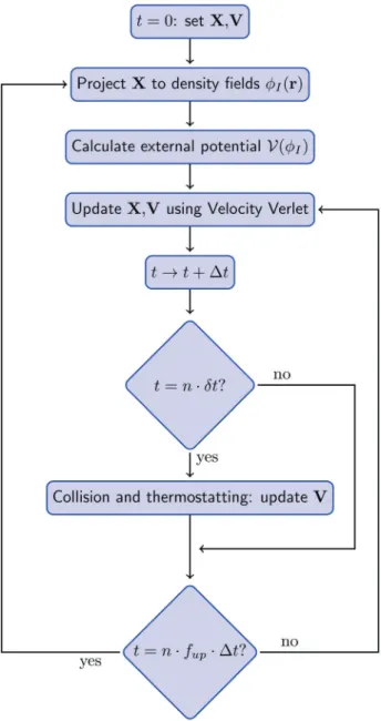
Flow diagram for the current method, withXandVdenoting the position and velocities of all particles, n an (arbitrary) integer, dt the time step for collision and fup the update frequency for the field projection.
Computational analysis
When evaluating the performance of new methodology, one should be careful in separating the various aspects that contribute to efficiency. The first is the implementation into a computer algorithm, which enables a useful quantitative evaluation of efficiency in terms of the number of floating point operations (or the CPU time that they require) per time step in comparison to reference methods. The second are the conceptual steps made to generate a more efficient description of the underlying physics, herevia(partial) coarsening and by accounting for the long-range hydrodynamic interactions.
The algorithmic advantage of hybrid MD-SCF/MPCD over pure-particle reference methods like (CG)MD and DPD, is the
replacement of the force calculation for particle pairs by one that stems from particles interacting with chemical potential fields, after particle-to-field projection, which reduces the costs of this step and enables more efficient parallelisation.27 Nevertheless, the key advantage is the alternative physical descrip-tion: since we replace the ‘hard’ Lennard-Jones interactions in (CG)MD by ‘soft’ mean-field interactions in MD-SCF/MPCD, we may replace the usual time stepDtBfs that is required for stable integration in (CG)MD by theDtBps time step of methods that consider soft-core interactions, like DPD. As a consequence, the sampling in the time domain is enhanced by several orders of magnitudes, unless bonded interactions dictate otherwise or the reference methods is already based on soft-core potentials. Since MD-SCF/MPCD inherits this property from MD-SCF, we refer to the literature for a detailed analysis.29 Furthermore, coupling MD-SCF to MPCD substantially accelerates the self- and re-organisation kinetics, see Results and discussion section, by restoring the hydrodynamic contribution to such processes.
We simulated a lipid/water system in two different volumes,
V1 = 223l3 and V2 = 443l3, containing N1 = 31 944 particles (764 lipids) andN2= 255 552 particles (3058 lipids), respectively. The number of lipids agrees with a flat membrane that spans the volume along two Cartesian coordinates. Table 2 shows timing results for algorithms that only differ in the implementation of the force update, the thermostat and/or the collision step. The depicted timings for a single time stepts(V) (in CPU seconds) were obtained by averaging over a total of 104time steps for each simulation. We find that MD-SCF/MPCD is roughly a factor of two faster than DPD: 1.7 forV1and 2.3 forV2. SinceN2= 8N1, perfect scaling relates to a scaling factorz=ts(V2)/ts(V1) = 8, if we disregard the costs of the intramolecular forces calculation. Apparently, updating neighbour lists is demanding, as we find z= 10.86 for DPD, whilez= 8.00 for both other methods. The costs of the MPCD collision step are modest (E1% of the total). A comparison of MD-SCF/MPCD for fup= 5 or 10 shows that considerable computational gain can be obtained by performing fewer updates of the projection algorithm.
Results and discussion
Pure solvent systems
The hydrodynamic properties of a fluid simulated by MPCD/ SRD were considered in detail.47 This study identified two
Table 2 Time (averaged over 104time steps) in CPU seconds required for performing one (time) step with each of the three considered methods/ algorithms. Results were obtained using very similar serial codes, on a 2.8 GHz Intel Core i5 node with (shared) 8 GB 1333 MHz DDR3 memory
VolumeV(inl3) ts(V) (in s)
DPD 223 0.2261
DPD 443 2.4561
MD-SCF, Andersen 223 0.1311
MD-SCF, Andersen 443 1.0473
MD-SCF/MPCD,fup= 5 223 0.1321
MD-SCF/MPCD,fup= 5 443 1.0530
MD-SCF/MPCD,fup= 10 443 0.7206
regimes, a gas-like and fluid-like, quantified by the Schmidt number Sc = n/D, i.e. the ratio between viscous (kinematic viscosity n) and diffusive (diffusion coefficient D) transport coefficients. Moreover, it was found that the combined value ofl*, the scaled mean free path, anda, the rotation angle in the collision step, regulates this character. By considering the predicted Schmidt number Scp,i.e.using thenandDestimated from simulations, a fluid-like collective regime with Scpc 1 was identified for largeaand smalll*, and for smallaand large l* a gas-like particle regime with Scpr 1. The microscopic motions underlying the dynamical behaviour of the fluid were analysed via the normalised discrete velocity autocorrelation function (VACF) forl* = 0.1 (collective regime) and 1.0 (particle regime),i.e.
CvðtÞ ¼
viðtÞ við0Þ
h i
við0Þ við0Þ
h i; (19)
wheret=ndt* is the discrete time relative to the starting time
n0dt* at the origin, andhidenotes an ensemble average over all particles andn0.
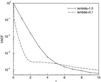
To test our implementation, we calculated the VACFs for bothl* for the same parameter set (with angle of rotation a= 1301) of the earlier study,47 see Fig. 1. Since this system is
ideal and the collision rules (14) conserve momentum and kinetic energy exactly for a fixed angle of rotationa, a thermostat is not needed. All VACFs in this section were obtained by simple averaging over the last 4.9104consecutive time steps and over 10 independent simulations, each of which is started with a different noise seed. We note that especially the long time VACF behaviour is sensitive to the sampling statistics. From a comparison of Fig. 1 to Fig. 3 in ref. 47, we find that we reproduce the older results in this time regime.
Another important test is to analyse self-diffusion. Diffusion coefficients can be derived from the Green–Kubo formalism, but Ripoll et almention that a linear fit of the mean-square displacement (MSD) for long times provides equivalent results.47 Fitting the MSD for our simulated systems, we find
D* = 0.64 forl* = 1.0 andD* = 0.080 forl* = 0.1. Explicit values were not reported before, but we may compare the relative deviationDD= (DsimD0)/D0, withD0an analytical prediction obtained using the Brownian approximation for the VACF in the Green–Kubo relation.47We findDD= 0 forl* = 1.0 andDD= 0.25 forl* = 0.1, which is fully consistent with known results for the same parameter set, shown in Fig. 7 of the earlier study.47
Turning back to the VACF, forl* = 1.0 and short times it closely follows the exponential decay that was predicted for a dense gas, in agreement with the system being in the particle regime. For l* = 0.1, however, the behaviour of the VACF at shorter times deviates considerably from a gas-like exponential decay, signalling that cooperative effects play a role in slowing down the loss of velocity correlations over time. However, the VACF does not exhibit the typical negative region associated with backscattering or collective relaxation,i.e.transient caging imposed by neighbouring particles. At longer times, both VACFs decay algebraically as t3/2,47 in agreement with the
theoretical universal scaling relation for fluids in thermal equilibrium,48see Fig. 2.
Backscattering or a negative region in the VACF is also absent for DPD simulations with only excluded volume interactions,45 whereas it was already observed in MD simulations of liquid water by Rahman and Stillinger,49 where non-bonded inter-actions are represented by Lennard-Jones potentials. The distinct oscillatory behaviour of the VACF of liquid water around the origin in the latter study, compared to simpler liquids that only carry one negative minimum, was attributed to hydrogen bonding, which results in a greater structural rigidity.49 We note that the particulars of the monotonic VACFs in DPD depend on numerical parameters, e.g. the chosen time step, and can be tuned by the choice of the friction coefficientg. For the usual DPD valueg= 4.5, the VACF is visually very similar to the one obtained for MPCD andl* = 0.1.45
The effect of caging on the short-time transport properties is clearly not captured by the coarse treatments like MPCD and DPD, which lack the interactions that are responsible for this effect. One could, however, wonder what role compressibility plays in this phenomenon. Although the standard MPCD/SRD method does not impose incompressibility in any way, by design, the deviations of the solvent field fW*(r) (obtained using the projection algorithm) from the reference value f0* are limited at all times in practice. We may, using the same notation as before, monitor the time-dependent varianceO(t) of the solvent field,i.e.
OðtÞ ¼ X nx;ny;nz
i;j;k¼0
fWði;j;k;tÞ f0
ð Þ2 (20)
Fig. 1 The normalised VACFversusdimensionless timet* (half log plot) for two values of the scaled mean free path:l* = 0.1 (collective regime, dashed line) andl* = 1.0 (particle regime, solid line). For bothl*, all other parameters are the same. In particular, we selected the same MPCD and volume parameters as in Fig. 3 in ref. 47 to test our implementation: cell sizeaMPCD* = 1.0, densityr0* = 5,a= 1301andLx* =Ly* =Lz* = 20. This
choice for the cell size implies thatdt* =l*. The shown graphs were obtained by averaging over the last 4.9104consecutive time steps and over 10 independent simulations, each of which is started with a different noise seed.
to analyse the compressibility. Since MPCD solvent behaves as an ideal gas, the discrete probability P(nc) for finding nc particles per lattice cell is theoretically given by a Poisson distribution
P nð Þ ¼c nc h inceh inc
nc!
; (21)
withncthe number of particles per cell andhnci=ns=f0* their average value. As a consequence of the variance per lattice cell beingf0* in the steady state, we find thatO(t) =Ost=V*f0*.
Analysing O(t) from the simulations for V* = 4000 and f0* = 5, the first observation is that O(t) quickly reaches a plateau valueOthat does not depend onl*, consistent with it being an equilibrium property. However,Ois lower than the theoretical valueOst= 40 000, namelyO= 2606 with standard deviationsO= 99 forl* = 1 andO= 2607 andsO= 103 forl* = 0.1.
This deviation can be understood in terms of smoothing due to the particle-to-field projection, which assigns particle fractions instead of particles to lattice positions. As a result, the number of particles per cellsNpis usually a fractional number and thus the probabilityP(Np) is a continuous instead of a discrete function. In particular, if we enforce discrete particle assignment, by projecting each particle fully to the closest lattice position, both the Poisson distribution and the theoretical valueO=V*f0* are recovered. From simulations with the original trilinear and the new Gaussian projection schemes, for different values off0* and
V*, we find the relation O =sV*f0*, containing an additional constantswhich is fitted as 0.295 (E3/10) for trilinear and 0.064 (E1/15) for Gaussian interpolation. We note that the particle evolutions, and thus the equations of state, do not depend on this projection: they are the same in all considered cases. It just show that the variance of the projected solvent field depends on the projection algorithm. As expected, the smoothing is most significant for the Gaussian projection algorithm.
These numerically obtained values for an ideal gas can be used for a comparison to the new hybrid MD-SCF/MPCD method, which includes a field-based compressibility term. For the sameaandl* = 0.1, we replace the ballistic motion of MPCD by the velocity Verlet (VV) scheme (12) with a non-ideal force
fi(r) = kHrrfW(r) for all particles and a time step Dt. The collision step, carrying a time stepdt, is the same as in (14). Note that we recover the original MPCD scheme when the compressibility term is omitted (kH= 0). Due to the excluded volume interactions, the kinetic energy is not necessarily con-served, and we apply the MBS thermostat during the collision step to maintain a constant simulation temperature. The time increment for the VV-scheme isDt* = 0.01. Forr0* = 5, a value of kH* = 3 was determined earlier,14which sets a realistic range for the Helfand parameter. The fieldfWis updated withfup= 10, i.e.at every collision step.
Fig. 3 shows the short-time VACF for these systems for different values of the Helfand compressibility parameter kH in this range. We find that adding excluded volume interac-tions gives rise to effective caging, as can be concluded from the presence of negative regions in the VACF. The origin of this phenomenon lies in the understanding that particles experi-ence a force that drives them towards a situation where the variance of fW(r), the field derived from the instantaneous particle positions, decreases in between collision steps,i.e.large fluctuation of the solvent field are suppressed. In particular,
O(kH*) decreases for increasingkH*, see Fig. 4, as one may expect, indicating also that sound waves are not an issue. Since these forces oppose the build-up of regions of too low and high
Fig. 2 Log–log plot of the same data as in Fig. 3, forl* = 0.1 (triangles) and l* = 1.0 (circles), including the long-time tails. A: full time range, and B: zoom of tails. Lines relate to the predicted algebraicBt3/2decay of the VACF, with an amplitudea0that is either obtained from the best fit to data points in a selected range (t* A[6,20], solid line) or explicitly derived from mode-coupling theory asa0= ((d1)/dr)(4p(D+n))d/2(dashed-dot line), see also Fig. 4 and discussion in ref. 47. To evaluate the latter expression, diffusion coefficients D extracted from simulations were used and the kinematic viscositynwas estimated from Fig. 1 and 2 in ref. 47 and the relation Sc =n/D, giving rise ton* = 0.80 forD* = 0.080 (l* = 0.1, ScE10) andn* = 0.64 forD* = 0.64 (l* = 1.0, ScE1), insertingd= 3 andr* =r0* = 5. Like in the previous study,47we find that the predicted amplitude is exact within error bounds forl* = 1.0 and that it is about 10% larger than the fitted one forl* = 0.1. Nevertheless, the zoom shows that the predicted decay (dashed-dot line) is reproduced forl* = 0.1 at late times,i.e.next to the time range (t*Z20) where finite size effects start to dominate.47Since we are interested in analysing how compressibility modulates the VACF, we will use both functions as a reference in the remainder.
particle densities, particles experience an effective caging by their surroundings.
Our treatment deviates in this aspect from the original hybrid approach of Malevanets and Kapral,42 which neglects all solvent–solvent interactions in the MD propagation scheme between collision steps. Their theoretical analysis of MD/SRD as a numerical solver for the Navier–Stokes equations starts
from the ballistic streaming step for solvent particles, and it is not directly apparent if and how including direct solvent– solvent interactions in the MD updates, like the ones advocated here, affect this hydrodynamic description. Padding and Louis50 did introduce additional terms in the inner MD loop for a pure solvent system, but they restrict themselves to external forces (due to gravity, fixed or moving boundary conditions) on solvent particles and disregard any direct force between solvent particle pairs. Disregarding them, however, seems to be purely a matter of convenience and not a methodological constraint.50After all, representing solvent–solvent interaction only by collisions is favoured in terms of computational efficiency and analytical tractability.
Instead of a formal justification, we may study the longer-time scaling for the simulated systems withkH*40. In Fig. 5, we have plotted the absolute value of VACF versus t* for the three considered values ofkH* on a log–log scale. The algebraic fitting functions shown in Fig. 2,i.e. a0t3/2witha0determined either by regression or from mode-coupling theory, both for l* = 0.1, are added to enable a direct comparison to the results of the original MPCD scheme. We note that, as before, the behaviour starting from t* E 15–20 can be attributed to the finite system size and should be disregarded in this analysis.47 Although the trends are certainly less well-defined than for kH* = 0, the known algebraict3/2decay is reproduced reason-ably well by the simulations results forkH*a0, most clearly for kH* = 1 and 2. This analysis suggests that the hydrodynamics on a larger scale is not significantly affected by the introduction of the (weak) particle pair interactions, but a formal derivation is left for the future. Also intuitively one could expect this finding, since the original collision scheme is conserved. The diffusion coefficient, obtained from the MSD for these simulations,
Fig. 3 The normalised VACF versus dimensionless time for a non-cohesively interacting gas (w= 0) in the new MD-SCF/MPCD approach, where compressibility is penalisedviathe Helfand compressibility term in the non-ideal free energy. ForkH* = 0, standard MPCD is recovered. The graphs show results for increasing compressibility parameter:kH* = 1 (black, circles),kH* = 2 (red, squares) andkH* = 3 (blue, diamonds). The latter value relates the compressibility of the system to that of liquid water at room temperature. We used the same system parameters as before and a MPCD time stepdt* =l* = 0.1 (collective regime). The time step for the VV scheme (12) isDt* = 0.01. The shown graphs were obtained by averaging over the last 4.9104consecutive time steps and over 10 independent simulations, each of which is started with a different noise seed.
Fig. 4 The mean valueOof O(t) in (20) for different values ofkH*, as determined over the whole trajectory. In the simulations,O(t) very quickly levels off to a constant value around which it fluctuates. Bars reflect the standard deviationsOof these fluctuations. From the observation thatO
monotonically decreases for increasing kH*, we conclude that sound waves play no role when compressibility is accounted for. In particular, unphysical sound waves are absent forkH* = 0 (standard MPCD).
Fig. 5 Log–log plot of the absolute value of the normalised VACF shown in Fig. 3, forkH* = 1 (black, circles),kH* = 2 (red, squares) and the realistic value kH* = 3 (blue, diamonds), zooming in on the long time tails behaviour. Taking the absolute value is required because of the negative regions in the VACF. The algebraic decaya0t3/2of standard MPCD is added for comparison, see Fig. 2. Solid line: with numerically fitteda0; dashed-dotted line: fora0calculated using mode-coupling theory.
isD* = 0.079 for allkH*a0 (compare toD* = 0.080 for standard MPCD withkH* = 0). This finding confirms that self-diffusion is hardly affected by the additional control of the compressibility. In addition tofup= 10, where the field is projected every tenth VV step or every collision step, we have performed simulations forkH* = 3 and field updates every fifth VV step,i.e. fup= 5, the standard value in the next sections, and even every VV step,
i.e. fup= 1 (fully synchronised). The original model of Milano and Kawakatsu generally employed much fewer updates, i.e. fupB 10–100,29based on the observation that projected fields are usually only slowly fluctuating. Although fewer updates are certainly computationally attractive, it also signals that the underlying particle dynamics in the MD-SCF model is rather slow. Selectingfup= 1 can be seen as a test for the consistency between the field projection and the underlying particle dynamics in the current treatment.
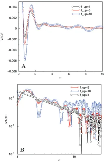
Fig. 6 compares the short time and long-time behaviour of the VACFs forfup= 10,fup= 5 andfup= 1. Again, we may disregard the very long-time tails, where the restricted system size becomes an issue. It is clear that also the VACF for the fully synchronised case contains a negative region and that the graph oscillates, albeit that the amplitude of these oscillations is significantly smaller than for fup = 10. The latter can be understood in terms of the temporarily static nature of the concentration field forfup41. Since the particle dynamics is driven by this field, updating the field less frequently (fup= 10) is equivalent to increasing the equilibration time towards an optimal particle configuration given that (static) field, which clearly enhances the caging. The position of the local VACF minima, however, does not notably depend onfup, and filtering these VACFs, to damp the oscillations, shows that they feature equivalent long-time behaviour. The algebraic long-time decay (Bt3/2) is already quite apparent forfup= 1.
Lipid–solvent systems
Next, we consider systems containingnlH3(C4)2lipids andnw single-bead W solvent in a volumeV* =Lx*Ly*Lz* of varying size,
subject to periodic boundary conditions. The grid size l for the particle-to-field projection is usually set tol=rc(l* = 1), but we will also consider other values. As mentioned before, we renormalise the overall particle density, which varies withl, to f0* after every particle-to-field projection. Here, we consider the standard value f0* = 3 for DPD. The total number of particlesN is constant and given asN=nw+ 11nl= 3V*. The FH parameters are fixed in all simulations,i.e. wHC = 7.65/3, wHW = 2.86/3 and wCW = 14.30/3 (see the Simulation setup subsection). The average area per lipid A for a tensionless membrane was previously determined as A0¼1:26 (in units ofrc2).44We determined an equivalence between the compres-sibility parameterkH = 5 and the DPD aii= 25 for a particle
density f0* = 3, via the equation of state for the pressure, although we used kH = 4.6 before.14 Since this parameter controls the lipid spacing within a membrane, we will vary its value within this small range.
To test whether our set of thermodynamic parameters {wKK0,kH} provide a proper mapping between the hybrid MD-SCF/MPCD
and the reference DPD model, we initially distribute a well-chosen number of lipids,i.e.nl¼2LxLy=A0, at random locations in the volume. By selecting nl consistent with a flat or planar tensionless DPD bilayer along two Cartesian directions, the sensi-tivity of the surface tension to the average area per lipidA44in our NVT ensemble is exploited. Spontaneous self-assembly in the hybrid model should give rise to a planar bilayer; if another (tensionless) structure is formed, either it is a metastable state or our parameters should be tuned. For reasons of efficiency, we avoid a field update at every time step, but instead select a small value fup= 5, assuming that the field does not signifi-cantly change between updates for this value. It was deter-mined from test simulations for differentfupand it is actually Fig. 6 Comparison of the normalised VACF forfup= 10 (blue, diamonds), fup= 5 (red, squares) andfup= 1 (black, circles) forkH* = 3. The time step for the VV scheme (12) isDt* = 0.01 andl* =dt* = 0.1 in the MPCD part. All other parameters are the same as in Fig. 3. A: the normalised velocity autocorrelation functionversusdimensionless time. B: log–log plot of the long-time tails of the absolute value of the normalised velocity auto-correlation functionversusdimensionless time. The algebraic decaya0t3/2 of standard MPCD is added for comparison, see Fig. 2. Solid line: with numerically fitteda0; dashed-dotted line: fora0calculated using mode-coupling theory. The shown graphs were obtained by averaging over the last 4.9104consecutive time steps and over 10 independent simulations, each of which is started with a different noise seed.
smaller than the usual minimal choice in MD-SCF,29 in line with our expectation that the field evolution is accelerated by accounting for collisions. The cell sizeain the MPCD scheme is initially chosen as small as possible,a* =l* = 1, to maximise the resolution of MPCD. We note that this choice relates to roughly 3 particles per collision cell, which is fairly small compared to the usual values of 5–15,47 but within the range where MPCD is valid.46The rotation angleaand collision time stepdtin MPCD are set toa= 901anddt* = 0.1, which positions the dynamics
in the solvent domain in the fluid-like regime.47 The time step used in the VV-scheme is Dt* = 0.01, with collisions (and thermostatting) thus taking place every 10 steps of the inner loop.
Consistency of the MD-SCF/MPCD parameters. We start with a small cubic volumeV* (Lx,y,z* = 22) containingnl= 764 lipids and nw = 23 540 solvent particles. The reference DPD simulation, using parameters of Shillcocket al.,44shows that a planar membrane readily forms by breakup and coarsening of an initially interconnected structure. Close examination of the structural evolution, however, shows that the limiting factor is the diffusion and uptake of solvated lipid micelles (here: one micelle) that result from this breakup process. After approxi-mately 105time steps, withDt* = 0.02, this process is completed (see Fig. 7A and A0).
Next, we consider the same system using our new hybrid model, varying the compressibility parameter betweenkH= 4.6 (ref. 14) andkH= 5.0, the theoretically predicted value for this
density. When both the changes in the non-ideal free energy
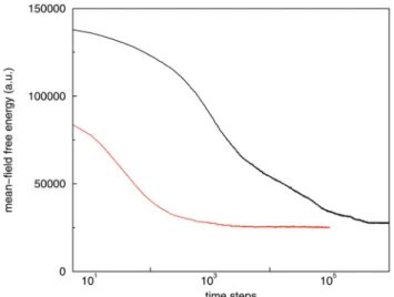
W[f] and the lipid structure are negligible beyond a certain stage, we denote that structures as equilibrium. ForkH= 4.6, lipids rapidly assemble from a mixed phase,viaintermediate spherical and cylindrical micellar phases, into a stable space-filling interconnected structure on a large scale, see Fig. 7B, while a planar lipid bilayer, aligned with two of the Cartesian axes, rapidly assembles forkH= 5.0 (Fig. 7C). Considering the structure for kH = 4.6, which is exemplary for a (meta)stable structures in the rangekHA{4.7,4.8,4.9}, more carefully, we find
that the lipid–water interface is reminiscent of a unit cell of a Schwarz minimal surface type P,i.e.a triply periodic surface with minimal surface area and vanishing mean curvature, albeit that it is slightly distorted. We note that continuing this simulation, up to a total of 2105time steps confirms that the structure shown in Fig. 7B is (meta)stable.
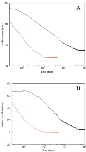
To obtain a better insight in the peculiarities of the simulation results, we quantify all structures in terms of geometrical and topological features of the lipid–water interfaceviaa procedure that determines the four Minkowski functionals (MFs) for the total lipid field,fl(r) =fH(r) +fC(r).51,53For the interconnected equilibrium structure shown in Fig. 7B, one of the MFs, the Euler characteristicwMF, is indeed2, which is the theoretical value for the unit cell of a P-surface.52,54Other theoretical MF values for a P-surface unit cell are 0.5 (volume), 2.345 (surface area), and 0 (integral mean curvature).54 For the planar membrane, we find wMF= 0 as a result of the periodic boundary conditions, which relate this structure to a vesicle, i.e. a spherical object with one internal cavity.51Before analysing the geometrical MFs, we note that our procedure overestimates actual values for curved surfaces because of the two-fold discretisation, from particles-to-field and field-to-voxels, that is needed for our procedure,54 unlike the topological Euler characteristic, which has an integer value that is not affected by the discretisation procedure. We nevertheless consider our procedure sufficient for the current analysis. For more sensitive analysis,e.g.to properly analyse the geometrical properties of the bicontinuous connection region that forms upon fusion between two membranes, the calcula-tion procedure could in principle be improved by using a finer grid to project particles directly to voxels instead of using field values on the fixed computational grid.
Comparison of the MFs that are related to the total surface area and integral mean curvature, along the pathway for the two values of kH, shows that the characteristics of structure evolution overlap in the initial stages, see Fig. 8. Moreover, the decrease of the integral mean curvature to zero with time forkH= 5 confirms the completion of a planar bilayer around 104time steps.
We may alternatively view our membrane as a thin elastic sheet, and write a Helfrich effective surface HamiltonianHfor a symmetric bilayer membrane
H ¼ ð
A
dS sþ2kcH2þkK
; (22)
withsthe surface tension,Athe total surface area,kcandkthe bending modulus and Gaussian bending modulus, respectively,
Fig. 7 Simulation snapshots after 20 000 (A) and 100 000 (A0) time steps of DPD (Dt* = 0.02). Just prior to the stage shown in the right hand side, a long-lived lipid micelle has merged with the bilayer. (B) Simulation snapshot after 10 000 steps of the new hybrid method forkH = 4.6. (C) Simulation snapshot after 10 000 steps of the new hybrid method for kH= 5.0. The mean-field free energy for the structures in the bottom row, obtained usingDt* = 0.01, has reached a constant value, suggesting that they are equilibrium structures. For clarity, only H3(C4)2lipids are shown, with red/blue representing H/C particles. In all simulations, periodic boundary conditions were employed.
andH= (c1+c2)/2 andK=c1c2the local mean and Gaussian curvature, with c1 and c2 the local principal curvatures. Although a thin elastic sheet representation is not adequate for small lipid domains with high curvature, i.e. some of the simulated structures in this study, it is not uncommon to seek additional insight by employing Helfrich theory also for these cases. For the membrane considered here, the bending modulus was previously determined as kc = 25kBT and the number of lipids consistent with a tensionless flat membrane,60 although one could wonder if these values are also appropriate for MD-SCF/MPCD. The termkKin (22) is usually omitted, as it is constant when the Euler characteristic does not change,via
the Gauss–Bonnet theorem. Moreover, it vanishes for a structure withK= 0, like a planar or cylindrical structure, if we neglect shape fluctuations that are unimportant for our analysis. The challenge here is that the Euler characteristic for a plane and
a P-surface are different, and the Gaussian curvature for the P-surface is non-zero, meaning that the extra term should be added to compare the Helfrich energy for these two structures. A planar membrane (H= 0) that is tensionless (s* = 0) for an average area per lipidA4A0, as a result of an unmatched kH, will experience a non-zero (positive) surface tensionswhen assembled from a number of lipids consistent with A0.44 A mismatch ofkHwill therefore destabilise a planar membrane in favour of structure associated with lower surface tension, as long as the topology does not change. The number of accessible structures or states, however, is limited by the forced periodicity in all three dimensions, which rules out simple tilting to relieve surface tension, and will thus affect the barriers between accessible states. The quadratic term in (22) vanishes for a triply-periodic P-surface, which pairs a minimal surface area to a vanishing mean curvature. Fig. 8 shows that both MFs forkH= 4.6 are indeed quite small, particularly if we consider that the structure is curved and the voxel-based calculation procedure over-estimates these MF values. In combination with visual inspection, we therefore conclude that this interface bears many features of a triply-periodic P-surface.
The finding that the surface area for the P-like structure is nevertheless larger than for a planar membrane, see Fig. 8, is somewhat surprising, as it is a minimal surface structure. Although this can be seen in terms of an over-estimation of the surface area, it can also be understood in terms of periodicity constraints. In particular, the space-filling property is not satisfied for a planar membrane, which is periodic in only two dimensions. Direct comparison of the Helfrich free energy for perfect planar and P-type structures is not straightforward, since it requires reliable information of the principal curvatures, surface tensions andk. Nevertheless, combiningK=c12(for a perfect P-surface, c2 = c1) and the experimentally consistently found relation
kE(0.80.9)kc, we may conclude that the surface tension for the triply-periodic structure is likely smaller than for its planar counterpart in the case of akH-mismatch, as one would expect for a structure that forms by spontaneous assembly. This indicates that the surface tension is indeed non-zero for kHa5.0.
For kH = 4.6, we do have direct access to the non-ideal free energyW[f] for a pre-assembled (stable) planar membrane and the defected triply-periodic membrane of Fig. 7B. Close comparison (not shown) indicates that the difference is indeed very marginal, albeit that the planar membrane has the lowest non-ideal free energy. Apparently, the connections in the inter-connected structure that always quickly forms upon quenching a lipid/solvent mixture cannot be broken for kH = 4.6, and coarsening proceeds by minimising the mean curvature and surface area, resulting in a (meta)stable P-like structure. The energy barrier separating the two states can only be surpassed forkH= 5.0.
SettingkH= 5.0, we first focus on the concentration profiles perpendicular to the planar membranes, as obtained from standard DPD and the hybrid MD-SCF/MPCD model for two values of the grid sizelused in the projection of particles to concentration fields, see Fig. 9. We note that all profiles were
Fig. 8 Evolution of the Minkowski functionals related to the (total) surface area (A) and integral mean curvature (B), for structures along the pathways for kH = 4.6 and 5.0. The MFs were calculated and scaled using the procedure described in ref. 53. In short, they were calculated from the 222222 voxels in a binary (b/w) representation of the total lipid field that is obtainedviaa thresholding procedure (threshold 1.0). The total lipid field is the sum of field values for head and tails on the computational grid.