The Complexity of the Haj´
os Calculus for Planar Graphs
Kazuo Iwama and Suguru TamakiGraduate School of Informatics, Kyoto University, Kyoto 606-8501, Japan. {iwama, tamak}@kuis.kyoto-u.ac.jp
Abstract
The planar Haj´os calculus is the Haj´os calculus with the restriction that all the graphs that appear in the construction (including a final graph) must be planar. We prove that the planar Haj´os calculus is polynomially bounded iff the Haj´os calculus is polynomially bounded.
1
Introduction
One of the most important open questions in complexity theory is whether or not extended Frege systems, the most powerful proof systems ever known for propositional formulas, are polynomially bounded. Since extended Frege systems are very general, an obvious approach to this open question is to seek a reduction to another system which appears more structured and/or less powerful. Pitassi and Urquhart [21] made an important step to this goal, namely, they proved that the above open question is equivalent to whether the Haj´os calculus, which is a simple, nondeterministic procedure for generating non-3-colorable graphs, is polynomially bounded. Thus, the famous open question in proof complexity is beautifully linked to the open question in graph theory; in order to prove superpolynomial lower bounds for the extended Frege systems, it now suffices to find a “hard example” from the set ofnon-3-colorable graphs. Thanks to the long and extensive research history of graph theory and graph algorithms, this is hopefully easier than finding a hard example from the set of formulas. In this paper, we make another step toward this direction by showing that it still suffices if Haj´os calculus is restricted to within the class ofplanar graphs, not only for the final graph but also intermediate ones. More formally:
Our contribution The Haj´os calculus consists of three rules (see the next section), each of which modifies a graph into another. For a given graph G, its construction is a sequence of graphs G1, G2, . . . , Gm = G such that each Gi is a K4 or follows from its previous graph(s) by
applying one of the rules. Suppose that G is a non-3-colorable planar graph. Since the Haj´os calculus is complete, there must be such a construction if we allownon-planar graphs forGi’s. Our
new generating system, the planar Haj´os calculus, requires all the intermediate graphs to be also planar. Since each rule of the Haj´os calculus can easily violate planarity, this requirement imposes a strong restriction in applying the rules and therefore the resulting system seems significantly weaker than the original one. (In fact, even the completeness proof needs much more work than the original proof.) Nevertheless we prove that the worst-case complexity of the planar Haj´os calculus is polynomially equivalent to that of the general Haj´os calculus, i.e., the former is polynomially bounded for all non-3-colorable planar graphs iff so is the latter for all non-3-colorable (general) graphs.
Thus, combined with [21], we would be able to claim a superpolynomial lower bound of extended Frege systems by finding planar non-3-colorable graphs which need superpolynomial steps for its construction by the planar Haj´os calculus. To do so, we could use many graph properties specific to planar graphs. For example there is always a small separator for a planar graph, which enables us, for example, to design sub-exponential-time algorithms for many NP-hard problems (including 3-colorability) and to obtain nontrivial size lower bounds for planar circuits [19]. Planar graphs of course admit planar embedding, which is also useful for designing e.g., linear-time algorithms for isomorphism testing for planar graphs [15] and PTAS for the planar TSP [11]. Most importantly, every planar graph is 4-colorable [2, 3], and we have the detailed case-analysis for efficiently coloring planar graphs. We thus believe that our one-step from the Haj´os calculus to the planar Haj´os calculus is not too small. Note that, although it is very unlikely, we could also claimN P =coN P
by proving the planar Haj´os calculus is polynomially bounded, by taking these advantages. Related work We briefly review the history on proving lower bounds for propositional proof systems. As formalized by Cook and Reckhow [6], there exists a propositional proof system pro-viding short (polynomial-size) proofs for all tautologies if and only if N P = coN P. In other words, to prove superpolynomial lower bounds for powerful proof systems is a good evidence for
N P 6=coN P. To do so for the extended Frege systems is an obvious goal, but people had known that is extremely hard and research interests have naturally shifted into their subsystems. Res-olution is one of the most studied such a proof system. First superpolynomial lower bounds for Resolution were obtained by Tseitin [26] in the special case of regular Resolution and this bound was improved to an exponential one by Galil [8]. Haken [14] proved the first superpolynomial (ac-tually exponential) lower bounds for general Resolution. After Haken’s breakthrough, several lower bounds were obtained for stronger proof systems. Ajtai [1] gave superpolynomial lower bounds for bounded-depth Frege proofs, and Pitassi et. al. [20] and Kraj´ıˇcek et. al. [18] improved the bound to an exponential one. These results lead exponential lower bounds for the subsystems of the Haj´os calculus [21, 16]. There are also several proof systems for which superpolynomial lower bounds are known, including Gomory-Chv´atal cutting planes [22], Lov´asz-Schrijver systems [7] and PCR [4]. More backgrounds on proof complexity can be found in [5, 17, 23, 24, 25, 27].
2
Haj´
os Calculus
Although the Haj´os calculus generates non-k-colorable graphs for generalk(≥3), we only consider
k= 3 in this paper. The set of initial graphs in the Haj´os calculus contains all graphs isomorphic to complete graphK4. There are three rules for generating new graphs:
1. Vertex/Edge Introduction Rule: Add (any number of) vertices and edges.
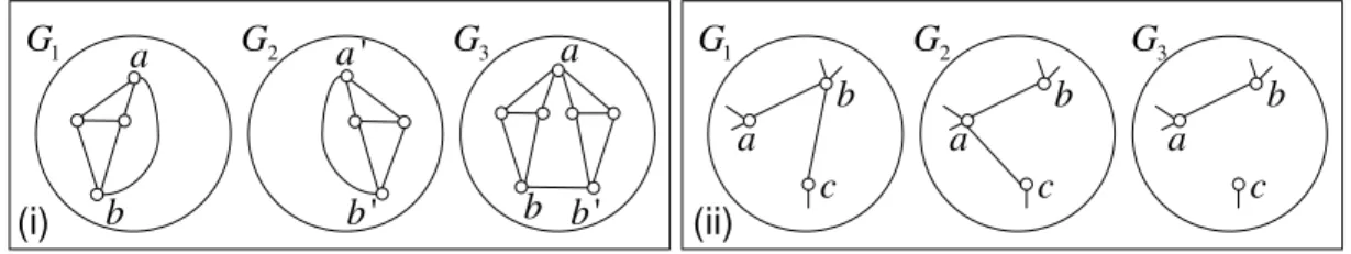
2. Join Rule: Let G1 and G2 be disjoint graphs, a and b adjacent vertices in G1, and a0 and
b0 adjacent vertices in G2. Construct a graph G3 from G1 ∪G2 as follows. First, remove
edges (a, b) and (a0, b0); then add an edge (b, b0); lastly, contract verticesaanda0 into a single vertex. (See Fig. 1(i))
3. Contraction Rule: Contract two nonadjacent vertices into a single vertex, and remove any resulting duplicated edges.
Vertex/Edge Introduction Rule implies that if a subgraph ofGhas a construction,Galso has a construction. Rules 1 and 2 increase vertices and/or edges, but Rule 3 reduces vertices and edges,
(i) (ii) a 1 G G2 a' G3 b b' a ' b b 1 G G2 G3 b c a a a b b c c
Figure 1: (i)Join Rule (ii)Edge Elimination Rule
thus the construction may not be polynomially bounded or the number of construction steps may not be bounded by polynomial in |G|. There is another version of the Haj´os calculus, denoted by HC. The system HC has the same set of initial graphs, as well as Rules 1 and 3 of the Haj´os calculus, but Rule 2 is replaced by the following rule:
4. Edge Elimination Rule: LetG1 andG2 be two graphs with common vertex set{a, b, c, . . .}
which are identical except thatG1 contains edges (a, b) and (b, c) and not (a, c), whereasG2
contains edges (a, b) and (a, c) and not (b, c). Then fromG1 andG2, we can construct a graph
G3 that is identical to G1 but does not contain (b, c) (See Fig. 1(ii)).
LetC andC0
be two graph calculus systems, thenCp-simulates C0
if there is a polynomial-time computable functionf so that for all graphsG, ifσis a graph construction ofGinC0
, then f(σ) is a graph construction ofGin C. C and C0
arep-equivalent ifC p-simulates C0
andC0
p-simulates C. Proposition 1 ([21]). HC isp-equivalent to the Haj´os calculus.
3
Planar Haj´
os Calculus
Now we introduce our new system, the planar Haj´os calculus. Suppose that a sequence of graphs
G1, G2, . . . , Gm satisfies the following conditions: (i) All Gi are planar. (ii) Each Gi is K4 or is
constructed from previous graph(s) by one of the three rules of HC. Then we say that Gm is
constructed by planar HC or PHC. Note that Rules 1 and 3 (but not Rule 4) may violate the planarity of the graph. So, the definition is equivalent to the following: When we introduce a new edge between verticesaand bofGi, then there must be a planar embedding ofGi such that aand b are on the same face. When we apply Contraction Rule between vertices a and b of Gi, then
there must be a planar embedding of Gi such that for all vertices x being adjacent to a, vertex b
is also adjacent to xorb and xare on the same face.
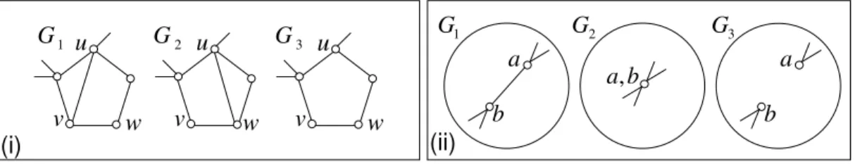
In some cases, this planarity restriction is quite annoying. Fig. 2(i) shows a simple example. Suppose that we wish to remove the chord (u, v) to make a face of size five in some planar graph as
G1. Then what we would do is to construct another planar graph asG2and apply Edge Elimination
Rule to obtainG3. One should notice, however, that this can be done because we can draw the other
cord (u, w) without violating planarity and that it is no longer obvious if such a chord elimination is still possible for a face of sizefour.
To overcome this difficulty, we introduce a new Edge Elimination Rule.
5. Edge Elimination Rule II: Let G1 be a graph with vertices {a, b, . . .} that contains an
edge (a, b), and G2 be the same graph asG1 except that verticesaand b(after removing the
edge between them) are contracted. Then fromG1 andG2, we can construct a graphG3 that
(i) (ii) u v w 1 G G2 u G3 u v w v w 1 G G2 G3 b a , a b a b
Figure 2: (i)Removing chords (ii)Edge Elimination Rule II
To make the difference clear, Rule 4 is called Edge Elimination Rule I from now on. This rule obviously keeps non-3-colorability and the following fact shows that it is at least as powerful as the Rule 4. See Fig. 1(ii). Let G4 be a graph obtained by contracting an edge (a, c) of G1. Then
we get G3 from G2 and G4 by Edge Elimination II, meaning Rule 4 can be simulated by Rules 5
and 3. (Consequently, notice that Rules 1, 3 and 5 are a new complete system for generating non-3-colorabe graphs.)
Thus adding Rule 5 to PHC may seem to increase the power of the system, but we can prove that this is not the case, i.e., Rule 5 can be simulated by PHC in polynomial steps, as shown in Lemma 3 of section 5. It turns out that the new rule is quite convenient for dealing with faces of size four, which plays an important role in the rest of the paper.
ObviouslyPHC is sound, i.e., all graphs generated byPHC are non-3-colorable (planar) graphs. LetLP HC be the set of such graphs generated byPHC. What we want to prove to attain our goal is thatHCgenerates all non-3-colorable graphs in polynomial steps if and only ifPHC generates all graphs in LP HC in polynomial steps. Thus LP HC does not necessarily contain all non-3-colorable planar graphs or PHC is not necessarily complete. In fact there is no obvious extension of the proof for the HC’s completeness to the proof for the PHC’s completeness. Fortunately, however, the proof of our main theorem immediately implies the completeness ofPHC, which is an important by-product of this paper.
4
Planarization of a Graphs
Intuitively speaking, our main theorem clams that PHC is as powerful as HC. To prove this, the natural approach is to develop a simulation of HC by PHC: Suppose that a planar graph G can be generated by HCby a sequence of (maybe non-planar) graphsG1, G2, . . . , Gm=G. Then what
we do is to define planar graphs H1, H2, . . . , Hm =Gsuch that each Hi is “similar” to Gi and it
can be generated byPHC from previousHj’s (j < k) in polynomial steps. To define the similarity,
we can use the so-called the Crossover Gadget; [10] showed that for a given (non-planar) drawing
b
Gof a graphG, we can construct a planar graphH such thatGis 3-colorable iffH is 3-colorable. (A graph is drawn in the plane in such a way that each vertexvis represented by a point and each edge (u, v) by a continuous line connecting the two points corresponding tou and v.)
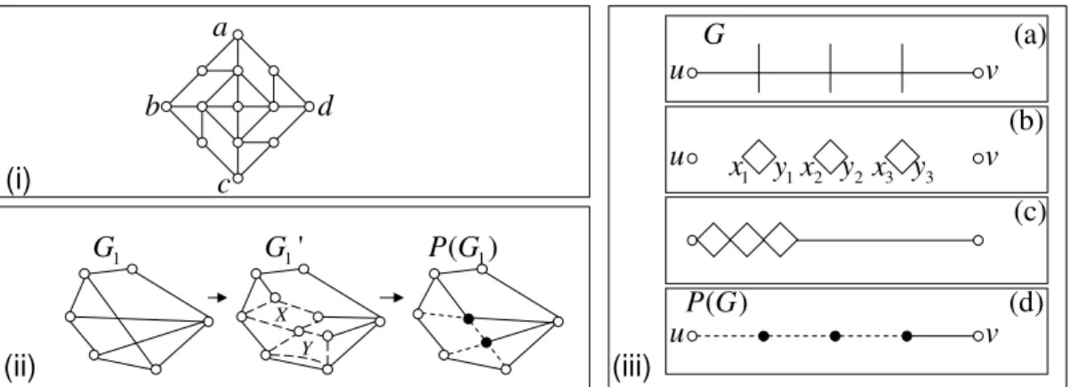
Definition 1 ([10]). The Crossover Gadget, denoted by 3, is a planar graph given in Fig. 3(i). Outer vertices a and c (b and d, also) are said to be opposite. One can easily see that opposite vertices must have the same color in any proper 3-coloring.
Using this gadget, the non-planar drawing of G1 of Fig. 3(ii) is converted to a planar graphG01,
whereX andY are Crossover Gadgets. More formally:
Definition 2. For a given drawing G of a graph, its planarization P(G) is a planar graph con-structed by the following procedure: (i)Each crossing ofGis replaced by a3(see Fig. 3(iii)(a)–(b)).
(i) (iii) (ii) a b c d u 1 x x2 x3 v 1 y y2 y3 G ( ) P G (a) (b) (c) (d) u u v v 1 G G1' P G( 1) X Y
Figure 3: (i)Crossover Gadget (ii)Example of Planarization (iii)Planarization Process (ii)Letu, x1, y1, . . . , xk, yk, v be vertices corresponding to edge(u, v) inG, wherexi andyi are pairs
of opposite vertices of each introduced3’s, and consider pairs of vertices(u, x1),(y1, x2), . . . ,(yk, v).
Draw an edge for exactly one of these k+ 1 pairs and contract all the others. (See Fig. 3(iii)(c)). The structure as shown in Fig. 3(iii)(c) is called an extended edge (or E-edge for short) and is also illustrated as in Fig. 3(iii)(d), where dotted lines show contractions and •’s show Crossover Gadgets. Fig. 3(ii) shows such a representation of P(G1).
5
Basic Tools of
PHC
In this section we will prove a key lemma (Lemma 1). Suppose that there is a sequenceG1, G2, . . . , Gm
of planar graphs such that (i)G1 is any (non-3-colorable, often omitted) planar graph (called an
axiom) (ii)For each 2 ≤ i ≤ m, Gi is K4 or can be derived from previous graphs by PHC in
polynomial steps. Then we writeG1
∗
⇒Gm. We also write G1, G2
∗
⇒Gm if we need two axioms.
Lemma 1 (Redrawing). Suppose G1 and G2 are two drawings of the same (not necessarily
planar) graph. Then P(G1)
∗
⇒P(G2) in poly(|G1|) +|G2|) steps.
The following lemmas provide convenient tools to prove G1
∗
⇒G2 and to prove Lemma 1.
Lemma 2 (Triangle Elimination). Let G1 be a planar graph having a vertex v with degree at
most two, and G2 be the (obviously planar) graph obtained by removing v and its outgoing edges
from G1. Then G1
∗
⇒G2 in polynomial steps.
Proof. Ifv’s degree is zero, all we have to do is to merge it to a nearby vertex. Suppose thatv’s degree is one. Then v has only one edge, (u, v), and if u is adjacent to another vertexw, then we can contractvandw. Otherwise, contractuand vwithu0 andv0 such that an edge exists between them (If no suchu0 and v0 exist, then the graph would be 3-colorable).
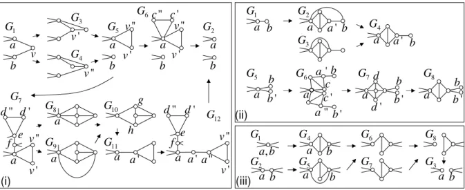
So, we can restrict ourselves to the case thatvis of degree two. See Fig. 4(i). Letaandbbe the two vertices adjacent tov and there may or may not be an edge betweenaandb. We add vertices and edges as G3 and G4, and get G5 by Edge Elimination I. Now we are going to remove triangle
a, v0, v00 (vertices v0, v00 and the three edges). This is the main part of this lemma and therefore we call this procedure Triangle Elimination. Ifais a part of another trianglea, c0, c00
as shown inG6,
(i) (ii) (iii) v a b 1 G G3 4 G 5 G G2 ' v '' v " c c' ' d " d 6 G 7 G 8 G 9 G 10 G 11 G 12 G ' a a" e f g h a b a b ' v '' v v'' ' v a a a a a' f e ' d " d ' v '' v ' v '' v 1 G G2 b a a' ' b c ' c " a d' d a b a a' b 3 G 4 G a b a ' a b ' b a b ' b a b ' b 5 G G6 G7 G8 , a b a b a b a b a b 1 G 2 G G3 4 G 5 G 6 G 7 G 8 G a a b
Figure 4: (i)Triangle Elimination (ii)Equality Introduction (iii)Edge Elimination II
Otherwise, we look for a triangle near a (say, e, d0, d00 in G7) which is guaranteed to exist
somewhere since the underlying graph is a non-3-colorable, planar graph [12]. Then we continue to change the graph into asG8 andG9 by Vertex/Edge Introduction thenG10by Edge Elimination I,
and G11 by Contraction (of vertices g and h), which allows us to introduce one extra edge (a, a0)
to the triangle. By repeating the same procedure, we can get another extra edge (a0, a00) as inG12.
Now we can contract a0 and f, a00 and e, v0 and d0, and v00 and d00. Extension to the general
case is straightforward. ¤
Lemma 3 (Simulation of Edge Elimination II). Edge Elimination II can be simulated by
PHC in polynomial steps.
Proof. For the simulation, we first need a tool, what we callEquality Introduction (see Fig. 4(ii)). Consider an arbitrary vertex, say, a, as in G5. Our goal is to split a into two vertices a and a0
and to put two triangles with a shared edge between them asG8. The edges from aare arbitrarily
divided into from aand from a0 whenever the resulting graph is a planar graph. If the number of such divided edges froma0 (or from a) is one, seeG1 ∼G4. From G1 toG2, a simple Vertex/Edge
Introduction is enough,G3 can be constructed from K4, andG4 is due to Edge Elimination I from
G2 and G3. If there are two edges from a0, see G5 ∼G8 (The case that there are three or more
edges froma0 is similar and omitted). Repeat the above procedure twice to getG6 and contracta0
and a00 andc and c0 to getG7. Finally G8 can be obtained by contracting d and d0.
Now the simulation of Edge Elimination II goes like Fig. 4(iii). From G1 toG4 is by Equality
Introduction,G2toG5by Vertex/Edge Introduction,G6(and alsoG7 =G6) by Edge Elimination I.
G8 is obtained by Edge Elimination I and finally we get G3 by Triangle Elimination. ¤
Lemma 4 (Crossover Construction). Crossover Gadget G1 as shown in Fig. 5 can be
con-structed by PHC.
Proof. First we get X(2) by Equality Introduction toK4. ThenG3, G4, G6, G8, G9 are obtained
from X(2) by (after contracting c and f for G3, G6 and G9) Vertex/Edge Introduction. For
f c 1 G 2 G G3 4 G (2) X a b c d e f g a b g d e f c g a b c d f e 5 G 6 G 7 G 8 G 9 G a b d e g a b c d e f g a b c d e f g
Figure 5: Crossover Construction
used to show corresponding vertices. All the remaining graphs are obtained by Edge Elimination II which can now be used by Lemma 3. For example, we getG2 from G3 and G4 sinceG3 is a graph
obtained by contracting e and f of G4 (edge (e, f) of G4 is given as a bold line in the figure and
similarly for the others). ¤
Lemma 5 (Crossover Introduction). As Equality Introduction, a Crossover Gadget can be added. See Fig. 6(i).
Proof. From G1 to G4, we just use Vertex/Edge Introduction (the added part is a Crossover
Gadget whose two opposite vertices are merged). G3 is by Crossover Construction that is possible
by Lemma 4. Use just Vertex/Edge Introduction to makeG5similar to the whole underlying graph.
Finally G2 is obtained by Edge Elimination II. ¤
(i) (ii) a b c d e f g , b d , , a b d h i j k 1 G 2 G 3 G G4 G5 6 G 7 G G8 9 G G10 a b c b d , b d a c a , b d a d a c , , a b d a b d c , , a b d j e , a b a b, 1 G G2 3 G 4 G 5 G a b a b a b
Figure 6: (i)Crossover Introduction (ii)Crossover Elimination
Lemma 6 (Crossover Elimination). Let a, b, c and d be four outer vertices of a Crossover Gadget and b and d be opposite. Moreover c is free, i.e., c is not connected to any vertices except those in the Crossover Gadget. Then this Crossover Gadget can be removed, i.e.,banddare merged
into a single vertex, a also remains, but all the other vertices and edges of the Crossover Gadget can be removed in polynomial steps. Namely, G1 is changed to G2 in Fig. 6(ii).
Proof. Contracts vertices aand f (and three others similarly) to get G3, and remove triangles
to getG4. Contractband d(this is possible sincec has no edges other than the three edges of the
gadget). Two Triangle Eliminations to get G6. As a different direction from the original graph,
mergee and g (and three others) to get G7, and contract c toh,b toaand d toato get G8. G9
is obtained by applying two Contractions, i and j and k and l, G10 is by Triangle Elimination.
Finally use Edge Elimination II fromG6 and G10 toG2. ¤
Now we are ready to prove Lemma 1.
Proof of Lemma 1. LetG1 andG2be two drawings of the same graphG. We are going to show
thatP(G1)
∗
⇒P(G2) can be done (in polynomial steps) by the following algorithm. For exposition,
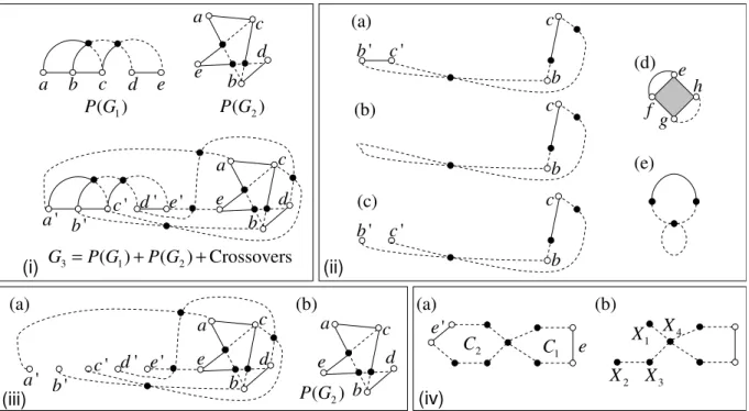
we use the example in Fig. 7(i) (recall that a Crossover Gadget is represented by •). Note that vertices of the same label inP(G1) and P(G2) correspond to the same vertex ofG.
Step 1 P(G2) is just added toP(G1) (by Vertex/Edge Introduction).
Step 2 Connect each pair of two vertices of the same label by using Crossover Gadgets as shown in Fig. 7(i). Let this new graph be G3. Note that we may need two or more Crossover Gadgets
to connect a single pair of vertices to maintain newly created crossings but it is easily seen that we can bound the total number of those Crossovers by a polynomial in |P(G1)|+|P(G2)|. Each
vertex label inP(G1) is changed from `to`0 (atoa0,btob0, etc., as in the Figure).
Step 3 We now delete all the edges of P(G1) one by one: Suppose that we want to delete edge
(b0, c0). Then all we have to do is to create a graph which is exactly the same as G3 except that
verticesb0 andc0 are contracted (and then Edge Elimination II can be used to remove the edge). To to so, consider the cycle consisting of E-edge (b, c), edge (b0, c0
), and Crossover Gadgets connecting
b and b0, and c and c0 (Fig. 7(ii)(a)). Note that the cycle is “twisted” and one can easily see that at most one twist is enough for each cycle (The following procedure becomes easier if there is no twist).
Now see Fig. 7(ii)(b). Our goal is to construct G3 with contracted b0 and c0. We start with a
planar graph in Fig. 7(ii)(d) consisting of a single Crossover Gadget (let its outer vertices bee, f, g
and h, e and g and f and h are opposite) such that e and f are connected by a single edge and
g and h are contracted. Obviously this graph is non-3-colorable, and it can be generated by PHC
in finite steps. (See Fig. 8. G1 is just by Crossover Construction. G2 is obtained from G1 by two
contractions between b and c and d and c. G3 is obtained from G1 by contracting c and d and
adding an edge (a, b). Note that labelsatodofG1are used to show corresponding vertices. Finally
we getG4, which is exactly the same graph in Fig. 7(ii)(d), fromG2 andG3 by Edge Elimination II
since G2 and G3 are the same graph if the bold (a, c) in G3 is contracted.) We then insert two
Crossover Gadgets at vertices eand f and get Fig. 7(ii)(e), which is exactly the same as (b). Now we add vertices and edges to make it the same as G3 excepting the contractedb0 and c0. Let this
new graph beG03 and apply Edge Elimination II to delete the edge (b, c) fromG3 as in Fig. 7(ii)(c).
Repeat this procedure to remove all the edges of P(G1) part. Thus we obtain the graph as in
(i) (ii) (iv) (iii) 2 ( ) P G 3 ( 1) ( 2) Crossovers G =P G +P G + 1 ( ) P G a b c d e ' a b' c' ' d e' a b c d e a c b e d (a) (b) (c) ' b c' b c b c b c ' b c' ' a b' c' ' d e' a c b e d (a) ' e 1 C 2 C e X1 3 X 2 X 4 X (a) (b) a b c d e (b) 2 ( ) P G (e) e f g h (d) Figure 7: Redrawing 1 G , , b c d a b a c d , c d a b 2 G G3 G4
Figure 8: Construction of the Gadget in Fig. 7(ii)(d)
Step 4 Remove all the Crossover Gadgets excepting those within P(G2) to get Fig. 7(iii)(b).
Recall that when we remove the Crossover Gadgets, one by one, we need to find a Crossover Gadget such that at least one of its outer vertices is free. To see this is always possible until all the Crossover Gadgets disappear, see the cycle as in Fig. 7(iv)(a). Note that the cycle is twisted and we can regard that it consists of two cycles, C1 and C2, each including an edge (e ore0). Suppose
that edgee0 is removed at step 3. Then the cycleC2is “cut”, as shown in Fig. 7(b). Thus Crossover
Gadgets X1 and X2 have free outer vertices and can be removed. Then X3 has a free vertex and
is removed. Then X4 can be removed and the second cycle C1 is also cut and Crossover Gadgets
included this cycle can also be removed similarly. This complete the proof for P(G1)
∗
⇒ P(G2). It is not hard to see that the procedure needs
6
Main Theorem
We are now ready to prove our main theorem.
Theorem 1. PHC is polynomially bounded iff so is HC.
Proof. We first prove the if-part. Suppose that HC is polynomially bounded for any (non-3-colorable) graph. Then it is obviously polynomially bounded for any (non-3-(non-3-colorable) planar graph
G. Hence there is a sequence of (not necessarily planar) graphs
G1, G2, . . . , Gm =G
such that eachGi is (i) K4 or (ii) for some j < i,Gi is generated fromGj by Rule 1 (Vertex/Edge
Introduction) or Rule 3 (Contraction) of HC or (iii) for some j, k < i, Gi is generated from Gj
and Gk by Rule 4 (Edge Elimination I) of HC, all in time polynomial in |G|. For this sequence of
graphs, we prove that there exists a sequence of drawings
H1, H2, . . . , Hm, H
such that:
(i) Hi is a (maybe non-planar) drawing ofGi andH is an arbitrary planar drawing ofG.
(ii) For each 1≤ i≤ m, K4
∗ ⇒ P(Hi) or for some j < i, P(Hj) ∗ ⇒ P(Hi) or for some j, k < i, P(Hj), P(Hk) ∗
⇒ P(Hi), all in polynomial steps. Here, “polynomial” means polynomial
in |P(Hj)|+|P(Hk)|, which also means polynomial in |G| since |P(Hi)| is bounded by a
polynomial in|Gi|for alli and|Gi|is bounded by a polynomial in |G|by assumption.
(iii) P(Hm)
∗
⇒H in polynomial (the same as above) steps.
Now we shall prove that for eachGiandG, there exists the correspondingHiandHthat satisfy
these three conditions by induction, which obviously means that any non-3-colorable planar graph (G) can be generated by PHC in a polynomial number of steps. If i= 1, then G1 must be aK4.
Then we can selectH1 as the planar drawing of K4, and obviouslyK4
∗
⇒P(H1) in 0 steps.
For Gi (i≥2), there are several cases:
Case 1 Gi is aK4. Completely the same as above.
Case 2 Gi is obtained from Gj (j < i) by Vertex/Edge Introduction. By induction hypothesis Hj is a proper drawing ofGi. To add an vertex, just add one in anywhereHj to obtain Hi, which
is obviously a proper drawing ofGi and satisfies the three conditions. If an edge is added between v1 and v2 of Gj, then we draw an edge between the corresponding vertices of Hi, which is also a
proper drawing of Gi. For P(Hi) we may need to add Crossover Gadgets along the added edge.
The number of such Crossover Gadgets is at most the number of already existing (E-)edges and thus a polynomial number of steps suffice forP(Hj)
∗
⇒P(Hi).
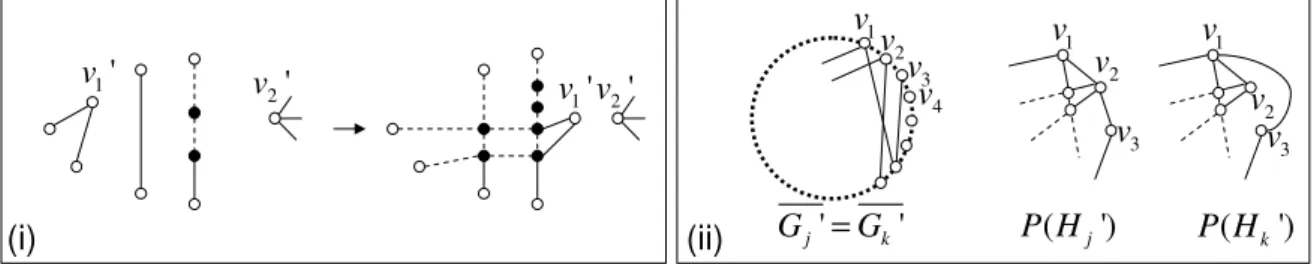
Case 3 Giis obtained fromGj(j < i) by contracting two vertices,v1andv2. To obtainHi, we just
“drag”v10 tov 0 2, wherev 0 1 andv 0
2 correspond to v1 and v2 ofGj, respectively. ForP(Hj)
∗
⇒P(Hi),
see Fig. 9(i). Again we dragv0
i into the facev
0
2 is on inP(Hj), where we may need to add (at most
a polynomial number of) Crossover Gadgets as shown in Fig. 9(i). After that the two vertices are contracted in a single step. Thus the wholeP(Hj)
∗
(i) (ii) 1' v 2' v 1' v v2' 2 v 1 v 4 v3 v ' ' j k G =G P H( j') P H( k') 1 v v1 2 v 2 v 3 v 3 v
Figure 9: (i)Case 3 (ii)Case 4
Case 4 Gi is obtained from Gj and Gk (j, k < i) by Edge Elimination I. Let v1, v2 and v3 be
important vertices such that edge (v1, v2) exists both in Gj and Gk, edge (v2, v3) only in Gj, edge
(v1, v3) only inGk. All the other parts ofGj andGkare the same. LetG0j (G0k, respectively) be the
graph obtained from Gj (Gk, respectively) by removing the above two edges (v1, v2) and (v2, v3)
((v1, v2) and (v1, v3), respectively). By definition, G0j and G0k are the same graph and have the
same drawing ¯G0j and ¯G0k. This uniqueness of the drawing is important when we handleP(Hj0) and
P(Hk0) later, and for such a drawing, we can use for instance the following method. The vertices are placed on a circle in the clockwise order of v1, v2, v3, . . . , vn, and each edge is drawn as a straight
line (See Fig. 9(ii)).
Now we put the removed two edges back to each of ¯G0j and ¯G0k, obtaining Hj0 and Hk0, where (v1, v2) and (v2, v3) are drawn as straight lines, but (v1, v3) is drawn as going around the outside of
v2 without any crossings. Their planarizationP(Hj0) andP(Hk0) are given in Fig. 9(ii). Apparently
Hj and Hj0 are drawings of the same graph Gj and so are Hk and Hk0. Hence, by Lemma 1, P(Hj)
∗
⇒ P(Hj0) and P(Hk)
∗
⇒ P(Hk0), both in polynomial steps. Since P(Hj0) and P(Hk0) are exactly the same graph excepting edge (v2, v3) inP(Hj0) and (v2, v3) in P(Hk0), we can apply Edge
Elimination I to get the graph P(Hi). Because of the drawing rule above mentioned, we can
determineHi from P(Hi) uniquely, which is obviously a drawing ofGi.
Case 5 Deriving ofHfromP(Hm). Recall thatHis a planar drawing ofGandHmis a (possibly
non-planar) drawing of Gm, but since Gm and G are the same graph, H and Hm are drawing of
the same graph. Thus we can use Lemma 1, i.e.,P(Hm)
∗
⇒Hin polynomial steps. This completes the proof of the if-part.
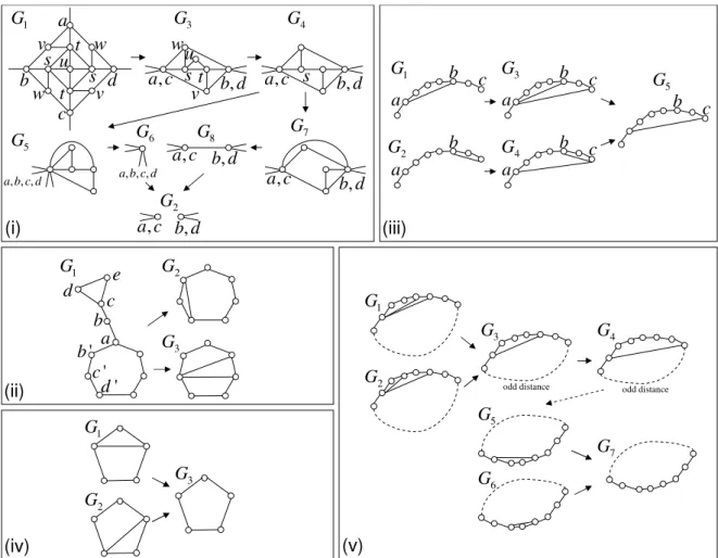
The proof of the only-if part is easier but rather technical. Suppose that PHC is polynomially bounded. Let Gbe any (possibly non-planar) non-3-colorable graph and we denote its reasonable (without too many crossings) drawing also byG. Then the size ofP(G) is bounded by a polynomial and it can be generated by PHC in polynomial steps. In order to show that HC is polynomially bounded, it now suffices to show that G can be derived from P(G) by HC in polynomial steps. Note that this is nothing other than a sequence of Crossover Eliminations. See Fig. 10(i): G1 is a
Crossover Gadget we want to remove. G3 is obtained by Contractions ofaandc,banddand pairs
of vertices labeled by s, t, v, w (recall we do not have to preserve planarity). G4 is by Triangle
Elimination (we need a care as mentioned below). G5 and G7 are by Contractions ofb, d anda, c,
andsandb, d, respectively. G6 and G8 are both by sequences of triangle Eliminations. Finally, G2
is by Edge Elimination II.
Recall that the previous proof for Triangle Elimination needed the fact that any non-3-colorable planar graph has a triangle as a subgraph. In the above derivation, we cannot use this property since the graph may no longer be planar. So, in the following, we redesign the procedure for
Triangle Elimination by assuming that the graph includes a chord-less cycle of odd length. (Any non-3-colorable graph has such a cycle since otherwise the graph is bipartite.) See Fig. 10(ii). By using the same procedure as before, we can make a trianglecde and a “shaft” abcwhich connects the triangle and the odd cycle. Our goal is to remove this triangle and shaft. Recall that we can change the length of shaft arbitrarily.
(i) (ii) (iii) (iv) (v) a b c d s t u v w , b d , a c , , , a b c d 1 G 2 G 3 G G4 5 G G6 G8 G7 t v w a c, b d, w s t u s v s , a c b d, , , , a b c d , a c b d, , a c b d, a ' b c b d ' c ' d e 1 G G2 3 G 3 G 1 G 2 G 1 G 2 G 3 G 5 G 4 G a b c a b c b c a a b b c 1 G 2 G 3 G G4 5 G 6 G 7 G
odd distance odd distance
Figure 10: Crossover Elimination and Triangle Elimination
We have three basic operation: (i)Chord of size three(3-chord). As shown in Fig. 10(ii), we can replace the triangle and shaft by a chord which connects two cycle vertices of distance two (as in G2). This can be done by, for instance, contractingb and b0,c and c0, d and d0, and e and
b0. (ii)Inner triangle. As shown in G3, we can replace the triangle and chord by a inner triangle
consisting of one cycle edge + two chords by a procedure similar to (i). (iii)Chord Shift. See Fig. 10(iii). Suppose that the triangle and shaft is replaced by chordab(G1). Then we also apply
3-Chord to the original graph and get G2. G3 and G4 are obtained by Vertex/Edge Introduction
from G1 and G2 respectively. Then Edge Elimination I from G3 and G4, we can getG5 where the
one endpoint of the chord is “shifted” two positions on the cycle.
Now the triangle and shaft can be removed as follows: If the cycle is a triangle then we are done as before. If the cycle is of size five, then see Fig. 10(iii). By 3-chord, we can make G1 and
G2, followed by Edge Elimination I. Suppose that the cycle is of size seven or more. See Fig. 10(v).
G1 is obtained by Inner Triangle, where two chords connect vertices of distance three and distance
Notice that inG3 the chord connects two vertices whose lower-half distance is odd and this is also
true in G4. Repeating Chord Shift, we can reach, from the original graph, G5 where the chord
connects two cycle vertices of distance three. G6 is obtained by 3-Chord and finallyG7 is obtained
by Edge Elimination I.
Thus Triangle Elimination is still possible for non-planar non-3-colorable graphs, completing
the proof of the only-if part. ¤
If we allow arbitrary steps for generation, the above proof claims that if a planar non-3-colorable graphGis generated byHC, then so is byPHC. Since the former is complete, we have the following theorem:
Theorem 2. PHC is complete.
7
Concluding Remarks
Recall that our final goal is to find a hard example forPHC. Note that if the generation system is more deterministic, or application of each rule is more restricted, then it is usually better to prove lower bounds. In this sense, we should seek even more restricted graph calculus whose complexity is p-equivalent to that of PHC. We already have candidates, for example, generation systems for degree-restricted non-3-colorable planar graphs.
References
[1] M. Ajtai. The complexity of the pigeonhole principle. Combinatorica, 14(4):417–433, 1994. [2] K. Appel and W. Haken. Every planar map is four colorable. Part I. Discharging. Illinois
J. Math., 21:429–490, 1977.
[3] K. Appel, W. Haken and J. Koch. Every planar map is four colorable. Part II. Reducibility. Illinois J. Math., 21:491–567, 1977.
[4] S. R. Buss, D. Grigoriev, R. Impagliazzo and T. Pitassi. Linear gaps between degrees for the polynomial calculus modulo distinct primes.J. Comput. Syst. Sci., 62(2):267–289, 2001. [5] P. Beame and T. Pitassi. Propositional proof complexity. Past, present, and future. Bulletin
of the European Association for Theoretical Computer Science, 65:66–89, 1998.
[6] S. A. Cook and R. A. Reckhow. The relative efficiency of propositional proof systems. J. Symb. Log., 44(1):36–50, 1979.
[7] S. Dash. An exponential lower bound on the length of some classes of branch-and-cut proofs. Mathematics of Operations Research, 30(3):678–700, 2005.
[8] Z. Galil. On the complexity of regular resolution and the Davis-Putnam procedure. Theor. Comput. Sci., 4(1):23–46, 1977.
[9] M. R. Garey and D. S. Johnson. Computers and Intractability. A Guide to the Theory of NP-Completeness. W. H. Freeman and Company, New York, 1978.
[10] M. R. Garey, D. S. Johnson and L. J. Stockmeyer. Some simplified NP-complete graph prob-lems.Theoretical Computer Science, 1(3):237–267, 1976.
[11] M. Grigni, E. Koutsoupias and C. H. Papadimitriou. An approximation scheme for planar graph TSP. InProc. of FOCS 1995, pp. 640–645, 1995.
[12] H. Gr¨otzsch. Ein Dreifarbensatz f¨ur dreikreisfreie Netze auf der kugel.Wiss. Z. Martin Luther Univ. Halle-Wittenberg, Math. Nat. Reihe, 8:109–120, 1959.
[13] G. Haj´os. ¨Uber eine Konstruktion nicht n-f¨arbbarer Graphen. Wissenschaftliche Zeitschrift der Martin-Luther-Universit¨at Halle-Wittenberg, A 10:116–117, 1961.
[14] A. Haken. The intractability of resolution.Theor. Comput. Sci., 39:297–308, 1985.
[15] J. E. Hopcroft and J. K. Wong. Linear time algorithm for isomorphism of planar graphs (Pre-liminary Report). InProceedings of the 6th annual ACM symposium on Theory of Computing, pp. 172–184, 1974.
[16] K. Iwama and T. Pitassi. Exponential lower bounds for the tree-like Haj´os calculus. Informa-tion Processing Letters, 54(5):289–294, 1995.
[17] J. Kraj´ıˇcek. Bounded Arithmetic, Propositional Logic, and Complexity Theory. Cambridge University Press, New York, 1995.
[18] J. Kraj´ıˇcek, P. Pudl´ak and A. Woods. Exponential lower bounds to the size of bounded depth Frege proofs of the pigeonhole principle.Random Structures and Algorithms, 7(1):15–40, 1995. [19] R. J. Lipton and R. E. Tarjan. Applications of a planar separator theorem.SIAM Journal on
Computing, 9(3):615–627, 1980.
[20] T. Pitassi, P. W. Beame and R. Impagliazzo. Exponential lower bounds for the pigeonhole principle.Computational Complexity, 3:97–140, 1993.
[21] T. Pitassi and A. Urquhart. The complexity of the Haj´os calculus.SIAM Journal on Discrete Mathematics, 8(3):464–483, 1995.
[22] P. Pudl´ak. Lower bounds for resolution and cutting planes proofs and monotone computations. J. of Symb. Logic, 62(3):981–998, 1997.
[23] P. Pudl´ak. The lengths of proofs. In S. R. Buss (ed.), Handbook of Proof Theory, Elsevier, pp. 547–637, 1998.
[24] A. A. Razborov. Lower bounds for propositional proofs and independence results in bounded arithmetic. InProc. of ICALP 1996, pp. 48–62, 1996.
[25] N. Segerlind. The complexity of propositional proofs. The Bulletin of Symbolic Logic, 13(4):482–537, 2007.
[26] C. S. Tseitin. On the complexity of derivation in the propositional calculas. In A. O. Slisenko (ed.),Studies in Constructive Mathematics and Mathematical Logic, Part II, 1968.
[27] A. Urquhart. The complexity of propositional proofs.Bulletin of Symbolic Logic, 1(4):425–467, 1995.