Experimental Twin-Field Quantum Key Distribution Through
Sending-or-Not-Sending
Yang Liu,1, 2, 3 Zong-Wen Yu,4, 5 Weijun Zhang,6 Jian-Yu Guan,1, 2 Jiu-Peng Chen,1, 2 Chi Zhang,1, 2 Xiao-Long Hu,4 Hao Li,6 Teng-Yun Chen,1, 2 Lixing You,6 Zhen Wang,6 Xiang-Bin Wang,2, 3, 4 Qiang Zhang,1, 2 and Jian-Wei Pan1, 2
1Shanghai Branch, National Laboratory for Physical
Sciences at Microscale and Department of Modern Physics,
University of Science and Technology of China, Shanghai 201315, P. R. China
2Shanghai Branch, CAS Center for Excellence and Synergetic
Innovation Center in Quantum Information and Quantum Physics, University of Science and Technology of China, Shanghai 201315, P. R. China
3Jinan Institute of Quantum Technology,
Jinan, Shandong 250101, P. R. China
4State Key Laboratory of Low Dimensional Quantum Physics,
Department of Physics, Tsinghua University, Beijing 100084, P. R. China
5Data Communication Science and Technology
Research Institute, Beijing 100191, P. R. China
6State Key Laboratory of Functional Materials for Informatics,
Shanghai Institute of Microsystem and Information Technology, Chinese Academy of Sciences, Shanghai 200050, P. R. China
Abstract
Channel loss seems to be the most severe limitation to the application long distance quantum key distribution in practice. The idea of twin-field quantum key distribution can improve the key rate from the linear scale of channel loss in the traditional decoy-state method to the square root scale of the channel transmittance. However, the technical demanding is rather tough because it requests single photon level interference of two remote independent lasers. Here, we adopt the technology developed in the frequency and time methology field to lock two independent lasers’ wavelengths and utilize additional phase reference light to estimate and compensate the fiber fluctuation. Further with a single photon detector with high detection rate, we demonstrate the real optical fibre experimental results of twin field quantum key distribution through the sending-or-not-sending protocol, which is fault tolerant to large misalignment error. We obtain the key rates under 4 different distances, 0km, 50 km, 100km and 150km. Especially, the obtained secure key rate at 150 km is higher than that of the measurement device independent QKD.
Introduction.— Although quantum key distribution(QKD) can in principle offer secure private communication [1–7], there are still some technical limitations in practice for long distance quantum communication. The most severe one is perhaps the channel loss given that a quantum signal cannot be amplified. Much efforts have been made towards the longer-distance QKD. Theoretically, the decoy-state method [8–10] can improve the key rate of coherent-state based QKD from the quadratic scale of channel transmittance to the linear scale, as what behaves of a perfect single-photon source. There, the method can beat the photon-number-splitting attack to the imperfect source and the coherent state is used as if only the single-photon pulses were used for key distillation and hence it can reach a key rate in the linear scale of channel loss, as the perfect single-photon source does.
Motivated to a longer secure distance for practical QKD, a remarkable theoretical progress, the twin-field QKD [11] was proposed to improve the key rate to the scale of square root of channel transmittance. It shows that, the coherent-state source can actually be an advantage to the single-photon source because the post-selection of phase coherence of the twin fields from Alice and Bob can possibly make the secure QKD with the encoding state of single-photon and vacuum, and their linear super-positions. Possibly, This can achieve a key rate of square root scale of channel transmittance, and can by far break the known distance limit of existing protocols in practical QKD [12–20]. However, considerable jobs still have to be done to really make so. First, it is theoretically challenging on how to making use of both the phase information post selection and the traditional decoy-state method. Second, it is technically demanding to make the long distance single-photon in-terference precisely. Towards this goal, the sending-or-not-sending (SNS) protocol [21] was proposed. It proposes a small probability of sending for both Alice and Bob, and then use sending and not-sending decisions for the bit value encoding in Z-basis with the effective heralding events announced by Charlie. InX-basis, an effective event needs not only Char-lie’s announcement of only one detector clicking, but also the phase difference of Alice and Bob’s private phase shifts to be in the phase slice set by the protocol. In this way, as shown in[21] one can continue to use the tagged model and the conventional decoy-state method in the protocol. Also, since the protocol uses the almost error-free Z-basis for bit value encoding, it can tolerate a high error rate in X-basis.
Here we report an experimental demonstration of TFQKD through SNS protocol (SNS-TF-QKD) over real optical fibre.
Protocol.—We implement the SNS-TF-QKD protocol [21] by the practical 4-intensity protocol [22]. Each party exploits four different intensities 0, µ1, µ2 and µz. Alice and Bob
randomly choose X-basis and Z-basis with probabilities pX and 1−pX respectively. In
X-basis, both Alice and Bob prepare and send the decoy pulses. They each take a phase shift
θA, θB privately to the pulse to be sent out. An event in Z-basis is regarded as an effective
event if Charlie announces only one detector clicking. For an effective event in X-basis, we need an extra phase-slice condition to reduce the observed errors in the basis. Without a reasonable phase-slice condition, the observed errors in X-basis can be too much larger than the actual phase-flip error rate in Z-basis. Note that Charlie does not have to be honest and whatever she announces does not undermine the security. But if Charlie wants to make a good key rate, he will have to try to make a faithful announcement on everything. An error in X-basis is defined as Charlie’s announcement of a click of right detector (left detector) associated with an effective event in X-basis where the phase difference of the pulse pair from Alice and Bob would provably cause a left (right) clicking at Charlie’s measurement set-up. A Z-basis effective event that Alice (Bob) has decided sending and Bob (Alice) has decided not-sending corresponds to a bit value 1 (0). An encoding error in Z-basis is counted for an effective event corresponding to the situation that both of Alice and Bob had decided sending or both of them had decided sending. Since the sending or not-sending decisions correspond to the secret key, they cannot announce all of them for the Z-basis effective events. They can announce a random subset of them and deduce the error rate in Z-basis. The errors in X-basis are used to estimate eph1 , the phase-flip error rate of those single-photon effective events in Z-basis. To know the errors in X-basis, Alice and Bob need to announce the basis information and the intensities of X-basis pulses after Charlie’s announcement, and also the phase-shift information to each sent-out pulses in X -basis. Explicitly, in theX-basis, they randomly choose the vacuum sources and two coherent sources with intensities µ1 and µ2 with probabilitiesp0, p1, p2 respectively. In Z-basis, Alice (Bob) randomly prepares and sends the coherent state with intensity µz with probability
pz and sends nothing else. The value of e ph
1 and s1, the yield of the single-photon effective events in Z-basis can be calculated by the conventional decoy-state method [21, 22]. Detailed calculation is presented in the supplement.
Experiment.— The experimental layout is shown in Fig. 1(a). In Alice’s (Bob’s) lab, an
(b) (a) PM AM ATT PM AM ATT FM PD PD PBS QWP BS BS BS FM BS BS BS PD BS PBS PBS SNSPD1 SNSPD2 PBS PBS Ultrastable Cavity Light Source1 Light Source2 AOM AOM AOM AOM PM 1 1 2 2
FIG. 1. (a) Schematics of our experiment. Alice and Bob use continuous wave (CW) lasers that are frequency locked to each other as the source. The laser is then modulated with a phase modulator (PM) and three intensity modulators (IM1, IM2, IM3) for phase randomization, encoding and the decoy intensity preparation. The pulses are attenuated by an attenuator (ATT) and send out via fiber spools to Charlie. In Charlie’s measurement station, the light from Alice and Bob passes polarization controllers (PCs) and polarization beam splitters (PBSs), and then interfere at a beam splitter (BS). The light is finally measured with superconducting nanowire single photon detectors (SNSPDs). (b) Frequency locking system of Alices and Bob’s lasers. The fiber length between Alice and Bob is set to be the same as the total signal fiber length. AOM: acousto-optic modulator, FM: Faraday mirror, PD: photodiode.
to 16 different phases with a phase modulator (PM). Three intensity modulators (IMs) following the PM are used for encoding. In particular, IM1 modulates the pulse intensity to signal state (µz), decoy states (µ1, µ2) or vacuum state (0); IM2 modulates the intensity of phase reference pulses and the signal states (See Supplemental Materials for details about the phase reference pulse); IM3 further modulates the signal pulses width to 2 ns. All the modulators block the light when the pulse is a “vacuum” state, or the pulse is a “not-sending” state in Z basis. The signal intensities are further attenuated to single photon level with an attenuator before they leave Alice’s (Bob’s) secure zone.
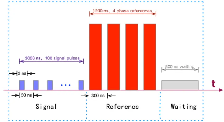
The modulation in Alice’s (Bob’s) lab is controlled by an arbitrary-wave generator (AWG) with pre-generated quantum random numbers. We set a 5µs period in the experiment. In this period, 100 signal pulses are sent in the first 3µswith 30 nsinterval; 4 phase reference
pulses are sent in the next 1.2 µs to estimate the relative phase between Alice’s and Bob’s channel; 0.8 µs vacuum state followed is used as the relaxing time of the SNSPDs. The sampling rate of the AWG is 2 GHz with 14-bit depth, the waveform is then constructed based on the encoding information for each signal and reference pulses.The output signal is amplified to approximately 7 V peak-peak value to drive the modulators. The voltage for different signal states, especially the 16 phases, are characterized before the experiment.
Then, the signals are transmitted from Alice and Bob to Charlie for interference. An interference requires the input signals are identical. Thus, polarization controllers (PCs) and polarization beam splitters (PBSs) are necessary before the polarization maintaining beam splitter (BS). The interference result is detected with superconducting nanowire single-photon detectors (SNSPDs), and is recorded with a high speed Time Tagger.
The main technique challenge in realizing SNS-TF-QKD is to control the phase evolution of the twin field. As pointed out in [11], two sources contribute to the phase difference should be compensated: the first one is the frequency difference between Alice’s and Bob’s sources; the second one is the phase drift in the fiber.
For the phase difference caused by the wavelength difference, we adapt a frequency locking method for compensation. The setup for frequency locking is shown in Fig. 1(b). In Alice’s lab, the seed laser is locked to an ultra-stable cavity using the Pound-Drever-Hall (PDH) technique [23, 24], to decrease the line-width from a few kilohertz to about ten hertz. The light is then split into two parts, one as Alice’s source, the other for locking Bob’s optical frequency. The locking light is further split into two parts, one is reflected by a Faraday mirror (FM) as the local reference, the other is frequency modulated with an acoustic-optic modulator (AOM) and sent to Bob. The fiber length is set to the same as the total length for signal transmission, to show the practicability of the system.
At Bob’s side, a BS and a FM works as a partial reflector for the locking light. a second AOM with fixed frequency shift is inserted before the BS, to distinguish the reflected laser from backscattering and facet reflection noises. The whole setup including Alice’s and Bob’s reflectors is actually a large Michelson interferometer. Thus the phase noise can be measured by detecting the beat pattern at Alice’s photodiode (PD). A PI Servo generate the feedback signal for Alice’s AOM, compensating the phase drift at Bob’s side. Bob then lock his own laser to transmitted laser with a fast AOM feedback and a slow piezoelectric feedback with a large adjustment range. The whole locking system continuously works for weeks.
For the phase difference caused by the noise of the path fiber, we use phase reference pulses to estimate this phase difference. For each signal detection, Charlie estimate the phase difference of the path fiber with the help of the phase reference pulses. As discussed earlier, during each 5 µsperiod, 1.2 µsphase reference pulses with relatively high intensity are sent. In this 1.2 µs, Alice modulates the phases to 0, π/2, π and 3π/2, each for 300 ns; Bob modulates the phase in all the 300ns to 0. Thus, Charlie records the detections of the interference with four different phases. Then, he searches the most possible phase difference with a least squares method based on the interference result (See Supplemental Materials for details of the phase estimation).
Charlie records the detection of the signal as well as the phase difference of the path. To make sure the error rate in X basis is not too high and to maximize the final secure key rate, Charlie discards the detections where the phase estimation is not accurate. The bad estimation can be caused by large noise, or small detection due to the detector shot noise. Note that in the SNS-TF-QKD protocol, Charlie is allowed to announce any detection results without harming the security.
To accumulate enough detections for relative phase estimation, the intensity of the phase reference pulses is set that the total detected counts is approximately 20 in the 1.2 µs
interval, which requires more than 40 MHz peak counts. This high peak counting rate with low dark count noise of less than 1000 Hz raises stringent requirement for single photon detectors. Specifically, the low dark count rate should be achieved within a few hundreds of nano-seconds recover time, which makes the problem even harder.
We develop superconducting nanowire single photon detectors (SNSPDs) with two-parallel-nanowire serial-connected configuration [25], covering an active area of 16 µm in diameter. The recovery time of the SNSPD is mainly limited by its kinetic inductance [26]. Parallel configuration can effectively reduce the kinetic inductance without scarifying of detection efficiency. Additionally, a 50 ohm shunt resistor was inserted between the dc arm of the bias tee and the ground at room temperature [27] to prevent the detector latching at high count rate.
We test the SNS-TF-QKD with a total fiber distance 0 km, 50 km, 100 km and 150 km between Alice and Bob. The fiber distance between Alice-Charlie and Bob-Charlie are set to the same in our experiment. For each fiber distance, the intensities and the proportions of the signal and decoy states are evaluated (See Supplemental Materials for details of the
Distance (km)
0 100 200 300 400 500 600
Key rate (bit/pulse)
10-12 10-10 10-8 10-6 10-4 10-2 100 MDIQKD SNSQKD-1 SNSQKD-2 SNSQKD-2 PLOB Bound 0km 50km 100km 150km
FIG. 2. Secure key rates and simulations of SNS-TF-QKD. The triangles are experimental result with total fiber length of 0 km, 50 km, 100 km and 150 km. The green solid curve is the theoretical simulation of SNS-TF-QKD using the experimental parameters. The black dashed curve is the theoretical simulation of SNS-TF-QKD assuming the dark count is 10−11. The red dot-dashed curve is the theoretical simulation of SNS-TF-QKD assuming the dark count is 10−11with a total of 1014 pulses. The blue dotted curve is the theoretical simulation of 4-intensity decoy-state MDI-QKD protocol [16] with the same parameters with 2% optical errors in X basis as a comparison. The solid magenta thick line illustrates the PLOB bound [20].
parameters). The experiment is tested with a total of 7.2×10¹¹ rounds for each distance. Instead of actively stabilizing the relative phase between Alice and Bob, we compensate the phase difference in post processing. Assume the relative phase between Alice’s and Bob’s fiber is estimated as ∆ϕT, the QBER in X basis is calculated within the detections in the
range:
1− |cos(θA−θB+ ∆ϕT)|<Λ (1)
where θA(θB) is the random phase Alice(Bob) modulates on the signal and Λ is a preset
range. In our experiment, we set Λ = 0.015.
Then they calculate the secure key rate with the following formula (See Supplemental Materials for the detailed protocol procedures):
R= (1−pX)2{2pZ(1−pZ)a1s1[1−H(eph1 )]−f SZH(EZ)}, (2)
whereRis the final key rate,a1 =µze−µz,s1 is the yield of the single-photon effective events in Z-basis, eph1 is the phase-flip error rate of those single-photon effective events in Z-basis,
SZ and EZ are the observed yield and bit-flip error rate of Z-basis. We assume the error
correction efficiency f = 1.1.
The experimental result is summarized in Fig. 2. In experiment, the SNS-TF-QKD achieves 150 km distance with a secure key rate 1.72×10⁻⁶. The result is obtained with 7.2×10¹¹ pulses accumulating in 10 hours. As a comparison, we simulate the secure key rate of the 4-intensity decoy-state MDI-QKD protocol [16] with the same parameters as in the SNS-TF-QKD of the total pulses of 1.72×10⁻⁶, with assuming the optical errors in X basis is 2% as reported in [17] instead of around 10% in this experiment. We observe the secure key rate of the SNS-TF-QKD protocol at 150 km is higher than theoretical result of the 4-intensity decoy-state MDI-QKD protocol. Actually, the theoretical simulation of the SNS-TF-QKD shows its secure key rate already exceeds the MDI-QKD protocol at 108 km. The theoretical simulation also indicates a longest distribution distance of 190 km can be achieve under the current experimental parameters, and more than 350 km fiber distance can be easily achieved with only decreasing the single photon detector dark count to 10−11. The distribution can be further expand to 620 km if accumulating 1014 total pulses. In this scenario, the SNS-TF-QKD protocol achieves a higher key rate than the PLOB bound [20] when the fiber distance is longer than 377 km, even with the practical parameters.
The SNS-TF-QKD protocol is robust against the optical error in X basis. Actually, the QBER in X basis is more than 10% in the experiment. This is an important benefit of the protocol because the phase difference between Alice and Bob is always changing and is hard to compensate. The high tolerance allows low accuracy phase compensation, which makes the experiment much easier. On the other hand, the protocol is very sensitive to the system dark count. This is because any noise happened in the “not-sending” period, whose probability is very high, will contribute as an error.
In conclusion, we develop phase locking and phase compensating technology, test the SNS-TF-QKD protocol experimentally, and generate secure keys up to 150 km fiber distances. Our current experimental setup can be further improved with better phase modulation, phase estimation and with longer accumulation time. The phase locking method used in the experiment is reported to be stable in 1800 km fiber distance [28], the intensity of the phase reference pulses is within a few micro-watts even at a distribution distance of 1000 km. With these current available technology and the with the theoretical simulation with practical parameters, we expect a distribution distance of more than 500 km will be achieved
in the short future.
SUPPLEMENTAL MATERIAL
I. THEORY OF SNS-TF-QKD PROTOCOL
In this experiment, we implement the SNS protocol [21] by the practical 4-intensity pro-tocol [22]. In the 4-intensity decoy-state sending-or-not propro-tocol, Alice and Bob randomly choose theX-basis (decoy pulses) with probabilitypX andZ-basis (signal pulses) with
prob-ability 1−pX to send or not to send a phase-randomized coherent pulse to an untrusted
party, Charlie, who is expected to perform interference measurement. In X-basis, both Alice and Bob prepare and send the decoy pulses. Explicitly they randomly choose three sources ραi with probability pi for i = 0,1,2, where ρα0 = |0ih0| is the vacuum source,
ρα1 and ρα2 are two coherent sources with intensity µ1 and µ2 (µ1 < µ2) respectively. In
Z-basis, Alice (Bob) randomly prepares and sends the coherent state ραz with probability
pz and sends nothing else. The intensity of ραz is denoted by µz. The coherent state whose
phase is selected uniformly at random can be regard as a mixture of photon number states, i.e., ραj =
P
kak,j|kihk| with ak,j = e−µjµkj/k! for j = 0,1,2, z. Here we disregard those
events with basis mismatching (Alice and Bob committed to different bases) or intensity mismatching (Alice and Bob committed to different intensities when both of them commit-ted to X-basis). Charlie measures the incoming signals and records which detector clicks. When the quantum communication is over, he publicly announces all the information about the detection event. Charlies announcement of one and only one detector clicking makes an effective event if both of Alice and Bob committed to Z-basis. If both of Alice and Bob committed toX-basis, besides Charlie announcement of one and only one detector clicking, we also need the phase slice condition as shown later. Alice and Bob collect all the data with effective events and discard all the others. Alice and Bob announce the basis information (X-basis orZ-basis) firstly. Then they announce which source has been used and the phase information corresponding to the effective events when Alice or Bob choose X-basis. With these information, Alice and Bob obtain the observable Njk(j, k = 0,1,2, z) being the
num-ber of instances when Alice and Bob send state ραj and ραk respectively. Correspondingly,
defined as Sjk = njk/Njk. Define two sets C∆+ and C∆− that contain the instances when
both Alice and Bob send ρ1 in X-basis with the phase information θA and θB falling into
the slice |θA−θB + ∆ϕT| ≤ Ds and |θA−θB+ ∆ϕT| ≤ Ds+π respectively. Obviously,
the security proof in the original SNS-TF-QKD protocol [21, 22] actually allows a general phase slice condition 1− |cos(θA−θB+ ∆ϕT)| < Λ where ∆θr can be any value. As was
noted there [21], in the case that the channel (Charlie) makes a perfect compensation, the global phase is removed and one can simply use 1− |cos(θA−θB)| < Λ to expect a low
observed error rate in X-basis. The number of instances in C∆± are N∆ ±
11 = ∆
2πN11. Here
in this experiment, Charlie does not take active compensation and ∆ϕT is not zero. The
number of effective events corresponding to C∆± are denoted by n∆ ± 0
11 and n ∆±1
11 for detector 0 and detector 1 respectively.
In the real protocol, the number of total pulses send by Alice and Bob is finite. In order to extract the secure final key, we have to consider the effect of statistical fluctuations caused by the finite-size key. Accordingly, with the observed values Sjk(j, k = 0,1,2, z) and the
corresponding number of pulse pairs, one can lower bound the mean value hsZ1i and upper bound the mean value heph1 i by
hsZ1i ≥ hsZ1i= µ 2 2eµ1S1−µ21eµ2S2−(µ22−µ21)S00 µ1µ2(µ2−µ1) , (3) and heph1 i ≤ heph1 i= T∆−1/2e −2µ1S 00 2µ1e−2µ1hsZ1i . (4) where Sk = 12(n0k+nk0)/N0k for k = 1,2, T∆ = 12(n ∆+1 11 /N∆ + 11 +n ∆−0 11 /N∆ − 11 ), N00 =p20NX + 2p0(1−pz)NXZ,N01=N10=p0p1NX+(1−pz)p1NXZ,N02=N20=p0p2NX+(1−pz)p2NXZ,
and Uk = Uk/(1 +δk), Uk =Uk/(1−δk0), with U = S, T and k = 00,1,2,∆. By using the
multiplicative form of the Chernoff bound, with a fixed failure probability , we can give an interval of hUki with the observable Uk, [Uk,Uk], which can bound the value of hUki
with a probability of at least 1−. Explicitly, with the function δ(x, y) = [−ln(y/2) +
p (ln(y/2))2−8 ln(y/2)x]/(2x), we have δ 00 = δ(N00S00, ), δj = δ((N0j +Nj0)Sj, ), and δ∆ = δ((N∆ + 11 +N∆ −
11 )T∆, ). With the mean values hsZ1i and he
ph
1 i defined in Eq.(3) and Eq.(4), the lower bound of the yields1 and the upper bound of the phase-flip error rata eph1
can be estimated by
where δc 1 = δ(a1NzzchsZ1i, ), δ 0c 1 = δ(a1Nzzc s1he ph 1 i, ) with Nzzc = 2pz(1−pz)Nzz and a1 =
µze−µz being the probability to emit a single-photon state from source ρz.
With the lower bound ofs1 and the upper bound ofe
ph
1 in Eq.(5), the final key rate can be calculated by whereR is the final key rate,a1 =µze−µz,s1 is the yield of the single-photon effective events in Z-basis, eph1 is the phase-flip error rate of those single-photon effective events in Z-basis, SZ and EZ are the observed yield and bit-flip error rate of Z-basis, f is
the error correction efficiency factor.
II. CONTROLLING THE RELATIVE PHASE BETWEEN ALICE AND BOB
A. The Relative Phase Drift between Alice and Bob
The biggest challenge in SNS-TF-QKD experiment is to control the relative phase between Alice and Bob. As point out in [11], the differential phase fluctuation between the two users can be written as:
δba =
2π
s (∆νL+ν∆L) (6)
where ν is the optics frequency of the light, L is the length of the fiber, s is the speed of light in the fibre. The first term in the equation stands for the phase fluctuation caused by the phase difference between Alice and Bob; The second term in the equation stands for the phase fluctuation caused by the fiber path changes between Alice and Bob.
In previous reports [11], the phase drift between fiber spools is determined to 2.4rad·ms−1
at a total distance of 100 km and 6.0rad·ms−1at the distance of 550 km. The result indicate it is possible to compensate the phase fluctuation due to the fiber path. In this section, we focus on the phase fluctuation from the first term in Eq. 6, the light source.
The light source may affect the phase difference for a few reason: The wavelength of Alice’s and Bob’s laser source may be different and varying. The relative phase of Alice’s and Bob’s laser source may be different and varying. In another word, the light from two laser source may beat due to the frequency difference. To feedback, we need to read out the relative frequency in a short time before the phase drift too much due to the frequency beating. From Eq. 6, if we set the phase fluctuation toδba = 0.01 withL=2 km, which equals
Hz. This result requires the frequency difference between the two laser sources, and between different time of one laser source, should be less than ∆ν <159 Hz.
B. Measurement of the Phase Drift due to the Frequency Difference in the Source
We measure the phase drift with independent laser source and fiber spools in between the source and the measurement to estimate the influence of the phase drift.
First, one laser is used as the source, the laser is split into two path, and combined with a BS for interference. We do not insert fiber spools in this scenario as a comparison. The setup is actually a simple balanced Mach-Zehnder (MZ) interferometer. The result of the phase drift angle and the phase drift rate are shown in Fig. 3. The measured phase drift rate follows a Gaussian distribution with a standard deviation of 1.0 rad·ms−1.
0 10 20 30 40 50 60 70 80 90 100 0 0.5 1 1.5 2 2.5 3
Phase drift angle (rad)
Phase drift angle of one laser with 0 km fiber
0 10 20 30 40 50 60 70 80 90 100 Time (ms) -30 -20 -10 0 10 20 30
Phase drift rate (rad/ms)
Phase drift rate of one laser with 0 km fiber
FIG. 3. Measurement of the fiber drift of one laser source with 0 km fiber in between.
Next, 75 km fiber spools are insert into each arm of the MZ interferometer. In another word, the longest fiber distance of 150 km between Alice and Bob is tested in this scenario. The result of the phase drift angle and the phase drift rate are shown in Fig. 4. The measured phase drift rate follows a Gaussian distribution with a standard deviation of 7.1 rad·ms−1. Thirdly, we use phase-locked independent lasers as the source. The light is directly interfered at a BS like in scenario I. The performance of the phase-locked laser is tested in this scenario. The result of the phase drift angle and the phase drift rate are shown in Fig. 5. The measured phase drift rate follows a Gaussian distribution with a standard deviation of 5.8 rad·ms−1.
0 10 20 30 40 50 60 70 80 90 100 0 0.5 1 1.5 2 2.5 3
Phase drift angle (rad)
Phase drift angle of one laser with 150 km fiber
0 10 20 30 40 50 60 70 80 90 100 Time (ms) -30 -20 -10 0 10 20 30
Phase drift rate (rad/ms)
Phase drift rate of one laser with 150 km fiber
FIG. 4. Measurement of the fiber drift of one laser source with 150 km fiber in between.
0 10 20 30 40 50 60 70 80 90 100 0 0.5 1 1.5 2 2.5 3
Phase drift angle (rad)
Phase drift angle of independent laser sources with 0 km fiber
0 10 20 30 40 50 60 70 80 90 100 Time (ms) -30 -20 -10 0 10 20 30
Phase drift rate (rad/ms)
Phase drift rate of independent laser sources with 0 km fiber
FIG. 5. Measurement of the fiber drift of two laser sources locking with each other with 0 km fiber in between.
Finally, 75 km fiber spools are insert in between the source and the measurements. Thus, independent lasers with phase-locking are used, and the longest fiber distance of 150 km between Alice and Bob is tested. The result of the phase drift angle and the phase drift rate are shown in Fig. 6. The measured phase drift rate follows a Gaussian distribution with a standard deviation of 7.4 rad·ms−1.
During the test, the standard deviation of the drift rate is less than 7.4rad·ms−1 for all the scenario, including the phase difference between the independent sources, and the phase drift of 150 km fiber spools. The maximum drift rate is 31rad·ms−1, which is around 0.31
0 10 20 30 40 50 60 70 80 90 100 0 0.5 1 1.5 2 2.5 3
Phase drift angle (rad)
Phase drift angle of independent laser sources with 150 km fiber
0 10 20 30 40 50 60 70 80 90 100 Time (ms) -30 -20 -10 0 10 20 30
Phase drift rate (rad/ms)
Phase drift rate of independent laser sources with 150 km fiber
FIG. 6. Measurement of the fiber drift of two laser sources locking with each other with 150 km fiber in between.
rad (or 17 degree) in 10µs. The error caused by the phase drift is then less than 3% when Alice and Bob send the same phase. We set this 10 µsas a phase reference read out period, with acceptable errors induced by the phase drift in this period.
C. Estimation of the Relative Phase Drift in Alice’s and Bob’s Fiber
In our experiment, instead of compensate the phase drift in fiber with a strong reference in real-time, we estimate the relative phase between Alice and Bob with the reference light, and correct the relative phase in post-processing. With this post-processing method, we do not need fast electronics for real-time phase correction. We will discuss the details in this and the next sections.
The first step in controlling the relative phase between Alice’ and Bob’s fiber spool is to monitor and estimate this relative phase. We design the pattens of signal and reference pulses as shown in Fig. 7. For each 5 µs time period, 100 signal pulses are sent with 33.3 MHz system frequency, i.e., the period of the signal pulses is 30 ns. Alice and Bob modulate the phases and the intensities of the signal pulses with the phase and intensity modulators. Following the 3 µssignal pulses, 4 reference pulses standing for different phases are sent in 1.2 µs, with 300 ns for each phase. For each 300 ns, Alice modulate the phase to 0, π/2, π
and 3π/2 for the different phases, while Bob keep the phase to 0. In each 300 ns, the specific pulse shape may be modulated for both Alice and Bob, to adjust the peak intensity and
to adapt to the frequency response of the amplifiers and modulators. The phase reference pulses are used to monitor the relative phase drift between Alice’s and Bob’s fiber, with the detection result at Charlie. Finally after the strong reference pulses, 800 ns waiting time are set at Both Alice and Bob without sending any pulses. We estimate our detectors will recover to the low dark count regime after this waiting time.
!"#"$"%&"
!
!
'()%*+ 3000 ns"100 #$%&'()*+(#,# 2 ns 1200 ns"-)*.'#,)/,0,/,&1,# 800 ns)2'$3$&% ,*(-(%) 30 ns 300 nsFIG. 7. The signal and reference pulses in one 5µsperiod.
Next, the light from Alice and Bob are transmitted through fiber, and interfered at Charlie. The interference out from the first output port of the beam splitter (BS) is:
I(φ) =|1 + eiφ|2 = 2[1 + cos(φ)] = 4 cos2(φ/2)
(7)
where the phase φ stands for the total phase difference between Alice and Bob. Assume the phase modulated by Alice (Bob) is θA (θB), the relative phase difference between Alice
and Bob is ∆θ =θA−θB. Assume the phase change of the fiber between Alice (Bob) and
Charlie is ϕA (ϕB), the relative phase difference of the fiber link is then ∆ϕT = ϕA−ϕB.
Now we have the total relative phase:
φ=θA−θB+ ∆ϕT (8)
and the normalized intensity from Charlie’s interference against the total relative phase:
I(φ) = [1 + cos(φ)]/2 = cos2(φ/2)
(9)
For the single photon detections, the normalized intensity at Charlie stands for the proba-bilities Charlie detects a signal from his detector at the first output port of his BS.
With this result in hand, the purpose of our design is to estimate the phase difference in Alice’s and Bob’s fiber ∆ϕT = ϕA − ϕB, given the phase reference pulses as input.
In our design, Alice modulates 4 different phase in the phase reference pulses, while Bob does nothing. Thus, there are 4 kinds of phases reference pulse with the modulated phase difference: 0, π/2, π and 3π/2.
For each 5 µs period, we count the detections of each phase difference as N0, Nπ/2, Nπ
and N3π/2. It is possible to accumulate the detections in several period for more accuracy. In our experiment, the intensities of the phase reference pulses are adjust to around 2 MHz for each detector, and the detections in 10 µs time span (2 periods) are counted. Then we calculate the normalized counts, or the probabilities as:
pi = 2Ni/ΣNi (10)
where i = 1...4 stands for the scenario the phase difference between Alice and Bob are {0,
π/2, π, 3π/2}.
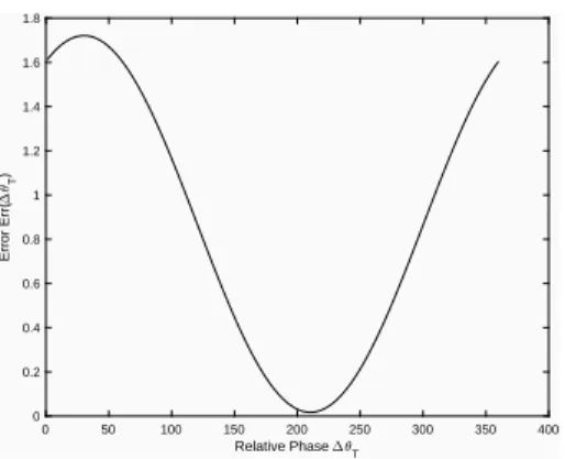
In the next step, we build a error model:
Err(∆ϕT) = X
i
[pi−pT i(∆ϕT)]2 (11)
wherei= 1...4 stands for the 4 phases Alice modulates,pT i(∆ϕT) is the theoretical result of
the detection probability assume the relative phase between Alice’s and Bob’s fiber is ∆ϕT.
These theoretical probabilities are calculated with:
pT i(∆ϕT) = cos2(
∆θi+ ∆ϕT
2 ) (12)
the phase differences are ∆θi ={0, π/2, π, 3π/2}, for i= 1...4.
The final step is to minimize Err(∆ϕT), as this value will be minimized when ∆ϕT is the
same as the practical one. We traversing ∆ϕT from 0 to 360 degree, with 1 degree as a step.
The phase ∆ϕT min that minimizeErr(∆ϕT) is recorded as the estimated phase difference.
In the mean time, we also record the maximal value of Err(∆ϕT), and define a parameter:
rc= min[Err(∆ϕT)]/max[Err(∆ϕT)] (13)
The parameter rc represent whether the pi distribution is close to the theoretical one.
Since the valuercmeasures the ratio between the minimum and the maximum, it approaches 0 when the measured distribution is perfect, while approaches 1 when the four phase reference
pulses have the same counts. We use this parameter as an indicator of the correctness of the estimation result. In the experiment, we keep only the detections that the rc value of the reference pulses is small. As discussed in main test, this is done only with the phase reference pules in Charlie’s measurement station. The security still holds for this operation is uniformly on all detections, whether Alice (Bob) sends Z or X basis.
TABLE I. Measured reference counts and probabilities for a 10µstime span. The estimated phase difference of the fiber is ∆ϕT = 209◦, the phase estimation success probability rc = 0.01. In the table, we also show the theoretical probabilities calculated at ∆ϕT = 209◦.
Relative Phase ∆θ 0 π/2 π 3π/2 Measured Counts 4.15 16.60 22.55 6.25 Measured Probabilities 0.168 0.670 0.910 0.252 Theoretical Probabilities 0.063 0.742 0.937 0.258
Take the values in Tab. I as an example, “Measured Counts” stands for the detections in 10µsfor the four different phases, “Measured Probabilities” are the normalized probabilities calculated with Eq. 10. Note we assume a 40 ns dead time and the “Measured Counts” are recovered with the detection efficiencies and the dead time. Next we optimize the error with Eq. 11 to obtain the estimated phase difference. In our experiment, we calculate the error with ∆ϕT varying from 0 to 360, the result is shown in Fig. 8. From this result, we can read
the most possible phase difference is ∆ϕT = 209◦, the phase estimation success probability
rc= 0.01.
The phase estimation success probability rc is different for different time period with different environment and noise. Take the data measured in 100 km as an example, we calculate the distribution ofrcfor the time period where there are detections, shown in Fig. 9. For each fiber distance, we optimize thercvalues for the maximum final key rate. Normally, the value rc = 0.01 with around 14% data kept is the best choice for our experiment. The value varies with the channel condition.
D. Compensate the relative phase due to the fiber in post-processing
In the theoretical analysis, it always assume the relative phase due to the fiber (∆ϕT)
0 50 100 150 200 250 300 350 400 Relative Phase T 0 0.2 0.4 0.6 0.8 1 1.2 1.4 1.6 1.8 Error Err( T )
FIG. 8. Calculated Error Err(∆ϕT) against the phase difference ∆ϕT.
FIG. 9. Distribution of rc, statistics with 100 km data.
with a fast feedback circuit. In our experiment, however, we can estimate the relative phase as in the above sections. In the following, we show the compensation procedure with the relative phase:
In SNS-TF-QKD, we need to set a reasonable phase slice criterion for post selection of
X-basis events so as to make a reasonable estimation of error rate in X-basis. Here in our experiment, the channel (Charlie) does not take the active compensation and hence we use the following criterion for the post selection:
1− |cos(θA−θB+ ∆ϕT)|<Λ (14)
with the estimated value of relative phase ∆ϕT. The original equation requires the phase
difference between Alice and Bob is smaller than Ds orDs+π. With the revised equation,
the phase difference after the fiber|θA−θB+∆ϕT|falls in the range, i.e.,|θA−θB+∆ϕT|< Ds
or|θA−θB+ ∆ϕT|< Ds+π, with high probability. Thus, the error due to the interference
In a short conclusion, we use phase reference pulse to estimate the phase difference between Alice’s and Bob’s fiber. The method requires an intensity of less than 50 total detections in 10 µs time span. Thus, the required intensity of the laser source is not too strong even the communication distance is several hundred kilometers. A relative weak reference pulse also reduces noises, which is a severe problem to long distance communication. Also, the method does not require a fast feedback circuit, decreasing the difficulty of the system.
III. DETAILED EXPERIMENTAL PARAMETERS
We summarize the parameter we used in our experiment in Tab. II.
The fiber distance between Alice (Bob) and Charlie are the same, “fiber length” in the table is the total fiber length, µ1,µ2 and µz are the intensities for the decoy states and the
signal state. Note that the intensity of the weak decoy state µ1 is fixed to a mean photon number of 0.05. We do not use the optimized value, which is smaller, mainly due to the performance limitation of the intensity modulators. Stable intensity modulation are required in the decoy state modulation. However, the modulator is sensitive and vary during time if the extinction ratio is too high. Thus, we fix the lowest intensity to ensure the decoy intensities are stable.
µref denotes the intensity of the phase reference pulse, in the same pulse width as the
signal pulse (2 ns). This intensity only calculates the time the phase reference pulse is not modulated to vacuum, the “reference width” indicate the time interval Alice (Bob) send reference pulse in each 300 ns time span. We did not send the pulses during all the 300 ns time span for a few reasons: with a appropriate ratio, the intensity of the phase reference pulse is not too strong or too weak, thus easier for modulation; the response frequency of the modulators are limited, we need to modulate with appropriate frequencies.
In total, Ntotal signal pulses are sent for different fiber distances. The ratio of sending X
(Z) basis is pX (pZ). In X basis, the ratio of sending the decoy states vacuum, µ1 and µ2 are p0, p1 and p2. In Z basis, the ratio of “sending” and “not-sending” pulses are pz1 and
pz0. We use the fixed ratio because of limited amplifier and modulator response frequency. The cutoff frequencies of our amplifiers and modulators are between 10 MHz and 10 GHz. Thus, the response will become nonlinear if no signal are produced for a long time, which
may happen when the ratio of sending Z basis is high. We avoid this scenario by fix the ratio sending X basis. With better electronic components, the optimized parameters can be used in the experiment to further enhance the final key rate.
Finally, based on the above parameters, we calculate the output intensity at Alice’s (Bob’s) output. We also estimate the detection counts, considering all the optics efficiencies and the detection efficiencies. However, when the detection counts are large, the detector dead time further decrease the detection efficiencies. The peak intensity of the phase refer-ence pulses is around 2 ∼ 5 photons per 100 ns, which is high for the detector. Thus, the actual detection counts are smaller than the theoretical expectation. We need to note that this effect does not affect the detection efficiency of the signal pulses.
TABLE II. Experimental parameters for different fiber lengths. Fiber Length 0 km 50 km 100 km 150 km µ1 0.050 0.050 0.050 0.050 µ2 0.159 0.160 0.177 0.197 µz 0.557 0.480 0.452 0.433 µref 0.156 0.371 1.173 0.824 pX 0.300 0.300 0.300 0.300 pZ 0.700 0.700 0.700 0.700 p0 0.250 0.250 0.250 0.250 p1 0.500 0.500 0.500 0.500 p2 0.250 0.250 0.250 0.250 pz0 0.978 0.978 0.978 0.978 pz1 0.022 0.022 0.022 0.022 Reference Width (ns) 100 100 100 300 Output Intensity (pW) 0.98 1.97 6.07 19.05 Target Detections (MHz) 4.36 3.11 3.03 3.01
IV. DETAILED EXPERIMENTAL RESULT
We characterize our experimental system and perform the experimental test with different fiber length. The result is summarized in Tab. III, Tab. IV, and Tab. V.
In Tab. III, we measure the transmittance of the fiber, the fiber optical elements, and the efficiencies of the SNSPDs. For the optical elements, we measure the optical transmittance including the polarization controller(PC-A/PC-B), the polarization beam splitter(PBS-A/PBS-B), and the beam splitter. As there are two inputs (A/B) and two outputs (ch1/ch2), the transmittance is noted with the inputs and the outputs. The SNSPD efficiencies is mea-sured with including the efficiency of the polarization controller.
TABLE III. Experimental parameters for different fiber lengths. Fiber Length 0 km 50 km 100 km 150 km ηF iberA 1 0.315 0.112 0.038 ηF iberB 1 0.316 0.120 0.033 PC-A 94.2% PC-B 92.8% PBS-A 91.1% PBS-B 86.5% BS-A-ch1 36.9% BS-A-ch2 38.6% BS-B-ch1 39.1% BS-B-ch2 41.4 % SNSPD-ch1 75.31% SNSPD-ch2 76.56%
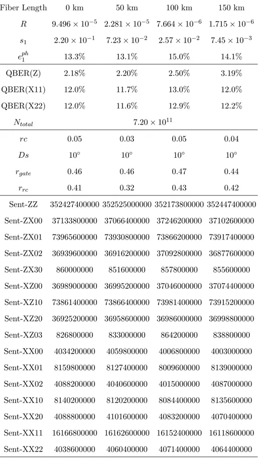
The experimental result are summarized in Tab. IV and Tab. V. For each fiber distance, we write here the final key rate (R) with the best parameters including the accepted phase difference (Ds, in degree), and the parameter describing the phase estimation success prob-ability (rc). The proportion of data accepted with smallerrcis denoted with the parameter
rrc. In the experimental implementation, a digital window is applied to select the signal in
data falling in this window is measured with the parameter rgate. Note all the detections
are filtered by the digital window and by the estimation success probability (rc) in Charlie, before announcing the detections.
In this table, we summarize the raw data used for calculation. The total number of signal pulses is denoted as Ntotal , The error rate in Z basis and in X basis are QBER(Z)
and QBER(X11)/QBER(X22), where “11” and “22” are the decoy states used. In the next lines, the number of pulses Alice and Bob sent in different decoy states are listed. We label these numbers with “Sent-ABCD”, where “A” (“B”) is “X” or “Z” standing for the basis Alice (Bob) uses; “C” (“D”) is “0”, “1”, “2” or “3”, indicating the intensity Alice (Bob) uses is “vacuum”, “µ1”, “µ2” or “µz”. The total number of pulses Alice and Bob sent is labeled
with “Sent-AB”. Similar as the number of sent pulses, We label the number of detections as “Detected-ABCD”. The numbers of detections falling in the accepted difference range (Ds) are also summarized in the table, labeled with “Detected-ABCD-Ds-Ch”, where “Ds” means only the data within the accepted Ds range are counted, “Ch” indicate in which detection channel the events are detected. The numbers of correct detections are labeled with “Correct-ABCD-Ds-Ch”, with which numbers we can calculate the error rate in X basis. The optimized accept range is listed on the top lines of this table.
For different phase difference range (Ds) and for the accepted phase estimation success probability (rc), the QBERs in X basis and the detection counts are different. In the above Tab. IV and Tab. V, we optimize these value to obtain a maximum final key rate. Take the data in 150 km for example, the QBERs in X basis when Alice and Bob send decoy states
µ1 and µ2 are listed in Tab. VI and Tab. VII, the detections in Tab. VIII and Tab. IX, respectively. The secure key rates with different parameters are calculated and summarized in Tab. X. Note that in key rate calculation, we search different ranges for the optimized key rate. In this data set, the optimized key rate is obtained with Ds/2=10◦ and rc=0.04, where Ds/2 is half of the phase difference range.
[1] C. BENNETT, inProceedings of the IEEE International Conference on Computers, Systems, and Signal Processing (1984) pp. 175–179.
[3] M. Duˇsek, N. L¨utkenhaus, and M. Hendrych, Progress in Optics 49, 381 (2006).
[4] V. Scarani, H. Bechmann-Pasquinucci, N. J. Cerf, M. Duˇsek, N. L¨utkenhaus, and M. Peev, Reviews of modern physics 81, 1301 (2009).
[5] S.-K. Liao, W.-Q. Cai, W.-Y. Liu, L. Zhang, Y. Li, J.-G. Ren, J. Yin, Q. Shen, Y. Cao, Z.-P. Li, et al., Nature549, 43 (2017).
[6] S.-K. Liao, W.-Q. Cai, J. Handsteiner, B. Liu, J. Yin, L. Zhang, D. Rauch, M. Fink, J.-G. Ren, W.-Y. Liu, et al., Physical review letters 120, 030501 (2018).
[7] L. Lydersen, C. Wiechers, C. Wittmann, D. Elser, J. Skaar, and V. Makarov, Nature photonics 4, 686 (2010).
[8] W.-Y. Hwang, Physical Review Letters91, 057901 (2003). [9] X.-B. Wang, Physical review letters 94, 230503 (2005).
[10] H.-K. Lo, X. Ma, and K. Chen, Physical review letters94, 230504 (2005). [11] M. Lucamarini, Z. Yuan, J. Dynes, and A. Shields, Nature 557, 400 (2018).
[12] Q. Zhang, F. Xu, Y.-A. Chen, C.-Z. Peng, and J.-W. Pan, Optics express26, 24260 (2018). [13] Y.-L. Tang, H.-L. Yin, S.-J. Chen, Y. Liu, W.-J. Zhang, X. Jiang, L. Zhang, J. Wang, L.-X. You, J.-Y. Guan, D.-X. Yang, Z. Wang, H. Liang, Z. Zhang, N. Zhou, X. Ma, T.-Y. Chen, Q. Zhang, and J.-W. Pan, Phys. Rev. Lett. 113, 190501 (2014).
[14] S. L. Braunstein and S. Pirandola, Physical review letters108, 130502 (2012). [15] H.-K. Lo, M. Curty, and B. Qi, Physical review letters 108, 130503 (2012). [16] Y.-H. Zhou, Z.-W. Yu, and X.-B. Wang, Physical Review A 93, 042324 (2016).
[17] H.-L. Yin, T.-Y. Chen, Z.-W. Yu, H. Liu, L.-X. You, Y.-H. Zhou, S.-J. Chen, Y. Mao, M.-Q. Huang, W.-J. Zhang, et al., Physical review letters 117, 190501 (2016).
[18] A. Boaron, G. Boso, D. Rusca, C. Vulliez, C. Autebert, M. Caloz, M. Perrenoud, G. Gras, F. Bussi`eres, M.-J. Li, et al., Physical review letters 121, 190502 (2018).
[19] M. Takeoka, S. Guha, and M. M. Wilde, Nature communications5, 5235 (2014).
[20] S. Pirandola, R. Laurenza, C. Ottaviani, and L. Banchi, Nature communications 8, 15043 (2017).
[21] X.-B. Wang, Z.-W. Yu, and X.-L. Hu, Physical Review A 98, 062323 (2018).
[22] Z.-W. Y. Yu, X.-L. Hu, C. Jiang, H. Xu, and X.-B. Wang, arXiv preprint arXiv:1807.09891 (2018).
Physics B 31, 97 (1983).
[24] R. V. Pound, Review of Scientific Instruments17, 490 (1946).
[25] S. Miki, M. Yabuno, T. Yamashita, and H. Terai, Optics Express25, 6796 (2017).
[26] A. J. Kerman, E. A. Dauler, W. E. Keicher, J. K. Yang, K. K. Berggren, G. Gol’Tsman, and B. Voronov, Applied physics letters 88, 111116 (2006).
[27] D.-K. Liu, S.-J. Chen, L.-X. You, Y.-L. Wang, S. Miki, Z. Wang, X.-M. Xie, and M.-H. Jiang, Applied Physics Express 5, 125202 (2012).
[28] S. Droste, F. Ozimek, T. Udem, K. Predehl, T. H¨ansch, H. Schnatz, G. Grosche, and R. Holzwarth, Physical review letters 111, 110801 (2013).
TABLE IV. Experimental results for different fiber lengths. Fiber Length 0 km 50 km 100 km 150 km R 9.496×10⁻⁵ 2.281×10⁻⁵ 7.664×10⁻⁶ 1.715×10⁻⁶ s1 2.20×10⁻¹ 7.23×10⁻² 2.57×10⁻² 7.45×10⁻³ eph1 13.3% 13.1% 15.0% 14.1% QBER(Z) 2.18% 2.20% 2.50% 3.19% QBER(X11) 12.0% 11.7% 13.0% 12.0% QBER(X22) 12.0% 11.6% 12.9% 12.2% Ntotal 7.20×10¹¹ rc 0.05 0.03 0.05 0.04 Ds 10◦ 10◦ 10◦ 10◦ rgate 0.46 0.46 0.47 0.44 rrc 0.41 0.32 0.43 0.42 Sent-ZZ 352427400000 352525000000 352173800000 352447400000 Sent-ZX00 37133800000 37066400000 37246200000 37102600000 Sent-ZX01 73965600000 73930800000 73866200000 73917400000 Sent-ZX02 36939600000 36916200000 37092800000 36877600000 Sent-ZX30 860000000 851600000 857800000 855600000 Sent-XZ00 36989000000 36995200000 37046000000 37074400000 Sent-XZ10 73861400000 73866400000 73981400000 73915200000 Sent-XZ20 36925200000 36958600000 36986000000 36998800000 Sent-XZ03 826800000 833000000 864200000 838800000 Sent-XX00 4034200000 4059800000 4006800000 4003000000 Sent-XX01 8159800000 8127400000 8009600000 8139000000 Sent-XX02 4088200000 4040600000 4015000000 4087000000 Sent-XX10 8140200000 8120200000 8084400000 8135600000 Sent-XX20 4088800000 4101600000 4083200000 4070400000 Sent-XX11 16166800000 16162600000 16152400000 16118600000 Sent-XX22 4038600000 4060400000 4071400000 4064400000
TABLE V. Experimental results for different fiber lengths. Fiber Length 0 km 50 km 100 km 150 km Detected-ZX00 33179 18044 23574 18883 Detected-ZX01 253374727 74427515 31550408 9356926 Detected-ZX02 402438421 114186348 55219631 18763685 Detected-ZX30 30774678 7654434 3160510 983736 Detected-XZ00 33316 18000 23153 18781 Detected-XZ10 243332100 70866220 28911062 9001415 Detected-XZ20 383172746 110124270 52860174 18303719 Detected-XZ03 30611835 7574806 3185989 923116 Detected-XX00 3563 1910 2529 2047 Detected-XX01 27973801 8192443 3419006 1028370 Detected-XX02 44545111 12516886 5981633 2084672 Detected-XX10 26835876 7786310 3154146 990573 Detected-XX20 42404015 12207818 5845716 2004057 Detected-XX11 107700658 31698647 13173657 3992955 Detected-XX22 83470873 24461170 11799518 4042977 Detected-XX11-Ds-Ch1 6030273 1782747 738886 222421 Detected-XX11-Ds-Ch2 6476445 1909673 797997 241777 Correct-XX11-Ds-Ch1 5302155 1574536 642684 195446 Correct-XX11-Ds-Ch2 5702371 1687713 694483 212980
TABLE VI. QBER in X basis in decoy state µ1 with 150 km fiber.
RC|Ds/2 deg=1◦ deg=2◦ deg=4◦ deg=6◦ deg=8◦ deg=10◦ deg=12◦ deg=15◦ rc=0.01 9.60% 9.70% 9.70% 9.80% 9.90% 9.90% 10.0% 10.2% rc=0.02 10.6% 10.6% 10.6% 10.6% 10.7% 10.8% 10.8 % 11.0% rc=0.04 11.9% 12.0% 11.9% 11.9% 12.0% 12.0% 12.1 % 12.2% rc=0.05 12.5% 12.6% 12.5% 12.5% 12.5% 12.6% 12.6 % 12.8% rc=0.10 14.9% 15.0% 14.8% 14.8% 14.8% 14.8% 14.9 % 15.0%
TABLE VII. QBER in X basis in decoy state µ2 with 150 km fiber.
RC|Ds/2 deg=1◦ deg=2◦ deg=4◦ deg=6◦ deg=8◦ deg=10◦ deg=12◦ deg=15◦ rc=0.01 9.60% 9.60% 9.80% 9.90% 10.0% 10.0% 10.2% 10.4% rc=0.02 10.5% 10.5% 10.5% 10.6% 10.7% 10.8% 10.9% 11.1% rc=0.04 12.0% 12.0% 12.0% 12.1% 12.2% 12.2% 12.2% 12.4% rc=0.05 12.6% 12.6% 12.6% 12.6% 12.7% 12.7% 12.8% 12.9% rc=0.10 14.8% 14.9% 14.9% 14.9% 15.0% 14.9% 15.0% 15.1%
TABLE VIII. Detections in X basis in decoy state µ1 with 150 km fiber.
RC|Ds/2 deg=1◦ deg=2◦ deg=4◦ deg=6◦ deg=8◦ deg=10◦ deg=12◦ deg=15◦ rc=0.01 25920 43810 77901 112095 146611 181930 216085 269071 rc=0.02 42331 71760 129987 188283 248574 309691 370416 462085 rc=0.04 63617 107070 193671 282255 372405 464198 555951 693152 rc=0.05 70817 119687 216583 314920 415225 517508 619325 772151 rc=0.10 94310 159293 287220 417054 549170 682478 815517 1015767
TABLE IX. Detections in X basis in decoy stateµ2 with 150 km fiber.
RC|Ds/2 deg=1◦ deg=2◦ deg=4◦ deg=6◦ deg=8◦ deg=10◦ deg=12◦ deg=15◦ rc=0.01 25623 43760 77889 112020 146619 181508 215655 268197 rc=0.02 41921 71575 129710 188161 248720 309052 369819 460779 rc=0.04 63038 106851 193420 281872 372448 463651 555692 692316 rc=0.05 70180 119398 216221 314377 415230 516792 618938 771397 rc=0.10 93939 159293 287262 417313 550154 682961 816726 1016446
TABLE X. Key Rate for different parameters with 150 km fiber.
RC|Ds/2 deg=1◦ deg=2◦ deg=4◦ deg=6◦ deg=8◦ deg=10◦ deg=12◦ deg=15◦ rc=0.01 0 4.71×10⁻⁷ 8.29×10⁻⁷ 9.51×10⁻⁷ 9.97×10⁻⁷ 1.02×10⁻⁶ 1.03×10⁻⁶ 1.01×10⁻⁶ rc=0.02 0 7.62×10⁻⁷ 1.28×10⁻⁶ 1.47×10⁻⁶ 1.51×10⁻⁶ 1.52×10⁻⁶ 1.52×10⁻⁶ 1.49×10⁻⁶ rc=0.04 0 5.84×10⁻⁷ 1.39×10⁻⁶ 1.61×10⁻⁶ 1.70×10⁻⁶ 1.71×10⁻⁶ 1.71×10⁻⁶ 1.69×10⁻⁶ rc=0.05 0 3.10×10⁻⁷ 1.23×10⁻⁶ 1.49×10⁻⁶ 1.60×10⁻⁶ 1.61×10⁻⁶ 1.62×10⁻⁶ 1.58×10⁻⁶ rc=0.10 0 0 1.17×10⁻⁸ 4.05×10⁻⁷ 5.71×10⁻⁷ 6.40×10⁻⁷ 6.67×10⁻⁷ 6.44×10⁻⁷