METHODOLOGY ARTICLE
Supplementary to parameter estimation of
dynamic biological network models using
integrated fluxes
Yang Liu and Rudiyanto Gunawan
**Correspondence: [email protected] Institute for Chemical and Bioengineering, ETH Zurich, Vladimir-Perlog-Weg 1, 8093 Zurich, Switzerland
Full list of author information is available at the end of the article
min
𝐗
𝑈0,𝐩
𝐼Φ 𝐗
𝑈0
, 𝐩
𝐼
, 𝐗
𝑀
s. t.
𝐗
𝑈≥ 0
𝐩
𝐼∈ 𝐋
𝐼, 𝐔
𝐼𝛈 𝑡
𝑘≥ 0
2. Calculate independent IFs 𝛈𝐼,𝑘𝐗𝑀, 𝐩𝐼 = ⋮ 𝑣𝑗𝐗𝑀, 𝐩𝐼𝑑𝑡 𝑡𝑘 0 ⋮ 𝑛−𝑚 ×1
4. Estimate the parameters associated with dependent IFs
𝐩𝐷∗= argmin 𝐩𝐷∈ 𝐋𝐷,𝐔𝐷
Φ𝑖𝑛𝐩𝐷, 𝛈𝐷, 𝐗𝑀
3. Solve for dependent IFs
𝐗𝑀𝑡𝑘 − 𝐗𝑀0 = 𝐒𝐼 𝐒𝐷 𝛈𝐼,𝑘𝛈𝐗𝑀, 𝐩𝐼 𝐷𝑡𝑘
𝛈𝐷𝑡𝑘 = 𝐒𝐷−1𝐗𝑀𝑡𝑘 − 𝐗𝑀0 − 𝐒𝐼𝛈𝐼,𝑘𝐗𝑀, 𝐩𝐼
1. Simulate unmeasured 𝐗𝑈 𝐗 𝑈= 𝐒𝑈𝐯 𝐗𝑀, 𝐗𝑈, 𝐩𝐼; 𝐗𝑈0 = 𝐗𝑈0
5. Compute objective function Φ 𝐩𝐼, 𝐗𝑀
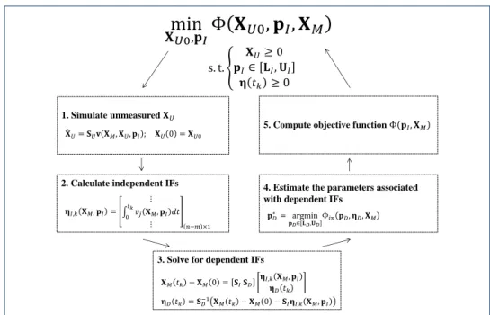
Figure S1 Flowchart of integrated flux parameter estimation (IFPE) with unmeasured concentrations. These unmeasured species are denoted byXU. All reactions and parameters appearing inX˙Uare selected as independent fluxes and parameters. The first step in calculating Φinvolves simulating unmeasured concentrationXUby solving ODEsX˙U=SUv(XM,XU,pI), where the measured concentrationsXM are treated as external input variables. The subsequent steps are the same as in the IFPE methods without unmeasured concentrations. An example using the branched pathway model is shown in Figure S3.
1 Modified Simpson’s rule
We performed the integration of flux function
η
(
X
,
p
) =
R
t0
v
(
X
,
p
)
dt
using the
following modified Simpson’s quadrature rule:
Z
t2 t1f
(
t
)
dt
≈
t
2−
t
16
2 + 3
β
1 +
β
f
(
t
1) +
1 + 3
β
β
f
(
t
2)
−
1
β
(1 +
β
)
f
(
t
3)
,
(1)
where
β
= (
t
3−
t
2)
/
(
t
2−
t
1). The quadrature function above was derived from the
ordinary Simpson’s rule, by calculating the shaded area of the quadratic
polyno-mial determined by three points (
t
1, f
(
t
1)), (
t
2, f
(
t
2)), and (
t
3, f
(
t
3)) as illustrated
tributed time points, the quadrature function above reduces to (by setting
β
= 1):
Z
t2t1
f
(
t
)
dt
≈
dt
12
[5
f
(
t
1) + 8
f
(
t
2)
−
f
(
t
3)]
.
(2)
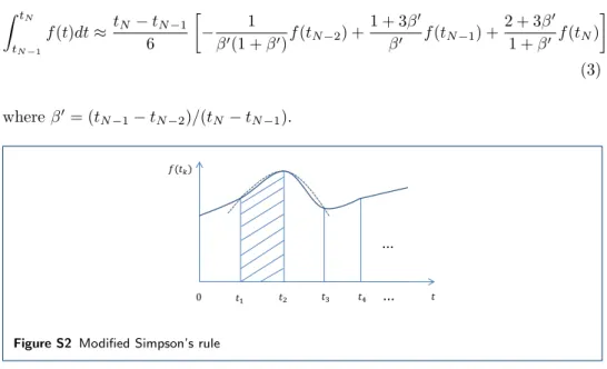
To calculate the integral between last two time points, the area between
t
N−1and
t
Nunder the curve of the quadratic polynomial is
Z
tN tN−1f
(
t
)
dt
≈
t
N−
t
N−16
−
1
β
0(1 +
β
0)
f
(
t
N−2) +
1 + 3
β
0β
0f
(
t
N−1) +
2 + 3
β
01 +
β
0f
(
t
N)
,
(3)
where
β
0= (
t
N−1−
t
N−2)
/
(
t
N−
t
N−1).
͘͘͘
͘͘͘
Figure S2 Modified Simpson’s rule
2 Supplementary information for the branched pathway case
study
We generated the
in silico
data by simulating the ODE model in Eqs. (11) and
(12) using the parameter values:
a
1= 12,
g
13= 0
.
8,
a
2= 8,
g
21= 0
.
5,
a
3= 3,
g
32= 0
.
75,
a
4= 5,
g
43= 0
.
5,
g
44= 0
.
2,
a
5= 2,
g
51= 0
.
5,
a
6= 6,
g
64= 0
.
8, and
the initial conditions:
X
1(0)
X
2(0)
X
3(0)
X
4(0)
=
1
.
4
2
.
7
1
.
2
0
.
4
.
0 1 2 3 4 5 0 0.5 1 1.5 X 1 0 1 2 3 4 5 1.5 2 2.5 3 3.5 X 2 0 1 2 3 4 5 0 1 2 3 X 3 0 1 2 3 4 5 0.1 0.2 0.3 0.4 0.5 X 4 time concentration
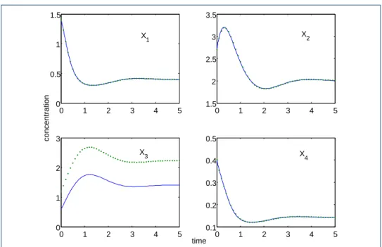
Figure S3 Parameter estimation of the branched pathway model using noise-free data without the concentration measurements ofX3 using the IFPE without ODE integration. The solid lines and
dots represent the model prediction and the true concentrations, respectively.
0 1 2 3 4 5 0 2 4 (s, o) = (3, 3) 0 1 2 3 4 5 0 2 4 (s, o) = (5, 3) 0 1 2 3 4 5 0 2 4 (s, o) = (3, 5) 0 1 2 3 4 5 0 2 4 (s, o) = (3, 3) 0 1 2 3 4 5 0 2 4 (s, o) = (5, 3) 0 1 2 3 4 5 0 2 4 (s, o) = (3, 5) time concentration
Figure S4 Smoothened time-series concentration data using different piecewise spline-fitting parameters for the branched pathway case study. The parameterssandoindicate the number of pieces and the degree of polynomials, respectively. The plots in first row show noise-free data, while the plots in second row show one noisy dataset (out of five technical replicates) with 10% coefficient of variation of Gaussian noise.
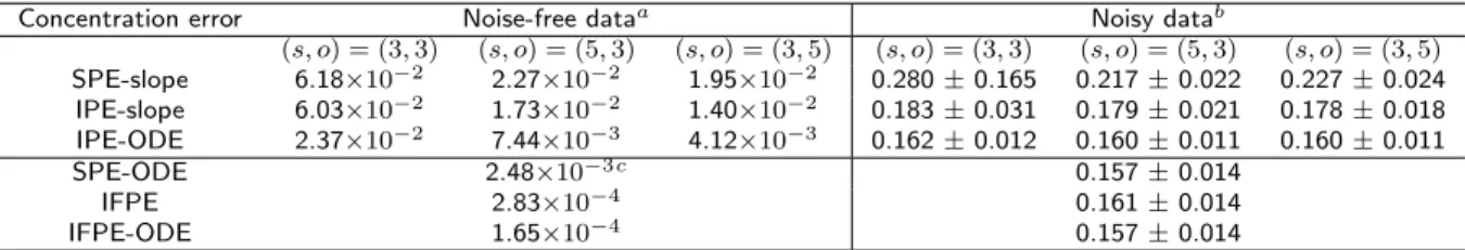
Concentration error Noise-free data Noisy data (s, o) = (3,3) (s, o) = (5,3) (s, o) = (3,5) (s, o) = (3,3) (s, o) = (5,3) (s, o) = (3,5) SPE-slope 6.18×10⁻² 2.27×10⁻² 1.95×10⁻² 0.280±0.165 0.217±0.022 0.227±0.024 IPE-slope 6.03×10⁻² 1.73×10⁻² 1.40×10⁻² 0.183±0.031 0.179±0.021 0.178±0.018 IPE-ODE 2.37×10⁻² 7.44×10⁻³ 4.12×10⁻³ 0.162±0.012 0.160±0.011 0.160±0.011 SPE-ODE 2.48×10⁻³c 0.157±0.014 IFPE 2.83×10⁻⁴ 0.161±0.014 IFPE-ODE 1.65×10⁻⁴ 0.157±0.014
a. For noise-free data, five independent runs were carried out. The concentration error is reported for the run with the lowest objective function value.
b. For noisy data, the reported values are the mean±standard deviation of five technical replicates of the data.
c. Only three out of five repeated runs finished within 24 hours. The concentration error is reported for the run with the lowest objective function value among the three successful runs.
Table S2 Comparison of median parameter errors for the branched pathway case study with different partitioning of independent and dependent flux set.
Median parameter errora(%) Noise-free datab Noisy datac
Independent fluxes IFPE IFPE-ODE IFPE IFPE-ODE
{V1, V6}d 0.276 0.746 66.9±32.5 70.0±31.6 {V1, V5} 0.293 0.734 64.0±33.0 50.6±26.9 {V2, V6} 0.270 1.00 68.6±32.2 70.7±27.7 {V1, V3} 0.262 0.755 59.1±26.4 60.6±15.0 {V2, V5} 0.281 0.975 66.1±27.9 66.8±33.8 {V1, V4} 0.238 0.839 60.3±29.6 68.5±20.9
a. The median is taken over 13 parameters in the branched pathway model.
b. For noise-free data, five independent runs were carried out. The median parameter error corresponds to the run with the lowest objective function value.
c. For noisy data, the reported values are the mean±standard deviation of five technical replicates of the data.
d. Independent flux combination used in the main text.
Table S3 Comparison of CPU times for the branched pathway case study with different partitioning of independent and dependent flux set.
CPU timea(sec) Noise-free datab Noisy datac
Independent fluxes IFPE IFPE-ODE IFPE IFPE-ODE
{V1, V6}d 1263 2154 655.9±198.5 1023±315 {V1, V5} 1806.8 2912.3 677.4±205.0 956.6±231.0 {V2, V6} 1995.7 1775.4 1190.1±332.6 1809.9±589.4 {V1, V3} 1152.9 2399.7 562.6±334.2 1529.9±656.5 {V2, V5} 2961.8 3659.2 1285.9±141.1 2055.4±392.8 {V1, V4} 1527.0 3267.9 1067.8±890.5 1241.8±299.0
a. The CPU times were recorded using a workstation with Intel Xeon processor 3.33GHz with 18GB RAM.
b. For noise-free data, five independent runs were carried out. The CPU time is reported for the run with the lowest objective function value.
c. For noisy data, the reported values are the mean±standard deviation of five technical replicates of the data.
d. Independent flux combination used in the main text.
Table S4 Comparison of the number of eSS iterations for the branched pathway case study with different partitioning of independent and dependent flux set.
eSS iterations Noise-free dataa Noisy datab Independent fluxes IFPE IFPE-ODE IFPE IFPE-ODE
{V1, V6}c 112 156 67.0±13.1 70.2±11.8 {V1, V5} 158 201 64.2±5.9 66.8±2.9 {V2, V6} 147 86 92.0±35.8 96.8±41.4 {V1, V3} 169 241 113.0±61.0 151.6±69.2 {V2, V5} 194 160 63.4±2.6 80.6±31.6 {V1, V4} 162 252 154.0±75.1 78.6±15.2
a. For noise-free data, five independent runs were carried out. The number of eSS iterations corresponds to the run with the lowest objective function value.
b. For noisy data, the reported values are the mean±standard deviation of five technical replicates of the data.
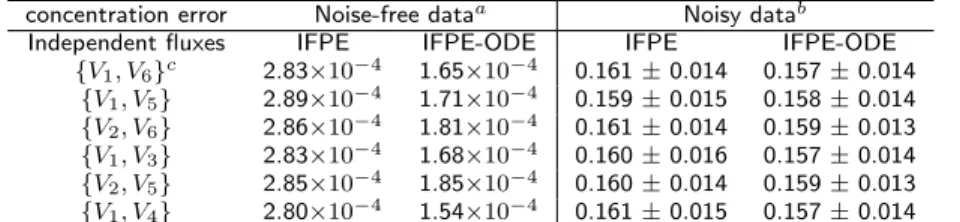
Table S5 Comparison of concentration errorΦfor the branched pathway case study with different partitioning of independent and dependent flux set.
concentration error Noise-free dataa Noisy datab
Independent fluxes IFPE IFPE-ODE IFPE IFPE-ODE
{V1, V6}c 2.83×10⁻⁴ 1.65×10⁻⁴ 0.161±0.014 0.157±0.014 {V1, V5} 2.89×10⁻⁴ 1.71×10⁻⁴ 0.159±0.015 0.158±0.014 {V2, V6} 2.86×10⁻⁴ 1.81×10⁻⁴ 0.161±0.014 0.159±0.013 {V1, V3} 2.83×10⁻⁴ 1.68×10⁻⁴ 0.160±0.016 0.157±0.014 {V2, V5} 2.85×10⁻⁴ 1.85×10⁻⁴ 0.160±0.014 0.159±0.013 {V1, V4} 2.80×10⁻⁴ 1.54×10⁻⁴ 0.161±0.015 0.157±0.014
a. For noise-free data, five independent runs were carried out. The concentration error is reported for the run with the lowest objective function value.
b. For noisy data, the reported values are the mean±standard deviation of five technical replicates of the data.