Paper 270-2009
Maximizing the Performance of Your SAS
®Solution: Case Studies in Web
Application Server Tuning for n-tier SAS Applications
Nicholas Eayrs, Tanya Kalich, Graham Lester, and Stuart Rogers, SAS Institute Inc.
ABSTRACT
Are there changes you could make in your Java Web Application Server that would make your SAS solution more responsive, more robust, or able to handle a larger client load? This presentation highlights the settings that are most likely to affect the smooth functioning of your SAS solution and explains the concepts behind those settings. Case studies from SAS Technical Support are used to illustrate a broad range of potential pitfalls, narrowly avoided disasters, and wild successes. The presentation also delves into the troubleshooting techniques you need in order to identify problems in Java Web Application Server tuning and to pinpoint the best solutions.
INTRODUCTION
The SAS®9 architecture for the majority of products and solutions includes a middle tier. This middle tier runs a Java Web Application Server to provide both dynamic Web clients and messaging. For SAS®9, the supported Java Web Application servers are Apache Tomcat, BEA WebLogic Server, and IBM WebSphere Application Server. This paper examines the options that are available for all three Java Web Application Servers and clearly defines the points at which the servers behave differently. This paper follows a basic flow, which starts with an examination of the methods that are required to make the current single Java Web Application Server more responsive and more robust. The examination includes the following:
• reviewing WebLogic and WebSphere timeout issues
• reviewing definitions of memory allocation within the Java Web Application Server • investigating the process of memory management
• investigating the options that are available for optimizing the use of multi-threading capabilities.
After examining the single-server instance, this paper investigates methods for enabling the Java Web Application Server to handle a larger client load. This part of the investigation focuses on scaling the Java Web Application Server both vertically on a single machine and horizontally across a number of machines. Throughout the investigation, the theory of what can be tuned or changed is presented, followed by specific case studies that highlight the benefits and potential pitfalls of each area.
This paper focuses on topics that are relevant for administrators, architects, and implementers of SAS solutions. Despite the complexity of the information and techniques presented in this paper, you should always start with the simplest solutions. As a case in point, perhaps the way you use your SAS solution is the underlying problem rather than the technology. For example, a trillion-row report in SAS® Web Report Studio never runs instantaneously. In fact, such a large report might cause the system to time out, as shown in Figure 1. You need to consider whether it is really necessary to run such reports in real time. Can you run the reports in batch overnight and then view the static results later? Is it possible to split the user community and have people access different middle tiers?
Figure 1. Extremely large reports can cause timeout issues
Finally, if you decide to upgrade your Java Web Application Server, see "SAS® Third-Party Software Requirements - Baseline and Higher Support" for the latest baseline-support statement.
OVERVIEW OF SUPPORTED JAVA WEB APPLICATION SERVERS
This section discusses key differences in the three Java Web Application Servers that are supported in SAS®9 software: Apache Tomcat, BEA WebLogic Server, and IBM WebSphere Application Server.
The following table summarizes the key features of each of the supported Java Web Application Servers: Apache Tomcat BEA WebLogic Server IBM WebSphere Application Server Java 2 Platform, Enterprise Edition (J2EE)
specification
NONE 1.3 1.4
Java 2 Standard Edition (J2SE) specification
J2SE 1.4.2 J2SE 1.4.2 J2SE 5
Servlet 2.3 2.3 2.4
JSP 1.2 1.2 2.0
Administration User Interface O* S* S*
Cluster support O* S* S*
Licensing Terms Open Source Proprietary Proprietary Table 1. Comparison of key features for Java Web Application Servers
* In this table:
• O specifies optional functionality that is provided via third-party implementations. • S specifies standard functionality.
This table illustrates the highest supported revisions and associated capabilities as dictated by SAS®9 third-party software requirements. For further details, see “Third-Party Software for SAS® 9.1.3 Foundation with Service Pack 4.” The next sections describe the key features of each Java Web Application Server in more detail.
APACHE TOMCAT
Apache Tomcat is an open-source implementation based on the Java Servlet and JavaServer Pages (JSP)
technologies; it is the product of collaboration by developers from around the world operating in a non-profit capacity. The Java Servlet specification is a Java Application Programmer Interface (API) that enables developers to create dynamic content for deployment on a Java Web Application Server. This content is typically composed of many JSP files that are compiled into Java Servlets by a JSP compiler. The Java Web Application Server has a component called the Web Container that is responsible for the rendering of servlets.
As of this writing, the current Apache Tomcat version supported by SAS®9 is not Java 2 Platform, Enterprise Edition (J2EE) compliant. It also does not have Enterprise JavaBeans (EJB) capabilities, which limits supported SAS software deployment options (typically the SAS Enterprise Intelligence platform only). Always be sure to consult your specific solution’s system requirements, your SAS Installation Representative, or SAS Technical Support before you implement or procure a Java Web Application Server.
J2EE is a specification developed by the Java Community Process (JCP), a formalized process that defines future releases and functionality of the Java Platform. JCP uses formal request documents (Java Specification Requests, or JSRs) that describe the proposed specification.
The following JSRs are important because SAS solutions are built on each of these JSRs and, as such, the solutions support these specifications:
• JSR58—defines the J2EE 1.3 specification, available at jcp.org/en/jsr/detail?id=58. • JSR151—defines the J2EE.14 specification, available at jcp.org/en/jsr/detail?id=151.
• JSR244—defines the Java Platform, Enterprise Edition (Java EE) 5 specification, available at
jcp.org/en/jsr/detail?id=244.
• JSR220—defines the EJB 3.0 specification, available at jcp.org/en/jsr/detail?id=220. The EJB specification is also a Java API that enables developers to create enterprise class applications that use a true server-side model and focus on manageability, flexibility, and scalability. EJB 3.0 is the latest version.
Apache Tomcat for SAS®9 software supports the following specifications: SAS®9 • Java 2 Standard Edition (J2SE) specification 1.4.2
• Java Servlet 2.3 • JSP 1.2
By default, Tomcat is administered via manual modification of configuration files. You can enhance the administration by implementing third- party administration tools and associated user interfaces.
Clustering can also be achieved via various request-distribution models such as the following: • Domain Name System (DNS)
• Transmission Control Protocol (TCP) Connection Network Address Translation (NAT) • Hypertext Transfer Protocol (HTTP) Redirect Service
• Web Server Connector to Tomcat
BEA WEBLOGIC SERVER
BEA WebLogic Server is a proprietary Java 2 Platform, Enterprise Edition (J2EE) application server that fully supports all SAS software deployments.
BEA WebLogic Server for SAS®9 supports the following specifications: • J2SE specification 1.4.2
• Java Servlet 2.3 • JSP 1.2
An administration interface and cluster support are provided as standard functionality.
IBM WEBSPHERE APPLICATION SERVER
IBM WebSphere Application Server is a proprietary J2EE application server and fully supports all SAS software deployments.
IBM WebSphere for SAS®9 supports: • J2SE specification 5 • Java Servlet 2.4 • JSP 2.0
An administration interface and cluster support are provided as standard functionality..
REAL-TIME MONITORING OF A RUNNING JAVA VIRTUAL MACHINE
Throughout this paper, the editing or adding of command-line options to the Java virtual machine (JVM) process are discussed. The aim of making such changes is to improve the responsiveness and robustness of your SAS solution. However, changing command-line options can have detrimental as well as positive effects on the performance of the JVM. As such, you need a method of monitoring the JVM that enables a real-time view of the underlying
performance that is to be gained. A number of tools are available that you can use to carry out such real-time monitoring. The different tools are mostly limited to their respective JVM implementations and versions. This section briefly covers one tool each for the Sun 1.4.2 JVM, the IBM 1.4.2 JVM, and the IBM 1.5 JVM.
Caution: Any real-time monitoring itself consumes resources and has an effect on the performance of the overall system. This effect should be limited. However, on a severely constrained system, this effect might influence any results.
JVMSTAT TOOL FOR THE SUN 1.4.2 JVM
The jvmstat tool works with the Sun 1.4.2 JVM (that is, with Tomcat and WebLogic). You can download jvmstat from the Sun Microsystems Web site. You must have jvmstat 2.0 to monitor the Sun 1.4.2 JVM. A new version of jvmstat is available, but this version requires a newer version of the JVM. The jvmstat package provides the following utilities:
• jvmstat—A text-based monitoring and logging tool. • jvmps—A text-based Java process listing tool. • visualgc—A visual monitoring tool.
• prfagent—A Remote Method Invocation (RMI) server application for remote monitoring. • jvmsnap—A text-based instrumentation snapshot tool.
The jvmps and the visualgc tools are key for simple monitoring of a running JVM. The security constraints of the JVM mean that the jvmstat utilities can only connect to JVMs that are running under the same user ID. In Microsoft Windows environments, running the JVMs under the same user ID this might require the manual start of the Java Web Application Server as opposed to using a Windows service. Whether a manual start is required depends on the user ID that is configured to run the service. The jvmps utility lists the running JVMs and reports the local virtual machine identifier (lvmid). For example, on a Windows host running a single Tomcat instance, jvmps produces the following output:
C:\jvmstat\bat>jvmps.cmd 5220 jvmps.jar
4324 org.apache.catalina.startup.Bootstrap
The lvmid value for the Tomcat instance in this example is 4324. The visualgc tool connects to the JVM that is identified by the lvmid value and displays metric information in three windows:
• Visual GC window—This window is split into two halves. The first half has two components:
o The first component contains a liveness indicator that shows the elapsed time since the start of the targeted JVM.
o The second component is a scrollable area that contains miscellaneous information about the
configuration of the target JVM. This information includes the command-line options that are passed to the JVM.
The second half of the window provides a graphical view of the spaces that make up the memory allocation. These spaces are sized proportionally to the maximum capacities of the spaces. Each space is filled with a color that indicates the current use of the space, relative to its maximum size.
• Graph window—This window is split into eight separate graphs. These plots display the values of various statistics as a function of time. The resolution of the horizontal (time) axis can be determined by the interval command-line argument given to visualgc. The vertical axis is determined by the metric that is being plotted. Additional details on these statistics and metrics are discussed later in this paper.
• Survivor Age Histogram window—This window is split into two parts. The first part contains options, specifically; tenuring threshold, maximum tenuring threshold, desired survivor size, and current survivor size. The second part displays a histogram that shows a snapshot of the age distribution of objects.
The visualgc tool allows real-time monitoring of these metrics as the information is pooled per the interval command-line option. The default value for the option is an interval of 500 milliseconds. Display 1 shows the output produced by visualgc during the start-up of a single Tomcat instance that is running SAS® Enterprise BI Server, SAS® Credit Risk Studio, and SAS® OpRisk Monitor. Additional details about what to look for and exactly how to interpret the visualgc output is dealt with in specific sections later in this paper.
WEBSPHERE ADMINISTRATION INTERFACE TOOLS FOR THE IBM 1.4.2 JVM
The jvmstat utilities do not function for WebSphere prior to release 6.1.x that is running the IBM 1.4.2 JVM. The utilities require specifics that are only implemented in the Sun version of the JVM. As an alternative to WebSphere, you can use the built-in tools that are available within the WebSphere administration interface. To enable the monitoring of the JVM run-time metrics in that interface, follow these steps:
1. Log on to the administrative interface from www.my-server.com:9060/ibm/console and expand Monitoring and Tuning.
2. Select Performance Monitoring Infrastructure (PMI), and then select the required server from the available list.
3. Select Custom from the configuration tab that appears. 4. From the tree view, select JVM Runtime.
5. Select all options in the table and click Enable. Then save the changes when you are prompted by the save message.
After you finish the previous steps, you can start monitoring the selected server, as follows: 1. Expand Monitoring and Tuning.
2. Expand Performance Viewer and select Current Activity.
3. From the table that appears, select the required server. Then select StartMonitoring to display the output, as shown in Display 2.
Display 2. Sample output from the WebSphere Performance Monitor
This example illustrates sample output from the WebSphere Performance Monitor, where memory usage and allocation are being monitored.
JCONSOLE TOOL FR THE IBM 1.5 JVM
In the J2SE specification 1.5, the tools available for real time monitoring have changed. Therefore, users of WebSphere 6.1.x have a different tool, called JConsole, available that can be used with the 1.5 JVM. The 1.5 JVM uses the Java Management Extension (JMX). JConsole is a JMX-compliant graphical tool that connects to a running JVM that has the JVM management agent enabled.
JConsole is distributed with the 1.5 JVM. It is located in the Java directory under the WebSphere installation. You can find general information on the setup of JConsole and the JXM technology on the Sun Java Web site. (See
”References” for specific links to this information.)
As mentioned previously, to use JConsole with WebSphere 6.1.x, the JMX management agent needs to be enabled. You set the required JVM options via the IBM Integrated Solutions Console. To set the options, select Servers ►
Application Servers ►server-name► Java and Process Management ► Process Definition ► Java Virtual
Machine and enter the options at the end of the Generic JVM arguments. After you make your changes, you need to restart the server.
Be aware that there are some issues with enabling JMX with WebSphere Application Server 6.1.x. Errors occur when you use the following standard arguments:
-Dcom.sun.management.jmxremote.port=portNum
-Dcom.sun.management.jmxremote.authenticate=false -Dcom.sun.management.jmxremote.ssl=false
These arguments should configure the JMX to listen with no security on portNum. However, an error occurs in the native_stderr.log and the application server does not start. To work around these issues, add the following two options before the other JMX options:
-Djavax.management.builder.initial= -Dcom.sun.management.jmxremote
It is important that the value for -Djavax.management.builder.initial is blank. For information about enabling security, which is a vital step for production systems, see the general information from the Sun Java Web site that is available in “References.”
JConsole can be started either on the host that runs WebSphere or on any other host that runs the same version of the JVM. You start JConsole from a command prompt or shell window with the following invocation command:
jconsole hostname:portNum
This command opens a single window as opposed to the three separate windows that are opened by VisualGC. JConsole uses a number of different tabs and drop-down options to present both the metrics that available via VisualGC and a number of additional metrics and controls. Because JConsole uses the JXM technology, it is able to control as well as monitor the JVM. Therefore, you must be sure to enable security to prevent unauthorized access. Display 3 illustrates the output that is available from JConsole. This display shows the memory used by a single WebSphere 6.1.x instance that is running SAS® Web Report Studio.
Display 3. Standard output from JConsole monitoring tool
Throughout the rest of this paper, reference is made to the use of these tools with regard to the methods that are used to improve the responsiveness and robustness of SAS solutions.
IMPROVING A SAS SOLUTION’S RESPONSIVENESS AND ROBUSTNESS
Initially, this section reviews the timeouts that occur within WebLogic and WebSphere and considers the impact that the timeouts can have on the robustness of a SAS solution. Then, the paper discusses how to improve both the responsiveness and robustness of the SAS solutions that run in the Java Web Application server by examining the handling of memory that is allocated to the Java process and threads available to the process.
The Java Web Application server uses a JVM, a container in which the SAS java Web application runs. For the Java Web Application servers supported in SAS® 9.1.3 Enterprise Intelligence Platform, two different types of JVMs are available. Both Apache Jakarta Tomcat and WebLogic make use of the Sun JVM. Currently, both of these
applications use version 1.4.2 of the Sun Java 2 Platform, Enterprise Edition (J2EE). However, WebSphere uses the equivalent IBM JVM. WebSphere versions earlier than 6.1.x use IBM JVM 1.4.2, while WebSphere 6.1.x uses IBM JVM 1.5.
One of the key differences between the Sun JVM and the IBM JVM is in the handling of allocated memory. In both cases, the method of allocating the memory to the JVM is similar. The difference occurs in the internal methods that are used to manage the memory. This, and other differences, are identified in subsequent sections.
A common pitfall is the altering of timeout values without any root cause analysis. Because such alteration is fairly easy, it is often tempting to adjust these values rather than understanding and fixing the root causes of the timeouts. In many instances, system and application-level tuning can resolve the timeout without any modification of the value itself.
TIMEOUTS
Generally speaking, a timeout is the maximum permissible amount of waiting time for a specified event. Once the event transpires, a subsequent action is typically triggered, for example the disconnection of a session after it reaches an idle activity timeout of five minutes. Excessive timeout values are not recommended because they can prevent the automated cleanup of abnormal processes, for example a poorly constructed Cartesian join that produces a large results set. Likewise, very small values will result, most likely, in a loss of functionality as a result of premature session termination. Because timeouts are frequently caused by lengthy garbage collection processes, SAS
Technical Support strongly recommends that you review the garbage-collection options, discussed in the section “Garbage Collection,” before you increase any timeout value.
Timeouts can surface in numerous ways, the most common of which is an error within the client’s Web browser. Such errors are similar to the following:
408: Request Timeout or HTTP Error 408 - Request Timeout
Note that these errors can be customized and presented at numerous points within an architecture. For example, an administrator might decide to incorporate a more user-friendly page that simply states Please try again later and deploy this as static HTML text for rendering by a stand-alone HTTP server.
The following sections detail each of the supported Java Web Application servers and their associated timeout configuration elements.
APACHE TOMCAT TIMEOUTS
Most implementations of Apache Tomcat make use of a dedicated, stand-alone Apache instance to serve the static content and then the proxy requests back to Tomcat as necessary. A JK connector is used (via the Apache JServ Protocol) in these instances and supports various timeout types. The JK connector uses configuration elements known as JK directives to specify how these requests are serviced.
The following section assumes the use of the latest supported JK connector. All JK connector timeouts are disabled by default.
Note: Although some people might be aware of a JK2 connector, this connector is now deprecated and no longer actively maintained by Apache. Therefore, this paper does not provide details for the JK2 connector. You should always use the JK connector wherever possible.
JK DIRECTIVES
JK directives are defined within the Apache server’s ./mod_jk/workers.properties file. The syntax for these directives is constructed with three keywords separated by a period, as follows:
worker.worker-name.directive=value The following is a typical example of such a directive:
This example directive defines a worker named remote that uses the AJPV13 protocol to forward requests to Tomcat. A Tomcat worker is a Tomcat instance that is waiting to execute servlets on behalf of some Web server.
Other worker types are as follows:
• worker.local.type=ajp12—Defines a worker named local that uses the AJPV12 protocol to forward requests to a Tomcat process.
• worker.remote.type=ajp13—Defines a worker named remote that uses the AJPV13 protocol to forward requests to a Tomcat process.
• worker.fast.type=jni—Defines a worker named fast that uses JNI to forward requests to a Tomcat process.
• worker.loadbalancer.type=lb—Defines a worker named loadbalancer that load-balances several Tomcat processes transparently.
A common scenario is to use the LB directive for load-balancing workloads across multiple Tomcat worker instances. The following is an example of such a configuration:
# Define three workers: two real workers using AJP13 and one load-balancing # worker.
worker.list=worker1, worker2, worker3 # Set properties for worker1 (ajp13) worker.worker1.type=ajp13 worker.worker1.host=sasbi000.sas.intranet worker.worker1.port=8009 worker.worker1.lbfactor=1 worker.worker1.connection_pool_timeout=600 worker.worker1.socket_keepalive=True worker.worker1.socket_timeout=60 worker.app1.jvm_route=worker1
# Set properties for worker2 (ajp13) worker.worker2.type=ajp13 worker.worker2.host= sasbi001.sas.intranet worker.worker2.port=8009 worker.worker2.lbfactor=1 worker.worker2.connection_pool_timeout=600 worker.worker2.socket_keepalive=True worker.worker2.socket_timeout=60 worker.app1.jvm_route=worker2
# Set properties for worker3 (lb) which use worker1 and worker2 worker.worker3.type=lb
worker.worker3.method=traffic
worker.worker3.balance_workers=worker1,worker2 In this example:
• host—Specifies the machine that is hosting the worker instance or process. • port—Specifies the default port for the worker instance. AJP13 defaults to 8009.
• lbfactor—Specifies the weight assigned to each work instance for load balancing. A higher value represents a machine with greater capacity than that of a lower value.
• socket_keepalive—Sends signals over the connection, when set to True, to ensure that the connection is not severed if the firewall should see this process as inactive.
• method—Balances the load equally, when set to Traffic, based upon the number of currently open TCP connections to each worker.
• socket_timeout—Specifies the amount of time, in seconds, that the JK connector will wait for a response from Tomcat. If no response is received, the JK connector generates an error and retries the connection request. The default value is 0, which defines an infinite wait time.
• connection_pool_timeout—Specifies the maximum idle time in seconds. The default value is 0, which disables the closing of idle connections. However, the recommended starting value is 600. If you set this value, you must define a corresponding connectionTimeout attribute in the Tomcat configuration file ../conf/server.xml.
Note: The connectionTimeout attribute defines how much time, in milliseconds, before a request is terminated. Thus, in the example described above, its’ value will be 600000 not 600. This attribute is a Tomcat
configuration attribute, which are typically defined in the Tomcat server’s ../conf/server.xml Such attributes are declared in the generic format attribute=value. You can define connectionTimeout in conjunction with the JK directives or as a stand-alone if the JK protocol is not implemented. The default value is 60000 milliseconds, and you can disable connection timeouts entirely by setting this variable to -1.
BEA WEBLOGIC SERVER TIMEOUTS
The BEA WebLogic Server timeout options are easily accessed from the administration console, and you can modify them therein directly.
To access these options:
1. From your administration console for the relevant domain, expand the Servers node in the left pane to display the appropriate server.
2. Click the specific server instance that you want to configure. 3. Select the appropriate tab for the specific option, as follows:
• Login Timeout and SSL Login Timeout options— Select Configuration ►Tuning in the right pane. These options specify the maximum wait time for a new login to be established. The default value for plain text is 5000ms; the default value for SSL is 25000ms.
• Idle Connection Timeout option—Select Protocols ► General in the right pane. This option specifies the maximum wait time, in seconds, for an idle connection before WebLogic closes the connection. The default value is 65.
• Stuck Thread Max Time option—Select Configuration ►Tuning in the right pane. This option specifies the amount of time, in seconds, that a thread must process before the server marks it as being non-responsive. The default value is 600.
• Stuck Thread Timer Interval option—Select Configuration ►Tuning in the right pane. This option specifies the amount of time, in seconds, after which the WebLogic Server performs a stuck-thread scan. The default value is 600.
IBM WEBSPHERE APPLICATION SERVER TIMEOUTS
The IBM WebSphere Application Server timeout options are also easily accessible via the administration console and can be modified therein directly.
To access these options, select Application Servers ► Server Name ► Transaction Service from your administration console for the relevant server.
• Total transaction lifetime timeout option—Specifies the maximum duration in seconds for all transactions on the specified application server. The default is 120 seconds.
• Client inactivity timeout option—Specifies the maximum wait time in seconds for an idle connection before WebSphere closes it. The default is 60 seconds.
TIMEOUTS CASE STUDY
As mentioned earlier, timeout settings longer than the ones recommended in the SAS® 9.1.3 Intelligence Platform: Web Application Administration Guide, Third Edition should only be used after thorough analysis of the underlying causes of the timeouts or as a temporary stop-gap measure. The following case study illustrates a good example of when a longer timeout is called for.
Case Study
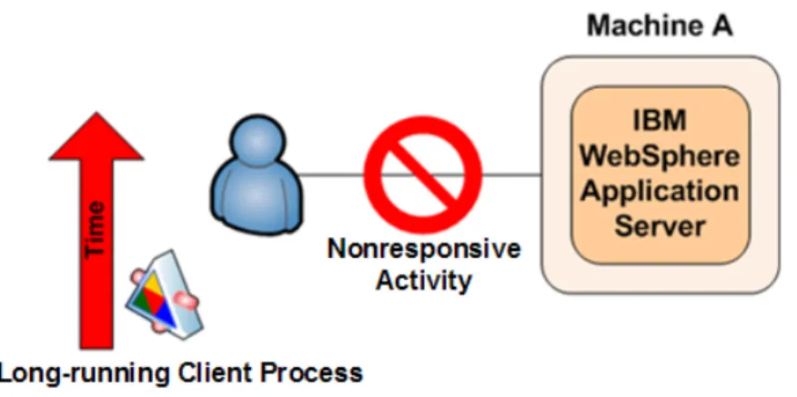
• Symptom: Long-running client process
• Middle-tier architecture: Intel, P4 Xeon processor, single Application Server
Figure 2. Client process experiences nonresponsive states during execution
The client in question experienced what appeared to be nonresponsive states during extended execution periods of a SAS solution. The WebSphere logs showed a corresponding java.lang.NullPointerException error during these periods of inactivity. Detailed analysis of the specified business scenario identified a single, long-running process that exceeded the default timeout constraints as defined within the WebSphere configuration. As a result, this process was forcibly closed. The resulting java.lang.NullPointerException error caused all downstream dependencies to be queued, pending successful completion of the cancelled job
The long-running process that was identified was a complex SQL query. Testing this query directly against the database showed close to a six-hour run time. The timeout was avoided by increasing the appropriate transaction-service options as follows:
The options were adjusted as follows:
1. Select Servers ► Application Servers ► server1 ►Transaction Service. 2. Set Total Transaction lifetime timeout to 21600.
3. Set Client inactivity timeout to 21600.
Because the job took six hours, the corresponding value in seconds is 21600. This is a good value for this specific scenario because it provides a sufficient amount of processing time for the job to complete without any timeouts. Note: In this example, other potential sources for the timeout were investigated and eliminated before finding the exact source of the problem.
Figure 3. Increasing appropriate transaction-service options resolves problem
JAVA MEMORY
This section provides a detailed discussion of how memory is assigned, limitations in the way memory is assigned, and how these limitations affect both the responsiveness and robustness of SAS solutions. This discussion is followed by a number of case studies. Memory that is assigned to the JVM is defined with the -Xms and -Xmx
command-line options. Table 2 shows these options and initial starting values that are suggested by SAS Technical Support.
JVM Initial Starting Values for -Xms and -Xmx Few users/Sun JVM -Xms512m -Xmx512m More users/Sun JVM -Xms1280m -Xmx1280m Few users/IBM JVM -Xms256m -Xmx512m More users/IBM JVM -Xms640m -Xmx1280m WebSphere 6.x – Windows (W32) -Xms640m -Xmx1472m WebSphere 6.x – AIX -Xms640m -Xmx1840m
WebSphere 6.x – Solaris (SPARC)
-Xms640m -Xmx1840m Table 2. Initial starting values for the -Xmx and –Xmx options
Before considering the impact of differing methods for internally managing memory, you must first consider how memory is allocated. Memory that is allocated to the JVM is dynamic, and it is dependent upon the settings that you give when you start the JVM. Such a dynamic allocation of memory is referred to as a heap. From this point forward, memory that is allocated to the JVM will be referred to as the Java heap. The Java heap must be a single contiguous allocation of memory; therefore, memory must be allocated in a single block.
The available Java heap is a concern because it has a major impact on the responsiveness and robustness of your SAS solution. When the Java heap is in use, the SAS Web application loads objects into the heap. For example, each live user session stores objects within the Java heap. However, the Java heap is a limited resource. If the JVM can no longer allocate objects to the Java heap, the JVM will crash with an out-of-memory error. Also, depending upon the size of the Java heap, the automatic memory-management process can start to consume significant system resources. This process then affects the responsiveness of the JVM and, in turn, the responsiveness of your SAS solution.
Before further consideration of the methods for defining the Java heap, some consideration must be given to the system limitations that are placed on the size of the Java heap. SAS solutions that run on the SAS 9.1.3 Enterprise Intelligence Platform only support the use of a 32-bit Java environment, irrespective of the underlying operating system. This 32-bit environment has a maximum address space of 4 GB per process. This 32-bit limit is then further reduced by operating system constraints.
In the case of 32-bit Microsoft Windows environments, the default behavior of the operating system splits the 4 GB of address space into two equal areas. The first 2-GB area is allocated for the application; the second 2-GB area is allocated to the operating system for the kernel. Within the application space, the process code is loaded at the bottom of the space. The application also has one or more threads, and each thread has an associated stack that is then allocated from the application space.
In addition, the JVM needs to link to a number of operating-system libraries. The JVM is a small executable file, and it is mostly comprised of dynamic link libraries (DLLs). Along with these operating-system libraries, the JVM links to a number of application libraries. In most instances, the application libraries are loaded at the bottom of the application space, and the operating-system libraries are loaded at the top of the space. This arrangement leaves a segment, known as the Native heap, between the area that contains the process codes, the thread stack, and the application libraries and the area that contains the operating-system libraries. You can allocate the Java heap into this space. Figure 4, presents this allocation of the 4-GB address space.
Figure 4. Default allocation of address space in 32-bit Microsoft Windows environments
Of the available 2 GB per process-application space, the theoretical maximum Java heap size is approximately 1.75 GB. In practice, this limit is further reduced by the requirement for Just-In-Time (JIT) compiled code to be stored within the application space. As a result, the upper limit on the Java heap is approximately 1.5 GB.
This 1.5 GB limit is in the default configuration of the 32-bit Windows environment. However, Microsoft has an option that enables you to split the 4 GB of address space into 3 GB for the application space and 1 GB for the operating-system space. This option is the /LARGEADDRESSAWARE switch, which is often referred to as the /3GB switch. Initially, this switch appears to make available an additional 1 GB of memory for the Java heap, providing an upper limit of 2.5 GB. However, this is not the case. Even with the switch enabled, the operating-system link libraries are loaded to a default base memory address. This means that the libraries still split the address space and that the Java heap cannot expand through them. That is, because the Java heap must be a single, contiguous block, it is still bounded by the operating-system libraries. Figure 5 illustrates this method of splitting of the address space.
Figure 5. Alternative allocation of address space in 32-bit Microsoft Windows environments
While the Java heap cannot use the additional address space, the JIT complied code can use the space. Although the upper limit for the Java heap cannot extend to 2.5 GB, in practice, it can extend to approximately 1.8 GB. Therefore, the use of the /3GB switch can increase the Java heap’s addressable memory by up to 0.3 GB.
This limitation in the address space for a 32-bit process does not occur on other operating systems such as IBM AIX and Sun Solaris. In these UNIX environments, a 32-bit process can access far more of the 4 GB addressable space. In practice, under UNIX, the upper bound for the Java heap can be extended close to 3.5 GB because the operating systems do not cause limitations as do Windows operating systems. However, the system administrators in a UNIX environment might place manual limitations on a process. Under UNIX, the administrator can use the ulimit command or the /etc/security/limits file to place these restrictions. If issues occur when the upper bound for the Java heap is set, you need to investigate those issues.
Given the system restrictions on the size of the Java heap, we now examine the methods for setting the size of the heap. Irrespective of the JVM used, whether Sun or IBM, the following two command-line options apply:
• -Xmsmemory-size—Sets the initial size of the heap. • -Xmxmemory-size—Sets the maximum size of the heap.
In this syntax, memory-size is a multiple of 1024. You can also append either k or K to indicate kilobytes, m or M for megabytes and g or G for gigabytes. Figure 6 illustrates the use of the two options.
Figure 6. Setting the Java heap size
The automatic memory-management process expands the size of the heap from the -Xms value up to the -Xmx value as additional memory requests are made. The inverse also occurs as objects are freed. The automatic process reduces the size of the heap as well. In addition, it is possible to set the values of -Xms and -Xmx to the same value. In such a situation, the Java heap is not resized by the automatic memory-management process. An example of this situation is illustrated in one of the following case studies.
MEMORY-ALLOCATION CASE STUDIES
The need for more memory is often obvious—you will see a java.lang.OutOfMemoryError error in your Java Web Application Server. Sometimes, however, memory problems are less obvious. You might note that your system is suddenly unresponsive when you put it under heavy loads such as creating a year-end report, making a long and complex query, or using a large number of client connections simultaneously. This second case generally happens when your system spends time paging (using virtual memory rather than actual RAM). It can also happen when your system spends too much time collecting garbage in order to find enough memory to run. As a result, t the CPU is heavily taxed. In fact, sometimes memory issues can even appear to be thread issues because WebSphere reports any long-running thread as nonresponsive. We have often found that as memory constraints are eased, reports of nonresponsive threads in the logs often become less of an issue or they disappear entirely.
Allocating memory can also be a balancing act. If you’re constrained by the amount of RAM available to you, either because of your operating system or your hardware, you need to make sure that the amount of memory that you want to allocate for your Java Web Application Server is actually available. Out-of-memory exceptions are common when you attempt to tweak the two primary memory options, -Xmx and -Xms.
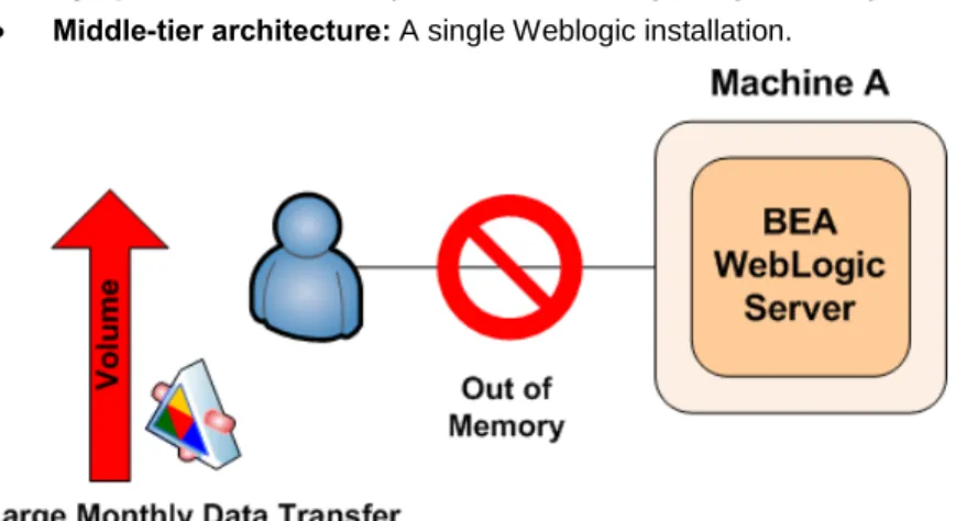
Case Study 1
• Symptom: Out-of-memory errors occur during a large, monthly data transfer. • Middle-tier architecture: A single Weblogic installation.
Figure 7. Out-of-memory exceptions occur during a large, monthly data transfer
For example, a multi-national electronics company was using SAS® Financial Management installed on a Windows middle-tier server. When they ran a large, monthly data transfer, out-of-memory exceptions appeared in their
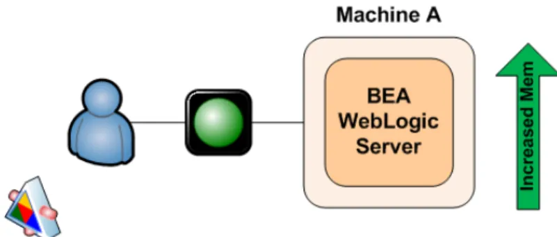
WebLogic server that was managed by the SAS® System. We suggested that they increase the values of -Xms and -Xmx by 50%. With these settings, the company could not bring up the managed server at all because we had exceeded the amount that could be allocated by the JVM on their operating system. We settled on setting both -Xms and -Xmx to 1024, which was a compromise that worked. The company was able to start its WebLogic server and execute their monthly data transfer without error.
Figure 8. Modifying the values of -Xms and -Xms resolves data-transfer problem
Case Study 2
• Symptom: NULL-pointer exceptions and an abnormal ending occur when running diagrams on data. • Middle-tier architecture: A single Weblogic installation.
Figure 9. Errors occur when a marketing diagram fails to run
An insurance company that was using a SAS solution encountered a NULL-pointer exception (NullPointerException) in the application log and an abnormal ending when a marketing diagram failed to run. The company was unable to send us a WebLogic log, but we suspected some sort of resource constraint because we knew that less complex diagrams had been run successfully on the same data. First, we tried adjusting timeout settings to see if that would make the diagram run consistently, but that did not work. Then, we focused on memory, which is generally the next constraint we consider. The company was already using the maximum amount of memory that could be allocated on its Windows 2003 Server Enterprise Edition without using the /3GB switch, so we suggested turning on the /3GB switch. Using this switch is not without cost. Operating-system overhead splits the address space, and the Java heap cannot expand through them. However, in this instance, we decided, cautiously, to try it. With the switch, the
customer was able to set -Xms1196m -Xmx1196m. Surprisingly, the values could not be set any higher without receiving the error Couldnotreserveenoughspacefor objectheap. The company said that other Java applications on its box were able to start with higher memory settings. Aha, a clue! The company was running numerous other JVMs that were also attempting to allocate the limited memory resources. At start up, a JVM requests a total of -Xms+ PermSize bytes from the operating system. If the operating system cannot supply that much memory, you receive the same errors that the insurance company received. The company’s other Java applications were taking up almost all of the available memory, so the operating system was unable to allocate what was needed. We asked the company to move some of the other Java applications to other machines. Then we use -Xms and -Xmx to increase the memory available to WebLogic, and the diagram ran successfully.
Figure 2. Moving some applications to other machines and increasing memory resolves problem Case Study 3
• Symptom: SAS® Web Report Studio ends abnormally
• Middle-tier architecture: Tomcat Java Web Application Server
In some cases, you might also need to balance the amount of memory that can be allocated to each thread within your Java Web applications against the allocations for -Xms /-Xmx and PermSize. Recently, as a customer site in the US, a SAS Installation Representative was performing a stress test for SAS Web Report Studio users. The representative found that he was getting frequent crashes in Tomcat. He noticed that there were a fairly large number of threads (323) at the time of the crashes. Looking at the amount of available memory, the representative realized that if he allocated the usual amount of memory per thread, the system would quickly run out of available memory. The consultant reduced the thread size (via the -Xss option) to 64K. The option -Xss sets the maximum native stack size for any thread. He also noted that the value for -Xmx was 1.2G, which could be reduced to free up more space for threads. Permanent space can also be reduced to free up space for threads. These changes increased the number of threads that can be created without overflowing memory, and they seem to have solved the problem. Note that it is possible that the consultant might see other problems (such as StackOverflow errors) later in the testing process because of reduced thread stack. The reduced values for -Xmx and PermSize might also cause out-of-memory errors, depending on the type of load at the customer site. We suggested that the representative continue profiling the JVM and monitoring the logs to ensure that the settings continued to be a good match for the usage patterns.
Figure 4. Reducing thread size and values for –Xmx and PermSize resolves problem Case Study 4
• Symptom: Performance degradation occurs toward the end of each week. • Middle-tier architecture: IBM AIX and one WebSphere Application Server
Figure 5. Performance of SAS solution degrades by the end of each week
Although memory-allocation options are useful, there are times that simply clearing the cache will free enough memory to improve performance or prevent downtime. This was the case for one of our banking customers. They found that the performance of their SAS solution slowed perceptibly toward the end of each week. The company had complex execution tasks and a sizable user base, and the staff found that restarting the Java Web Application Server daily sped up performance so much that it made the difference in being able to finish their nightly batch jobs.
Although these jobs ran under UNIX, clearing the cache is a trick that can work on other operating systems and other Web application servers as well. Because this solution is even easier than changing options, it is often a good place to start.
Figure 6. Clearing the cache resolves performance degradation
If you suspect that memory constraints might be causing slow performance at your site, we suggest that you turn on garbage-collection logging for more detailed information. See the next section for a detailed discussion of garbage collection.
GARBAGE COLLECTION
This section covers several topics related to the automatic memory-management process (or, garbage collection): • key command-line options for garbage collection
• details of the garbage-collection process
• an explanation of how to set correct logging and tools for processing such logs. The last part of this section presents some case studies that deal with the garbage collection.
COMMAND-LINE OPTIONS FOR GARBAGE COLLECTION
As with the allocation of memory to the JVM, the automatic memory-management process has a number of key command-line options. These options are more extensive than those for memory allocation, so they are split into three tables. Error! Reference source not found. and Error! Reference source not found. present size and process-based options along with the recommended initial settings for the range of Java Web Application Servers.
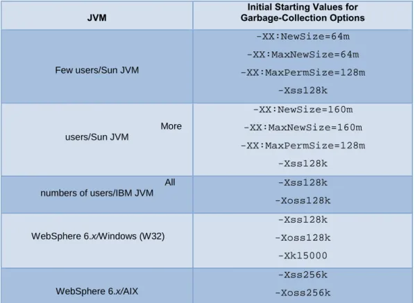
Table 3. Initial starting values of size-based, command-line options for garbage collection
JVM
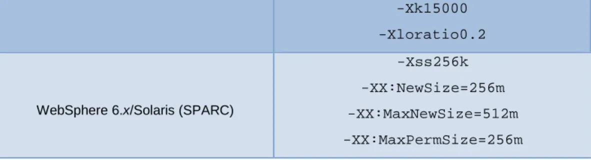
Initial Starting Values for Garbage-Collection Options Few users/Sun JVM -XX:NewSize=64m -XX:MaxNewSize=64m -XX:MaxPermSize=128m -Xss128k More users/Sun JVM -XX:NewSize=160m -XX:MaxNewSize=160m -XX:MaxPermSize=128m -Xss128k All numbers of users/IBM JVM -Xss128k -Xoss128k WebSphere 6.x/Windows (W32) -Xss128k -Xoss128k -Xk15000 WebSphere 6.x/AIX -Xss256k -Xoss256k
-Xk15000 -Xloratio0.2
WebSphere 6.x/Solaris (SPARC)
-Xss256k -XX:NewSize=256m -XX:MaxNewSize=512m -XX:MaxPermSize=256m
Table 4. Initial starting values of process-based, command-line options for garbage collection JVM Initial Starting Values for Command-Line Options
All numbers of users/Sun JVM
-XX:-UseTLAB -XX:+UseConcMarkSweepGC -XX:+DisableExplicitGC -Dsun.rmi.dgc.client.gcInterval=3600000 -Dsun.rmi.dgc.server.gcInterval=3600000 Few users/IBM JVM -Xpartialcompactgc -Xgcpolicy:optthruput -Dsun.rmi.dgc.client.gcInterval=3600000 -Dsun.rmi.dgc.server.gcInterval=3600000 WebSphere 6.x/Windows (W32) -Xpartialcompactgc -Xgcpolicy:optthruput -Dsun.rmi.dgc.client.gcInterval=3600000 -Dsun.rmi.dgc.server.gcInterval=3600000 -Dsun.rmi.dgc.ackTimeout=1 WebSphere 6.x/AIX -Xpartialcompactgc -Xgcpolicy:optthruput -Dsun.rmi.dgc.client.gcInterval=3600000 -Dsun.rmi.dgc.server.gcInterval=3600000 -Dsun.rmi.dgc.ackTimeout=1
WebSphere 6.x/Solaris (SPARC)
-XX:+UseConcMarkSweepGC
-Dsun.rmi.dgc.client.gcInterval=3600000 -Dsun.rmi.dgc.server.gcInterval=3600000
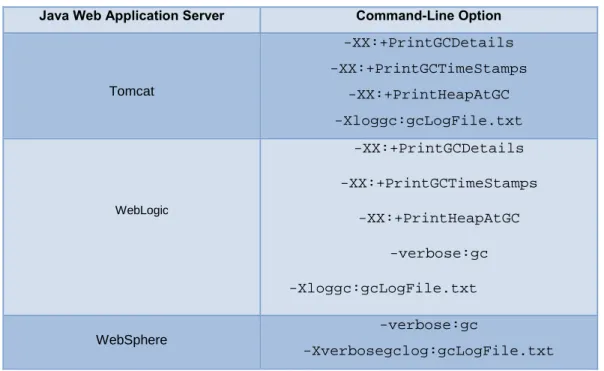
Table 5 presents the command-line options that you can use to enable specific logging for the automatic memory-management process.
Table 5. Garbage-collection logging options
Java Web Application Server Command-Line Option
Tomcat -XX:+PrintGCDetails -XX:+PrintGCTimeStamps -XX:+PrintHeapAtGC -Xloggc:gcLogFile.txt WebLogic -XX:+PrintGCDetails -XX:+PrintGCTimeStamps -XX:+PrintHeapAtGC -verbose:gc -Xloggc:gcLogFile.txt WebSphere -verbose:gc -Xverbosegclog:gcLogFile.txt
These initial settings are based on extensive testing by our performance testing group. For example, instead of using the default value 60000 (60 seconds) as the interval for distributed garbage collection, we specify the following:
-Dsun.rmi.dgc.client.gcInterval=3600000 -Dsun.rmi.dgc.server.gcInterval=3600000
The majority of SAS applications use the Java Remote Method Invocation (RMI), which, in turn uses distributed garbage collection. Our testing has found that the default value results in excessive overhead in a SAS enterprise business intelligence system. A value of 3600000 (60 minutes) provides better throughput.
We have changed our recommendation with regard to the -Xnoclassgc (disable class garbage collection) option. In older JVMs (1.4.x), use of this (non-default) option was beneficial for shorter runs. The default garbage-collection action for a JVM is to collect classes. This action provides a somewhat smaller memory footprint at the cost of higher overhead from loading and unloading classes. With class garbage-collection turned off, the system had better throughput and better overall performance on older JVMs with smaller loads. Recent endurance tests have shown that it is better for continuously heavy-loaded systems if the JVM collect the classes, even with the older JVMs. It is even truer in more recent versions of the JVM, in which the collection of classes is more efficient. Because of this (and regardless of the JVM), the current recommendation for most SAS customers is that they do not use the -Xnoclassgc option.
GARBAGE-COLLECTION PROCESS
Garbage-collection methodology is one of the greatest differences between the Sun and IBM JVMs. The Java specification only states that the garbage-collection process must be enacted on the Java heap, but it does not state how the garbage-collection process should function. The garbage-collection process, at its simplest, must have two phases. In the first phase, the process must analyze the objects in the heap to identify those that are no longer being referenced. In the second phase, the process must clear the space that is used by those objects. An object is considered to be garbage when it can no longer be reached from any pointer in the running program.
The Sun JVM uses a generation model for garbage collection. Generational garbage collection exploits the following, empirically observed properties of most applications to simplify the process:
• The majority of objects exist for a very short time. • Some objects exist for the lifetime of an application.
• A minority of objects exist for the duration of some intermediate computation.
For the generational model, memory is managed in a generation, which is a pool that holds objects of different ages. Garbage collection then occurs in each pool as that pool fills up. Objects are initially allocated in a generation for younger objects. This generation is called the Young generation. When this generation is full, it causes a minor
garbage collection, which is only a collection of part of the Java heap. Because the majority of objects only exist for a short time, these minor collections can be optimized, assuming that the majority of objects are not still being used. Figure 7 presents the layout of the Sun generational heap structure, where the virtual sections account for the expansion that is available when the value of -Xmx is greater than the value of -Xms.
Figure 7. Sun generational JVM heap structure
The Young generation shown in Figure 15 consists of three disparate pool areas: the first area is Eden; the other two, equally-sized, Survivor spaces called FROM and TO. The objects are initially allocated in Eden. When the Eden space fills, the minor garbage collection clears the unreferenced objects. Objects that survive this collection are moved to the FROM survivor space. Once the garbage collection is complete, the pointers on the two survivor spaces are reversed: TO becomes FROM, and FROM becomes TO.
The Young generation is sized with the -XX:NewSize and -XX:MaxNewSize options on the command line. The -XX:NewSize option sets the initial size, and the –XX:MaxNewSize option provides an upper bound. The Young generation should never exceed half of the Java heap; by default, this is set to one-half of the Java heap if the heap is less than 1.5 GB and to one-third of the Java heap is the heap is larger than 1.5 GB. The Survivor space in the Young generation is sized as a ratio of one of the sub-spaces to the Eden space; this is referred to as the SurvivorRatio. The total size of the Young generation will equal Eden space plus the two Survivor spaces. Because the SurvivorRatio refers only to one of the Survivor spaces, you can see that Young = (SurvivorRatio + 2) x (Size of one Survivor sub-space). Therefore, if Young = 600m and -XX:SurvivorRatio=4, then the value for each Survivor sub-space is 100m, and the value for the Eden space is be 400m.
Once an object survives a number of minor garbage collections, it is tenured from the TO Survivor space to the Tenured generation. Objects in the Tenured space are only collected if a full garbage collection occurs. If the Tenured space is full and the garbage collection cannot expand the Java heap, an out-of-memory error occurs and the JVM crashes. As detailed previously, you size the Tenured space with the –Xms and –Xmx command-line options.
The Permanent space is where class files are stored. These class files are the results of compiled classes and JSP pages. If this space is full, then a major garbage collection occurs. As is the case in the Tenured space, if the garbage collection cannot clear part of this space, an out-of-memory error occurs and the JVM crashes. You size the Permanent space with the command-line options -XX:PermSize and -XX:MaxPermSize. The first option specifies the initial size; the second option specifies the upper bound. For example, the following options specify a startup Permanent space of 48 MB and a maximum Permanent space size of 128 MB:
-XX:PermSize=48m –XX:MaxPermSize=128m
Note that the Permanent space is in addition to the Java heap. Therefore, the total initial space is -Xms+-XX:PermSize, and that the maximum space is –Xmx + -XX:MaxPermSize.
Irrespective of the detail of the minor and major garbage-collection routines, tuning the size of the generation spaces within the Java heap that is used by the Sun JVM will impact the responsiveness and robustness of the SAS solution. If the Permanent space is too small, for example, the JVM can crash. If the Permanent space is too large, there will be insufficient space for the Young and Tenured generations. If the Young generation is too small, garbage collection will be more frequent, which will reduce the responsiveness of the SAS solution.
The Sun JVM has two main garbage-collection routines, minor and major. The minor garbage collection occurs when the Eden space is full. By default, this process is single threaded, but it does not interrupt any other threads that are working on objects within the JVM. Later in this section, the options for parallelizing the minor garbage-collection process are discussed.
Major, or full, garbage collection occurs when either the Tenured or Permanent spaces are full. If the initial and maximum sizes of these two spaces are different, then the full garbage collection increases these spaces toward their maximum sizes. You can avoid this process by setting -Xms and -Xmx to the same value and setting -XX:PermSize and -X:MaxPermSize to the same value. Similarly, you can tune the size of the Young generation such that more objects are filtered out before they are tenured. Full garbage collection is disruptive in the sense that all working threads are stopped, while one JVM thread then scans then entire heap twice in an attempt to clean out unreferenced objects. This activity can cause delays in response time for the JVM. The aim of tuning the JVM is to minimize the major garbage collections while ensuring that an out-of-memory error does not crash the JVM.
The Sun JVM has four types of garbage collector. Up to this point, all discussion has been about the default collector. The additional three collectors are as follows:
• Throughput collector(-XX:+UseParallelGC)—Uses a parallel version of the Young Generation collector. The Tenured-generation collector is the same as the default collector. You should use this collector when you are trying to improve the responsiveness of a SAS solution by making use of a larger number of processors. As mentioned previously, the default collector uses a single thread; therefore, garage collection adds to the overall execution time of the application. The throughput collector uses multiple threads to execute a minor collection, thereby reducing the overall execution time of the application. The number of garbage-collection threads can be controlled with the -XX:ParallelGCThreads command-line option. • Concurrent low-pause collector (-XX:+UseConcMarkSweepGC)—Collects the Tenured generation
and does most of the collection concurrently with the execution of the application. The application is only paused for short periods during the collection. A parallel version of the Young-generation copying collector is used with the concurrent collector. You can use the concurrent low-pause collector if your application will benefit from shorter garbage-collector pauses and if the application can share processor resources with the garbage collector when the application is running. This is typical of applications that have a relatively large set of long-lived data and that run on machines with two or more processors.
• Incremental low-pause collector (-Xincgc)—Collects just a portion of the Tenured generation at each minor collection, attempting to spread the large pause of a major collection over many minor collections. You can use this collector when your application can afford to trade longer and more frequent Young-generation collection pauses for shorter Tenured-generation pauses.
The IBM JVM used by IBM WebSphere has different methods of handling garbage collection than those used by the Sun JVM. As discussed previously, the Sun JVM uses the notion of age and, therefore, is referred to as a
generational model. The IBM JVM does not use the notion of age. Instead, it focuses on the type of object that requires space within the Java heap. As such, the IBM JVM uses a monolithic model for garbage collection. This difference in underlying models for garbage collection leads to a very different structure for the Java heap. Figure 8
illustrates the layout of the IBM JVM heap structure.
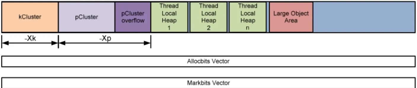
Figure 8. IBM JVM heap structure
In this structure, specific types of objects are stored within the first two areas of the IBM Java heap. The first area, called the kCluster, stores classes. The second area (pCluster) stores objects that should not be moved during a garbage collection. The rest of the IBM Java heap is used to store other objects that require space. Within these sections, objects are placed based upon their size rather than on a notion of age. The smallest objects are stored within thread-specific areas of the heap. Each thread has its own specific storage area as opposed to each thread creating objects within the Eden space. The largest objects are stored within the Large Object Are, and all other objects are stored generally within the remaining space. Clearly this monolithic model is very different from the Sun generational model.
Now, we will examine the IBM memory management process in more detail. The SAS Web application suite uses a high number of classes, which makes fragmentation of the heap a concern. This concern can be addressed by tuning the kCluster and the pCluster, which are at the base of the Java heap. The kCluster stores class blocks, and it is sized with the -Xk command-line option. By default, this space is sufficient for 1280 class blocks, where each class block is approximately 300 bytes long. The -Xk option takes an argument that specifies the maximum number of classes that the kCluster will contain.
For most objects within the heap, the locations of objects are not important and the garbage-collection routine can move these objects about within the heap. However, some objects cannot be moved, either temporarily or
permanently. Such objects are referred to as pinned objects. The pCluster allocates space for these pinned objects. In addition, the pCluster also stores class blocks when the kCluster is fully allocated. Once the pCluster is fully allocated, the garbage-collection routine assigns an additional pCluster. The pCluster is sized with the -Xp command-line option, this can take two arguments. The first argument specifies the initial cluster size, and the second argument specifies the overflow cluster size. The overflow cluster size is the size of the subsequent pClusters that are created by the garbage-collection routine. Both arguments are specified in bytes, and they can take K or M
suffixes to signify kilobytes or megabytes. For example, -Xp16K,2K sets an initial size of 16 kilobytes, with an overflow of 2 kilobytes.
In addition to the Java heap, the IBM JVM also creates the allocbits and markbits vectors. The allocbits vector is a flag that signifies that an area of the heap has been allocated. The markbitsvector is part of the garbage-collection routine. The garbage-collection routine carries three phases; mark, sweep, and (optionally) compaction. During the mark phase, if an allocated object within the heap is referenced, the garbage-collection routine sets a flag within the markbits vector.
As a memory-management process, the garbage-collection routine also handles memory allocation. Because the allocation of memory is a much simpler process, the term garbage collection is used to cover the whole process. The allocation of an object requires a heap lock to prevent concurrent-thread access to the heap. To optimize the allocation process, areas of the heap are set aside as thread-specific caches. Such a cache is referred to as a Thread Local Heap. Because a cache is specific to an individual thread, a heap lock is not required when objects are allocated. This provides the best performance for the allocation of small objects. Small objects are directed to the end of the Thread Local Heap. Currently, the Thread Local Heap is only used for objects smaller than 512 bytes.
If objects cannot be allocated through either the Thread Local Heap or the general heap lock, they will be allocated into the Large Object Area. Before a garbage collection, objects are allocated from first half of the Large Object Area. After a garbage collection, if the only space large enough to satisfy the allocation request is in the Large Object Area, the allocation is made from the second half of the Large Object Area. You can use the -Xloratio command-line option to size the Large Object Area. The –Xloratio command takes an argument that specifies the fraction of the Java heap, in the range 0.5 to 0.95, to reserve for the Large Object Area. So, for example, to reserve 30% for the Large Object Area, command is -Xlorato0.3. SAS recommends an initial value of -Xloratio0.2, corresponding to 20%.
The IBM garbage-collection routine is a stop-the-world routine, which means that the thread that carries out the garbage collection first gets all of the locks that are required for the garbage collection and then suspends all the other threads. Garbage collection then goes through the three phases: mark, sweep, and (optionally) compaction. In the mark phase, all reachable objects are marked, and the mark is placed in the markbits vector. If an object is not reachable, then it must be garbage.
After the mark phase, the markbits vector contains a bit for every reachable object, and the vector must be a subset of the allocbits vector. The sweep phase identifies the intersection of the markbits and allocbits vectors, which contains all objects that are allocated but are not referenced. Then the collector identifies sequences of zeros that match a segment of the heap that can be freed. The collector then checks the size of the space. If the size is greater than 512 bytes, that space is put on the free list so it can be reallocated. If the size is not greater than 512 bytes, the space is referred to as dark matter, and it is freed when the space next to it becomes free. Finally, the markbits vector is copied onto the allocbits vector so that the allocbits vector correctly identifies allocated objects on the heap.
The final phase, compaction, is optional. Once the garbage is cleared and that space is returned to the free list, referenced objects are scattered around the heap. The compaction phase looks to move all of the objects in such a way that the free space is in a continuous block. This is a complicated procedure because if an object is moved, the garbage collector must update all references to the moved object. Some objects cannot be moved.
As with the Sun JVM, the IBM JVM has the following additional options you can use to improve the garbage-collection process:
• Parallel Mark—Provides a parallel version of the garbage-collector mark phase because considerable time can be taken confirming if each object in the heap can be referenced. Further discussion of the threading capabilities of the garbage collector will be covered in the next section.
• Concurrent Mark—Provides shorter and more consistent times for the mark phase as the overall size of the Java heap increases. This is achieved because the concurrent mark process starts before the heap is full and the main garbage collection is called. Tracing is performed by a low-priority background thread and by each application thread when it does a heap-lock allocation. The garbage collector tries to start the concurrent mark phase so that it completes at the same time that the heap is exhausted. The garbage collector does this by constant tuning of the options that govern the concurrent mark time. The commandline option
-Xgcpolicy, controls the use of Concurrent Mark. Setting -Xgcpolicy:optthruput disables
Concurrent Mark, while setting -Xgcpolicy:optavgpause enables Concurrent Mark. Concurrent Mark carries a cost in the form of the additional work each application thread is required to do.
• Parallel Sweep,Provides a parallel version of the garbage-collector sweep and uses the same additional threads to carry out the sweep phase.
• IncrementalCompaction—Splits the heap into sections and compacts each section as it would with a full compaction. That is, the garbage collector moves all moveable objects down the heap. This action retrieves the dark-matter space and leaves large sections of free space. Incremental compaction operates
successively over a number of garbage-collection cycles. Cycling spreads the compaction time over multiple garbage collections, thereby reducing pause times. You can enable incremental compaction for every garbage-collection cycle with the command-line option –Xpartialcompactgc. To disable it for the life of the JVM, use -Xnopartialcompactgc.
As you can see, the Sun and IBM JVMs have two very different methodologies for automatic memory management. Along with the two models, generational and monolithic, there are a number of different settings you can modify to optimize the performance of the JVM and improve both the responsiveness and robustness of your SAS solution. Given this wide range of settings for the garbage collection, it becomes important to obtain as much information as possible regarding the behavior of the garbage-collection algorithms. You can obtain far more information than that outputted by the monitoring tools reviewed earlier by enabling the garbage-collection logging, as explained in the next section.
SETTING GARBAGE-COLLECTION LOGGING
If you get out-of-memory errors, we recommend that you gather information about the garbage collection that is being performed for your Web application server. This information can help pinpoint where the memory problem is
occurring. To obtain this information, set the following command-line options, and then stress the system to re-create the errors:
For Tomcat, add these JVM command-line options to each instance: -XX:+PrintGCDetails
-XX:+PrintGCTimeStamps -XX:+PrintHeapAtGC -Xloggc:gcLogFile.txt
The JVM overwrites the log file each time it starts, so be sure to retain a copy of the log file before you restart the JVM. We also recommend that you give the log file for each instance a unique name so that you can keep them straight.
To debug garbage-collection and memory problems on WebLogic, add the following command-line options: -XX:+PrintGCDetails
-XX:+PrintGCTimeStamps -XX:+PrintHeapAtGC -verbose:gc
-Xloggc:gcLogFile.txt If the following option is present, remove it:
-XX:+UseConcMarkSweepGC
The -Xloggc option can be a fully qualified path rather than a simple file name. Restart the WebLogic instance in order for the additional command-line options to take effect.
To enable garbage-collection logging in WebSphere Versions 5.1 and 6.x, perform the following steps: 1. In the Administrative Client, expand Servers and then click Application Servers. 2. Click the server of interest.
3. Under the Additional Properties section, click Process Definition. 4. Under the Additional Properties section, click Java Virtual Machine. 5. Select the Verbose garbage collection check box.
6. Click Apply.
7. At the top of the Administrative Client, click Save to save the changes to your configuration. 8. Stop and start the application server.
After you complete these steps, the verbose garbage-collection output is written to the native_stderr.log. The previous steps performed in the administrative console add the -verbose:gc option to the JVM. The IBM JVM provides extensive memory tracing with this option set. Alternatively, you can use the -verbosegclog:LogFile.txt command-line option..
Output from the garbage-collection logging is not straightforward to review. A number of tools are available to assist you in the analysis of the garbage-collection logs. One such tool, Tagtraum Industries’ GCViewer, is an open-source,
Java application that enables you to analyze the logs from both the Sun and IBM JVMs. More information regarding GCViewer is available from Tagtraum Industries’ Web site. Because GCViewer is a Java application, it consumes system resources just like the Java Web Application Server does. Therefore, you should not perform an analysis of results on the same machine that runs your Java Web Application Server. Display 4 illustrates sample output in the GCViewer application.
Display 4. Sample output from the GCViewer application
The IBM Pattern Modeling and Analysis Tool for the Java Garbage Collector (PMAT) is an alternative application that you can use. This application is available from www.alphaworks.ibm.com/tech/pmat. As defined on the IBM
AlphaWorks site, the PMAT application parses verbose garbage-collection tracings, analyzes Java heap use, and recommends key configurations based on pattern modeling of Java heap use.
Display 5 illustrates sample output that is provided by the PMAT tool when you analyze the output from a WebSphere Java Application server log file.