Oracle White Paper June 2013
Optimizer
Disclaimer
The following is intended to outline our general product direction. It is intended for information purposes only, and may not be incorporated into any contract. It is not a commitment to deliver any material, code, or functionality, and should not be relied upon in making purchasing decisions. The development, release, and timing of any features or functionality described for Oracle’s products remains at the sole discretion of Oracle.
Introduction ... 2
New Optimizer and statistics features... 3
Adaptive Query Optimization ... 3
Optimizer statistics... 16
New Optimization Techniques ... 24
Enhancements to existing functionality... 29
SQL Plan Management... 29
Statistics enhancements ... 32
Introduction
The optimizer is one of the most fascinating components of the Oracle Database, since it is essential to the processing of every SQL statement. The optimizer determines the most efficient execution plan for each SQL statement based on the structure of the given query, the available statistical information about the underlying objects, and all the relevant optimizer and execution features.
With each new release the optimizer evolves to take advantage of new functionality and the new statistical information to generate better execution plans. Oracle Database 12c makes this evolution go a step further with the introduction of a new adaptive approach to query
optimizations.
This paper introduces all of the new optimizer and statistics related features in Oracle
Database 12c and provides simple, reproducible examples to make it easier to get aquatinted with them. It also outlines how existing functionality has been enhanced to improve both performance and manageability.
New Optimizer and statistics features
Adaptive Query Optimization
By far the biggest change to the optimizer in Oracle Database 12c is Adaptive Query Optimization. Adaptive Query Optimization is a set of capabilities that enable the optimizer to make run-time adjustments to execution plans and discover additional information that can lead to better statistics. This new approach is extremely helpful when existing statistics are not sufficient to generate an optimal plan. There are two distinct aspects in Adaptive Query Optimization, adaptive plans, which focuses on improving the initial execution of a query and adaptive statistics, which provide additional information to improve subsequent executions.
Figure 1. The components that make up the new Adaptive Query Optimization functionality Adaptive Plans
Adaptive plans enable the optimizer to defer the final plan decision for a statement, until execution time. The optimizer instruments its chosen plan (the default plan), with statistics collectors so that at runtime, it can detect if its cardinality estimates, differ greatly from the actual number of rows seen by the operations in the plan. If there is a significant difference, then the plan or a portion of it can be automatically adapted to avoid suboptimal performance on the first execution of a SQL statement.
Adaptive Join Methods
The optimizer is able to adapt join methods on the fly by predetermining multiple subplans for portions of the plan. For example, in Figure 2 the optimizer’s initial plan choice (default plan) for joining the order_items and product_info tables is a nested loops join via an index access on the product_info table. An alternative subplan, has also been determined that allows the optimizer to switch the join type to a hash join. In the alternative plan the product_info table will be accessed via a full table scan.
During execution, the statistics collector gathers information about the execution and buffers a portion of rows coming into the subplan. In this example, the statistics collector is monitoring and buffering rows coming from the full table scan of order_items. Based on the information seen in the
statistics collector, the optimizer will make the final decision about which subplan to use. In this case, the hash join is chosen as the final plan since the number of rows coming from the order_items table is larger than the optimizer initially estimated. After the optimizer chooses the final plan, the statistics collector stops collecting statistics and buffering rows, and just passes the rows through instead. On subsequent executions of the child cursor, the optimizer disables buffering, and chooses the same final plan. Currently the optimizer can switch from a nested loops join to a hash join and vice versa. However, if the initial join method chosen is a sort merge join no adaptation will take place.
Figure 2. Adaptive execution plan for the join between the Order_items and Prod_info tables
By default, the explain plan command will show only the initial or default plan chosen by the
optimizer. Whereas the DBMS_XPLAN.DISPLAY_CURSOR function displays only the final plan used by the query.
To see all of the operations in an adaptive plan, including the positions of the statistics collectors, the additional format parameter ‘+adaptive’ must be specified in the DBMS_XPLAN functions. In this mode
an additional notation (-) appears in the id column of the plan, indicating the operations in the plan that were not used (inactive). The SQL Monitor tool in Oracle Enterprise Manager always shows the full adaptive plan but does not indicate which operations in the plan are inactive.
Figure 4. Complete adaptive plan displayed using ‘+adaptive’ format parameter in DBMS_XPLAN.DISPLAY_CURSOR
A new column has also been added to V$SQL(IS_RESOLVED_ADAPTIVE_PLAN) to indicate if a SQL statement has an adaptive plan and if that plan has been full resolved or not. If
IS_RESOLVED_ADAPTIVE_PLAN is set to ‘Y’, it means that the plan was not only adaptive, but the
final plan has been selected. However, if IS_RESOLVED_ADAPTIVE_PLAN is set to ‘N’, it indicates the plan selected is adaptive but the final plan has not yet been decided on. The ‘N’ value is only possible during the initial execution of a query, after that the value for an adaptive plan will always be ‘Y’. This column is set to NULL for non-adaptive plans.
It is also possible to put adaptive join methods into reporting mode by setting the initialization parameter OPTIMIZER_ADAPTIVE_REPORTING_ONLY to TRUE (default FALSE). In this mode,
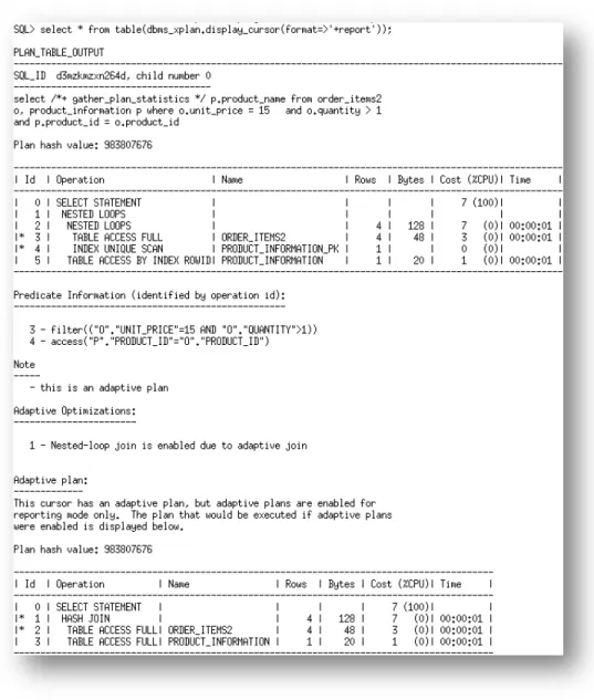
information needed to enable adaptive join methods is gathered, but no action is taken to change the plan. This means the default plan will always be used but information is collected on how the plan would have adapted in non-reporting mode. This information can be viewed in the adaptive plan report, which is visible when you display the plan using the additional format parameter ‘+report’.
Figure 5. Complete adaptive report displayed using ‘+report’ format parameter in DBMS_XPLAN.DISPLAY_CURSOR
Adaptive Parallel Distribution Methods
When a SQL statement is executed in parallel certain operations, such as sorts, aggregations, and joins require data to be redistributed among the parallel server processes executing the statement. The distribution method chosen by the optimizer depends on the operation, the number of parallel server processes involved, and the number of rows expected. If the optimizer inaccurately estimates the number of rows, then the distribution method chosen could be suboptimal and could result in some parallel server processes being underutilized.
With the new adaptive distribution method, HYBRID HASH the optimizer can defer its distribution method decision until execution, when it will have more information on the number of rows involved. A statistics collector is inserted before the operation and if the actual number of rows buffered is less
than the threshold the distribution method will switch from HASH to BROADCAST. If however the number of rows buffered reaches the threshold then the distribution method will be HASH. The threshold is defined as 2 X degree of parallelism.
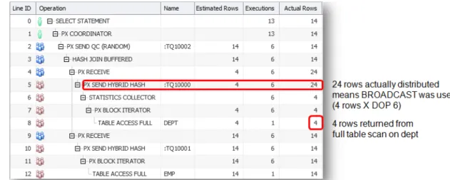
Figure 6 shows an example of a SQL Monitor execution plan for a join between EMP and DEPT that is executed in parallel. One set of parallel server processes (producers or pink icons) scan the two tables and send the rows to another set of parallel server processes (consumers or blue icons) that actually do the join. The optimizer has decided to use the HYBRID HASH distribution method. The first table accessed in this join is the DEPT table. The rows coming out of the DEPT table are buffered in the statistics collector, on line 6 of the plan, until the threshold is exceeded or the final row is fetched. At that point the optimizer will make its decision on a distribution method.
Figure 6. SQL Monitor execution plan for hash join between EMP & DEPT that uses adaptive distribution method Let’s assume the degree of parallelism in this example was set to 6 and the number of rows returned from the scan of the DEPT table is 4, the threshold would be 12 rows (2 X 6). Since the threshold was not reached, the 4 rows returned from the DEPT table will be BROADCAST to each of the 6 parallel server processes responsible for completing the join, resulting in 24 rows (4 X 6) being processed by the distribution step in the plan (see figure 7). Since a BROADCAST distribution was used for rows coming from the DEPT table, the rows coming from the EMP table will distributed via ROUND-ROBIN. This means, one row from the EMP table will be sent to each of the 6 parallel server processes in turn, until all of the rows have been distributed.
Figure 7. HYBRID-HASH distribution using BROADCAST distribution because threshold not reached
However, if the degree of parallelism in this example was set to 2 and the number of rows returned from the scan of the DEPT table was 4, the threshold would be 4 rows (2 X 2). Since the threshold was reached, the 4 rows returned from the DEPT table will be distributed by HASH among the 2 parallel server processes responsible for completing the join, resulting in just 4 rows being processed by the distribution step in the plan (see figure 8). Since a HASH distribution was used for rows coming from the DEPT table, the rows coming from the EMP table will also be distributed via HASH.
Figure 8. HYBRID-HASH distribution using HASH distribution because threshold was reached Adaptive Statistics
The quality of the execution plans determined by the optimizer depends on the quality of the statistics available. However, some query predicates become too complex to rely on base table statistics alone and the optimizer can now augment these statistics with adaptive statistics.
Dynamic statistics
During the compilation of a SQL statement, the optimizer decides if the available statistics are sufficient to generate a good execution plan or if it should consider using dynamic sampling. Dynamic sampling is used to compensate for missing or insufficient statistics that would otherwise lead to a very bad plan. For the case where one or more of the tables in the query does not have statistics, dynamic sampling is used by the optimizer to gather basic statistics on these tables before optimizing the statement. The statistics gathered in this case are not as high a quality (due to sampling) or as complete as the statistics gathered using the DBMS_STATS package.
In Oracle Database 12c dynamic sampling has been enhanced to become dynamic statistics. Dynamic statistics allow the optimizer to augment existing statistics to get more accurate cardinality estimates for not only single table accesses but also joins and group-by predicates. A new level, 11 has also been introduced for the initialization parameter OPTIMIZER_DYNAMIC_SAMPLING. Level 11 enables the
optimizer to automatically decide to use dynamic statistics for any SQL statement, even if all basic table statistics exist. The optimizer bases its decision, to use dynamic statistics, on the complexity of the predicates used, the existing base statistics, and the total execution time expected for the SQL statement. For example, dynamic statistics will kick in for situations where the Optimizer previously would have used a guess. For example, queries with LIKE predicates and wildcards.
Figure 9. When OPTIMIZER_DYNAMIC_SAMPLING is set to level 11 dynamic sampling will be used in stead of guesses
Given these new criteria it’s likely that when set to level 11, dynamic sampling will kick-in more often than it did before. This will extend the parse time of a statement. In order to minimize the
performance impact, the results of the dynamic sampling queries will be persisted in the cache, as dynamic statistics, allowing other SQL statements to share these statistics. SQL plan directives, which are discussed in more detail below, also take advantage of this level of dynamic sampling.
Automatic Reoptimization
In contrast to adaptive plans, automatic reoptimization changes a plan on subsequent executions after the initial execution. At the end of the first execution of a SQL statement, the optimizer uses the information gathered during the initial execution to determine whether automatic reoptimization is worthwhile. If the execution information differs significantly from the optimizer’s original estimates, then the optimizer looks for a replacement plan on the next execution. The optimizer will use the information gathered during the previous execution to help determine an alternative plan. The optimizer can reoptimize a query several times, each time learning more and further improving the plan. Oracle Database 12c supports multiple forms of reoptimization.
Statistics feedback
Statistics feedback (formally known as cardinality feedback) is one form of reoptimization that automatically improves plans for repeated queries that have cardinality misestimates. During the first execution of a SQL statement, the optimizer generates an execution plan and decides if it should enable statistics feedback monitoring for the cursor. Statistics feedback is enabled in the following cases: tables with no statistics, multiple conjunctive or disjunctive filter predicates on a table, and predicates containing complex operators for which the optimizer cannot accurately compute cardinality estimates.
At the end of the execution, the optimizer compares its original cardinality estimates to the actual cardinalities observed during execution and, if estimates differ significantly from actual cardinalities, it stores the correct estimates for subsequent use. It will also create a SQL plan directive so other SQL statements can benefit from the information learnt during this initial execution. If the query executes again, then the optimizer uses the corrected cardinality estimates instead of its original estimates to determine the execution plan. If the initial estimates are found to be accurate no additional steps are taken. After the first execution, the optimizer disables monitoring for statistics feedback.
Figure 10 shows an example of a SQL statement that benefits from statistics feedback. On the first execution of this two-table join, the optimizer underestimates the cardinality by 8X due to multiple, correlated, single-column predicates on the customers table.
After the initial execution the optimizer compares its original cardinality estimates to the actual number of rows returned by the operations in the plans. The estimates vary greatly from the actual number of rows return, so this cursor is marked IS_REOPTIMIZIBLE and will not be used again. The
IS_REOPTIMIZIBLE attribute indicates that this SQL statement should be hard parsed on the next
execution so the optimizer can use the execution statistics recorded on the initial execution to determine a better execution plan.
Figure 11. Cursor marked IS_REOPTIMIZIBLE after initial execution statistics vary greatly from original cardinality estimates
A SQL plan directive is also created, to ensure that the next time any SQL statement that uses similar predicates on the customers table is executed, the optimizer will be aware of the correlation among these columns.
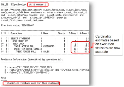
On the second execution the optimizer uses the statistics from the initial execution to determine a new plan that has a different join order. The use of statistics feedback in the generation of execution plan is indicated in the note section under the execution plan.
The new plan is not marked IS_REOPTIMIZIBLE, so it will be used for all subsequent executions of this SQL statement.
Figure 13. New plan generated using execution statistics from initial execution
Performance feedback
Another form of Reoptimization is Performance Feedback, which helps to improve the degree of parallelism chosen for repeated SQL statements when Automatic Degree of Parallelism (AutoDOP)1 is
enabled in adaptive mode.
When AutoDOP is enabled in adaptive mode, during the first execution of a SQL statement, the optimizer determines if the statement should execute in parallel and if so what parallel degree should be used. The parallel degree is chosen based on the estimated performance of the statement.
Additional performance monitoring is also enabled for the initial execution of any SQL statement the optimizer decides to execute in parallel.
At the end of the initial execution, the parallel degree chosen by the optimizer is compared to the parallel degree computed base on the actual performance statistics (e.g. CPU-time) gathered during the initial execution of the statement. If the two values vary significantly then the statement is marked for reoptimization and the initial execution performance statistics are stored as feedback to help compute a more appropriate degree of parallelism for subsequent executions.
1 For more information on AutoDOP please refer to the whitepaper Oracle Database Parallel Execution
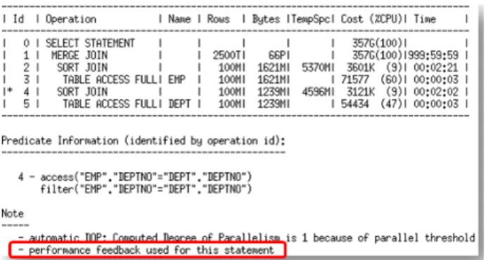
If performance feedback is used for a SQL statement then it is reported in the note section under the plan as shown in figure 14.
NOTE: Even if AutoDOP is not enabled in adaptive mode, statistics feedback may influence the degree of parallelism chosen for a statement.
Figure 14. Execution plan for a SQL statement that was found to run better serial by performance feedback
SQL plan directives
SQL plan directives are automatically created based on information learnt via Automatic
Reoptimization. A SQL plan directive is additional information that the optimizer uses to generate a more optimal execution plan. For example, when joining two tables that have a data skew in their join columns, a SQL plan directive can direct the optimizer to use dynamic statistics to obtain a more accurate join cardinality estimate.
SQL plan directives are created on query expressions rather than at a statement or object level to ensure they can be applied to multiple SQL statements. It is also possible to have multiple SQL plan directives used for a SQL statement. The number of SQL plan directives used for a SQL statement is shown in the note section under the execution plan (Figure 15).
Figure 15. The number of SQL plan directives used for a statement is shown in the note section under the plan The database automatically maintains SQL plan directives, and stores them in the SYSAUX tablespace. Any SQL plan directive that is not used after 53 weeks will be automatically purged. SQL plan directives can also be manually managed using the package DBMS_SPD. However, it is not possible to
manually create a SQL plan directive. SQL plan directives can be monitored using the views
DBA_SQL_PLAN_DIRECTIVES and DBA_SQL_PLAN_DIR_OBJECTS (See Figure 16).
As mentioned above, a SQL plan directive was automatically created for the SQL statement shown in Figure 10 after it was discovered that the optimizer’s cardinality estimates vary greatly from the actual number of rows return by the operations in the plan. In fact, two SQL plan directives were
automatically created. One to correct the cardinality misestimate on the customers table caused by correlation between the multiple single-column predicates and one to correct the cardinality misestimate on the sales table.
Figure 16. Monitoring SQL plan directives automatically created based on information learnt via reoptimization Currently there is only one type of SQL plan directive, ‘DYNAMIC_SAMPLING’. This tells the optimizer that when it sees this particular query expression (for example, filter predicates on country_id,
cust_city, and cust_state_province being used together) it should use dynamic sampling to address the cardinality misestimate.
SQL plan directives are also used by Oracle to determine if extended statistics2, specifically column
groups, are missing and would resolve the cardinality misestimates. After a SQL directive is used the optimizer decides if the cardinality misestimate could be resolved with a column group. If so, it will automatically create that column group the next time statistics are gathered on the appropriate table. The extended statistics will then be used in place of the SQL plan directive when possible (equality predicates, group bys etc.). If the SQL plan directive is no longer necessary it will be automatically purged after 53 weeks.
Take for example, the SQL plan directive 16334867421200019996 created on the customers table in the previous example. This SQL plan directive was created because of the correlation between the multiple single-column predicates used on the customers table. A column group on CUST_CITY,
CUST_STATE_PROVINCE, and COUNTRY_ID columns would address the cardinality misestimate. The next time statistics are gathered on the customers table the column group is automatically created.
Figure 17. Column group automatically created based on SQL plan directive
The next time this SQL statement is executed the column group statistics will be used instead of the SQL plan directive. The state column in DBA_SQL_PLAN_DIRECTIVES indicates where in this cycle a SQL plan directive is currently.
Once the single table cardinality estimates have been address additional SQL plan directives may be created for the same statement to address other problems in the plan like join or group by cardinality misestimates.
Optimizer statistics
Optimizer statistics are a collection of data that describe the database and the objects in it. The optimizer uses these statistics to choose the best execution plan for each SQL statement. Being able to gather the appropriate statistics in a timely manner is critical to maintaining acceptable performance on any Oracle system. With each new release, Oracle strives to provide the necessary statistics
automatically.
New types of histograms
Histograms tell the optimizer about the distribution of data within a column. By default, the optimizer assumes a uniform distribution of rows across the distinct values in a column and will calculate the cardinality for a query with an equality predicate by dividing the total number of rows in the table by the number of distinct values in the column used in the equality predicate. The presence of a histogram changes the formula used by the optimizer to determine the cardinality estimate, and allows it to generate a more accurate estimate. Prior to Oracle Database 12c, there were two types of histograms, frequency and height balance. Two additional types of histogram are now available, namely, top-frequency and hybrid histograms.
Top-Frequency histograms
Traditionally, if a column had more than 254 distinct values and the number of buckets specified is AUTO a height-balanced histogram would be created. But what if 99% or more of the rows in the table had less than 254 distinct values? If a height-balance histogram is created, it runs the risk of not capturing all of the popular values in the table as the endpoint of multiple buckets. Thus some popular values will be treated as non-popular values, which could result in a sub-optimal execution plan being chosen.
In this scenario, it would be better to create a frequency histogram on the extremely popular values that make up the majority of rows in the table and to ignore the unpopular values, in order to create a better quality histogram. This is the exact approach taken with top-frequency histograms. A frequency histogram is created on the most popular values in the column, when those values appear in 99% or more of the rows in the table. This allows all of the popular values in the column to be treated as such. A top-frequency histogram is only created if the ESTIMATE_PERCENT parameter of the gather statistics command is set to AUTO_SAMPLE_SIZE, as all values in the column must be seen in order to
determine if the necessary criteria are met (99.6% of rows have 254 or less distinct values). Take for example the PRODUCT_SALES table, which contains sales information for a Christmas ornaments company. The table has 1.78 million rows and 632 distinct TIME_IDs. But the majority of the rows in PRODUCT_SALES have less than 254 distinct TIME_IDs, as the majority of Christmas ornaments are sold in December each year. A histogram is necessary on the TIME_ID column to make the Optimizer aware of the data skew in the column. In this case a top-frequency histogram is created containing 254 buckets.
Figure 19. Data distribution of TIME_ID column in PRODUCT_SALES table & top-frequency histogram that is created on it
Hybrid histograms
In previous releases, a height balanced histogram was created when the number of distinct values in a column was greater than 254. Only values that appear as the end point of two or more buckets of a height balanced histogram are considered popular. One prominent problem with height balanced histograms is that a value with a frequency that falls into the range of 1/254 of the total population and 2/254 of the total population may or may not appear as a popular value. Although it might span across two 2 buckets it may only appear as the end point value of one bucket. Such values are referred to as almost popular values. Height balanced histograms do not differentiate between almost popular values and truly unpopular values.
A hybrid histogram is similar to the traditional height-balanced histogram, as it is created when the number of distinct values in a column is greater than 254. However, that’s where the similarities end. With a hybrid histogram no value will be the endpoint of more than one bucket, thus allowing the histogram to have more endpoint values or effectively more buckets than a height-balanced histogram. So, how does a hybrid histogram indicate a popular value? The frequency of each endpoint value is recorded (in a new column endpoint_repeat_count), thus providing an accurate indication of the popularity of each endpoint value.
Take for example the CUST_CITY_ID column in the CUSTOMERS table. There are 55,500 rows in the
CUSTOMERS table and 620 distinct values in the CUST_CITY_ID column. Neither a frequency nor a top-frequency histogram is an option in this case. In Oracle Database 11g, a height balanced histogram is created on this column. The height balanced histogram has 213 buckets but only represents 42 popular values (value is the endpoint of 2 or more buckets). The actual number of popular values in
CUST_CITY_ID column is 54 (i.e., column values with a frequency that is larger than
num_rows/num_buckets = 55500/254= 54).
In Oracle Database 12c a hybrid histogram is created. The hybrid histogram has 254 buckets and represents all 54 popular values. The hybrid histogram actually treats 63 values as popular values. This means that values that were considered as nearly popular (endpoint value of only 1 bucket) in Oracle Database 11g are now treated as popular values and will have a more accurate cardinality estimate. Figure 20 shows an example of how a nearly popular value (52114) in Oracle Database 11g get a much better cardinality estimate in Oracle Database 12c.
Figure 20. Hybrid histograms achieve more accurate cardinality estimates for what was considered a nearly popular value in Oracle Database 11g
Online statistics gathering
When an index is created, Oracle automatically gathers optimizer statistics as part of the index creation by piggybacking the statistics gather on the full data scan necessary for the index creation. The same technique is now being applied for direct path operations such as, create table as select (CTAS) and insert as select (IAS) operations. Piggybacking the statistics gather as part of the data loading operation, means no additional full data scan is required to have statistics available immediately after the data is loaded.
Figure 21. Online statistic gathering provides both table and column statistics for newly created SALES2 table Online statistics gathering does not gather histograms or index statistics, as these types of statistics require additional data scans, which could have a large impact on the performance of the data load. To gather the necessary histogram and index statistics without re-gathering the base column statistics use the DBMS_STATS.GATHER_TABLE_STATS procedure with the new options parameter set to GATHER AUTO.
The notes column “HISTOGRAM_ONLY” indicates that histograms were gathered without re-gathering basic column statistics. The GATHER AUTO option is only recommended to be used after online statistics gathering has occurred.
There are two ways to confirm online statistics gathering has occurred: check the execution plan to see if the new row source OPTIMIZER STATISTICS GATHERING appears in the plan or look in the new
notes column of the USER_TAB_COL_STATISTICS table for the status STATS_ON_LOAD.
Figure 23. Execution plan for an on-line statistics gathering operation
Since online statistics gathering was designed to have a minimal impact on the performance of a direct path load operation it can only occur when data is being loaded into an empty object. To ensure online statistics gathering kicks in when loading into a new partition of an existing table, use extended syntax to specify the partition explicitly. In this case partition level statistics will be created but global level (table level) statistics will not be updated. If incremental statistics have been enabled on the partitioned table a synopsis will be created as part of the data load operation.
Figure 24. Online statistics gathering kicking in for IAS operation into existing partitioned table
Note, it is possible to disable online statistics gathering at the statement level by specifying the hint
NO_GATHER_OPTIMIZER_STATISTICS.
Session level statistics on Global Temporary Tables
Global temporary tables are often used to store intermediate results in an application context. A global temporary table shares (GTT) its definition system-wide with all users with the appropriate privileges, but the data content is always session-private. It has always been possible to gather statistics on a global temporary table (that persist rows on commit); however in previous releases the statistics gathered would be used by all sessions accessing that table. This was less than ideal if the volume or nature of the data stored in the GTT differed greatly between sessions.
It is now possible to have a separate set of statistics for every session using a GTT. Statistics sharing on a GTT is controlled using a new DBMS_STATS preference GLOBAL_TEMP_TABLE_STATS. By default
the preference is set to SESSION, meaning each session accessing the GTT will have it’s own set of statistics. The optimizer will try to use session statistics first but if session statistics do not exist, then optimizer will use shared statistics. If you want to revert back to the prior behavior of only one set of
statistics used by all session, set the GLOBAL_TEMP_TABLE_STATS preference to SHARED.
Figure 25. Changing the default behavior of not sharing statistics on a GTT to forcing statistics sharing
When populating a GTT (that persists rows on commit) using a direct path operation, session level statistics will be automatically created due to online statistics gathering, which will remove the necessity to run additional statistics gathering command and will not impact the statistics used by any other session.
Figure 26. Populating a GTT using a direct path operation results in session level statistics being automatically gathered
New reporting subprograms in DBMS_STATS package
Knowing when and how to gather statistics in a timely manner is critical to maintain acceptable performance on any system. Determining what statistics gathering operations are currently executing in an environment and how changes to the statistics methodology will impact the system can be difficult and time consuming.
In Oracle Database 12c, new reporting subprograms have been added to the DBMS_STATS package to make it easier to monitor what statistics gathering activities are currently going on and what impact changes to the parameter settings of these operations will have.
REPORT_STATS_OPERATIONS
This new function generates a report that shows detailed information about what statistics gathering operations have occurred, during a specified time window. The report gives details on when each operation occurred, its status, and the number of objects covered. The report can be displayed in either text or HTML format.
Figure 27. Generating a new DBMS_STATS.REPORT_STATS_OPERATIONS report REPORT_SINGLE_STATS_OPERATION
This new function generates a detailed report for a specified statistics gathering operations. REPORT_GATHER_*_STATS
This new set of functions don't actually gather statistics, but reports the list of objects that would be processed if the corresponding GATHER_*_STATS procedure was called with the same parameter settings. The REPORT_GATHER_*_STATS functions take the same input parameters as for the corresponding GATHER_*_STATS procedure and two additional parameters: detail level and format.
New Optimization Techniques
Oracle transforms SQL statements using a variety of sophisticated techniques during query optimization. The purpose of this phase of query optimization is to transform the original SQL statement into a semantically equivalent SQL statement that can be processed more efficiently. In Oracle Database 12c, several new query optimizations were introduced.
Partial Join Evaluation
Partial join evaluation is an optimization technique that is performed during join order generation. The goal of this technique is to avoid generating duplicate rows that would otherwise be removed by a distinct operator later in the plan. By replacing the distinct operator with an inner join or a semi-join earlier in the plan, the number of rows produced by this step will be reduced. This should improve the overall performance of the plan, as subsequent steps will only have to operate on a reduced set of rows. This optimization can be applied to the following types of query block: MAX(), MIN(), SUM (distinct), AVG (distinct), COUNT (distinct), branches of the UNION, MINUS, INTERSECT operators, [NOT] EXISTS sub queries, etc.
Consider the following DISTINCT query,
In Oracle Database 11g, the join between ORDERS and CUSTOMERS is a hash join that must be fully
evaluated before a unique sort is done to eliminate any duplicate rows.
Figure 29. Oracle database 11g plan requires complete join between ORDERS & CUSTOMERS with duplicates removed via a unique sort
With partial join evaluation, the join between ORDERS and CUSTOMERS is converted to a semi-join, which means as soon as one match is found for a CUSTOMER_ID in the CUSTOMERS table the query moves on to the next CUSTOMER_ID. By converting the hash join to a semi-join, the number of rows flowing into the SORT UNIQUE is greatly reduced because the duplicates have already been eliminated. The plan for the transformed SQL is shown in Figure 30.
Figure 30. Oracle database 12c plan shows semi join between ORDERS & CUSTOMERS resulting in no duplicates being generated.
Null accepting semi-joins
It is not uncommon for application developers to add an IS NULL predicate to a SQL statement that contains an EXISTS subquery. The additional IS NULL predicate is added because the semi join resulting from the EXISTS subquery removes rows that have null values, just like an inner join would. Consider the following query,
The assumption here is that the column s.cust_id may have null values and we want to return those rows. Prior to Oracle Database12c the EXISTS subquery cannot be unnested because it appears in an OR predicate (disjunction) with the IS NULL predicate. Not being able to unnest the subquery results in a suboptimal plan where the subquery is applied as a filter after the join between the SALES and
PRODUCTS table.
Figure 31. Oracle database 11g plan shows the EXISTS subquery being applied as a filter after the join.
In Oracle Database 12c a new type of semi-join has been introduced, called a null-accepting semi-join. This new join extends the semi-join algorithm to check for null values in join column of the table on the left hand side of the join. In this case that check would be done on s.cust_id. If the column does contain a null value, then the corresponding row from the SALES table is returned, else the semi-join is performed to determine if the row satisfies the join condition. The null-accepting semi-join plan is shown in figure 32 below.
Figure 32. Oracle database 12c plan shows the EXISTS subquery has been unnested and a null-accepting semi-join is used between customers and sales.
Scalar Subquery Unnesting
A scalar subquery is a subquery that appears in the SELECT clause of a SQL statement. Scalar
subqueries are not unnested, so a correlated scalar subquery (one that references a column outside the subquery) needs to be evaluated for each row produced by the outer query. Consider the following query,
In Oracle Database 11g, for each row in the CUSTOMERS table where the CUST_CREDIT_LIMIT is greater than 50,000 the scalar subquery on the SALES table must be executed. The SALES table is large and scanning it multiple times is very resource intensive.
Figure 33. Oracle database 11g plan shows the scalar subquery has to be evaluated for every row returned from customers table.
Unnesting the scalar subquery and converting it into a join would remove the necessity of having to evaluate it for every row in the outer query. In Oracle Database 12c scalar subqueries can be unnested and in this example the scalar subquery on the SALES table is converted into a group-by view. The group-by view is guaranteed to return a single row, just as the subquery was. An outer join is also added to the query to ensure a row from the CUSTOMERS table will be returned even if the result of the view is NULL. The transformed query will be as follows,
Figure 34. Oracle database 12c plan shows the scalar subquery has been unnested with the use of an outer join and group view.
Multi-Table Left Outer Join
Prior to Oracle Database12c, having multiple tables on the left of an outer join was illegal and resulted in an ORA-01417 error.
The only way to execute such a query was to translate it into ANSI syntax. However, the
implementation of such ANSI syntax results in a lateral view3 being used. Oracle is unable to merge a
lateral view, so the Optimizer’s plan choices are limited in terms of join order and join method, which may result in a sub-optimal plan.
Figure 36. ANSI syntax results in a plan with a lateral view, which cannot be merged, thus limiting the join order In Oracle Database 12c, multi-table left outer join specified in Oracle syntax (+) are now supported. It is also possible to merge multi-table views on the left hand side of an outer-join. The ability to merge the views enables more join orders and join methods to be considered, resulting in a more optimal plan being selected.
Figure 37. New multi-table left outer join support allows view merging and results in a more optimal plan
Initialization parameters
There are several new initialization parameters that govern the optimizer and its new features in Oracle Database 12c. Below are the details on the new parameters.
OPTIMIZER_ADAPTIVE_FEATURES
The use of the new adaptive query optimization functionality, including adaptive joins and the creation and use of SQL plan directives, is controlled by the OPTIMIZER_ADAPTIVE_FEATURES parameter. The default value for this parameter is tied to the value of OPTIMIZER_FEATURES_ENABLE (OFE). If OFE is set to 12.1.0.1 or higher, then OPTIMIZER_ADAPTIVE_FEATURES is set to TRUE and all of the adaptive query optimization features will be used. If OFE is set to a value lower than 12.1.0.1 then
OPTIMIZER_ADAPTIVE_FEATURES will be set to false and none of the adaptive query optimization features will be used.
OPTIMIZER_ADAPTIVE_REPORTING_ONLY
The prospect of an execution plan adapting or change mid-execution may seem frightening at first. In order to get a better understand of how many SQL statements will be affect by the new adaptive plans, it is possible to enable adaptive plan in a reporting mode only by setting
OPTIMIZER_ADAPTIVE_REPORTING_ONLY to TRUE (default is FALSE). In this mode, information needed to enable adaptive join methods is gathered, but no action is taken to change the plan. This means the default plan will always be used but information is collected on how the plan would have adapted in non-reporting mode.
OPTIMIZER_DYNAMIC_SAMPLING
Although the parameter OPTIMIZER_DYNAMIC_SAMPLING is not new, it does have a new level, 11 that controls the creation of dynamic statistics. When set to level 11 the Optimizer will automatically determine which statements would benefit from dynamic statistics, even if all of the objects have statistics.
Enhancements to existing functionality
During the development of Oracle Database 12c a lot of time was also devoted to improving existing optimizer features and functionality to make it easier to have the best possible statistics available and to ensure the most optimal execution plan is always chosen. This section describes in details the
enhancements made to the existing aspect of the optimizer and the statistics that feed it. SQL Plan Management
SQL plan management (SPM) was one of the most popular optimizer new features in Oracle Database 11g as it ensures that runtime performance will never degrade due to the change of an execution plan. To guarantee this, only accepted execution plans are used; any plan evolution that does occur, is tracked and evaluated at a later point in time, and only accepted if the new plan shows a noticeable improvement in runtime. SQL Plan Management has three main components:
1. Plan capture:
Creation of SQL plan baselines that store accepted execution plans for all relevant SQL statements. SQL plan baselines are stored in the SQL Management Base in the SYSAUX tablespace.
2. Plan selection:
Ensures only accepted execution plans are used for statements with a SQL plan baseline and records any new execution plans found for a statement as unaccepted plans in the SQL plan baseline.
3. Plan evolution:
Evaluate all unaccepted execution plans for a given statement, with only plans that show a performance improvement becoming accepted plans in the SQL plan baseline.
In oracle Database 12c, the plan evolution aspect of SPM has been enhanced to allow for automatic plan evolution.
Automatic plan evolution is done by the SPM evolve advisor. The evolve advisor is an AutoTask
(SYS_AUTO_SPM_EVOLVE_TASK), which operates during the nightly maintenance window and automatically runs the evolve process for accepted plans in SPM. The AutoTask ranks all non-accepted plan in SPM (newly found plans ranking highest) and then run the evolve process for as many plans as possible before the maintenance window closes.
All of the non-accepted plans that perform better than the existing accepted plan in their SQL plan baseline are automatically accepted. However, any non-accepted plans that fail to meet the
performance criteria remain unaccepted and their LAST_VERIFIED attribute will be updated with the current timestamp. The AutoTask will not attempt to evolve an unaccepted plan again for at least another 30 days and only then if the SQL statement is active (LAST_EXECUTED attribute has been updated).
The results of the nightly evolve task can be viewed using the
DBMS_SPM.REPORT_AUTO_EVOLVE_TASK function. All aspects of the SPM evolve advisor can be
managed via Enterprise Manager or the DBMS_AUTO_TASK_ADMIN PL/SQL package.
Alternatively, it is possible to evolve an unaccepted plan manually using Oracle Enterprise Manager or the supplied package DBMS_SPM. From Oracle Database 12c onwards, the original SPM evolve function (DBMS_SPM.EVOLVE_SQL_PLAN_BASELINE) has been deprecated in favor of a new API that calls the evolve advisor. Figure 38, shows the sequence of steps needs to invoke the evolve advisor. It is
typically a three step processes beginning with the creation of an evolve task. Each task is given a unique name, which enables it to be executed multiple times. Once the task has been executed you can review the evolve report by supplying the TASK_ID and EXEC_ID to the
DBMS_SPM.REPORT_EVOLVE_TASK function.
Figure 38. Necessary steps required to manually invoke the evolve advisor
When the evolve advisor is manually invoked the unaccepted plan(s) is not automatically accepted even if it meets the performance criteria. The plans must be manually accepted using the
DBMS_SPM.ACCEPT_SQL_PLAN_BASELINE procedure. The evolve report contains detailed instructions, including the specific syntax, for accept the plan(s).
Originally only the outline (complete set of hints needed to reproduce a specific plan) for a SQL statement was captured as part of a SQL plan baseline. From Oracle Database 12c onwards the actual execution plan will also be recorded when a plan is added to a SQL plan baseline. For plans that were added to a SQL plan baseline in previous releases the actual execution will be added to the SQL plan baseline the first time it’s executed in Oracle Database 12c.
It’s important to capture the actual execution plans to ensure if a SQL plan baseline is moved from one system to another, the plans in the SQL plan baseline can still be displayed even if some of the objects used in it or the parsing schema itself does not exist on the new system. Note that displaying a plan from a SQL plan baseline is not the same as being able to reproduce a plan.
The detailed execution plan for any plan in a SQL plan baseline can be displayed by clicking on the plan name on the SQL plan baseline page in Enterprise Manager or use the procedure
DBMS_XPLAN.DISPLAY_SQL_PLAN_BASELINE. Figure 40, shows the execution plan for the accepted plan (SQL_PLAN_6zsnd8f6zsd9g54bc8843). The plan shown, is the actual plan that was captured
when this plan was added to the SQL plan baseline because the attribute ‘plan rows’ is set to ‘From dictionary’. For plays displayed based on an outline, the attribute ‘plan rows’ is set to ‘From outline’.
Statistics enhancements
Along with the many new features in the area of optimizer statistics, several enhancements were made to existing statistics gathering techniques.
Incremental Statistics
Gathering statistics on partitioned tables consists of gathering statistics at both the table level (global statistics) and (sub) partition level. If the INCREMENTAL preference for a partitioned table is set to
TRUE, the DBMS_STATS.GATHER_*_STATS parameter GRANULARITY includes GLOBAL, and
ESTIMATE_PERCENT is set to AUTO_SAMPLE_SIZE, Oracle will accurately derive all global level statistics by aggregating the partition level statistics.
Incremental global statistics works by storing a synopsis for each partition in the table. A synopsis is statistical metadata for that partition and the columns in the partition. Aggregating the partition level statistics and the synopses from each partition will accurately generate global level statistics, thus eliminating the need to scan the entire table.
Incremental statistics and staleness
In Oracle Database 11g, if incremental statistics were enabled on a table and a single row changed in one of the partitions, then statistics for that partition were considered stale and had to be re-gathered before they could be used to generate global level statistics.
In Oracle Database 12c a new preference called INCREMENTAL_STALENESS allows you to control when partition statistics will be considered stale and not good enough to generate global level statistics. By default, INCREMENTAL_STALENESS is set to NULL, which means partition level statistics are considered stale as soon as a single row changes (same as 11g).
Alternatively, it can be set to USE_STALE_PERCENT or USE_LOCKED_STATS. USE_STALE_PERCENT
means the partition level statistics will be used as long as the percentage of rows changed is less than the value of the preference STALE_PRECENTAGE (10% by default). USE_LOCKED_STATS means if statistics on a partition are locked, they will be used to generate global level statistics regardless of how many rows have changed in that partition since statistics were last gathered.
Incremental statistics and partition exchange loads
One of the benefits of partitioning is the ability to load data quickly and easily, with minimal impact on the business users, by using the exchange partition command. The exchange partition command allows the data in a non-partitioned table to be swapped into a specified partition in the partitioned table. The command does not physically move data; instead it updates the data dictionary to exchange a pointer from the partition to the table and vice versa.
In previous releases, it was not possible to generate the necessary statistics on the non-partitioned table to support incremental statistics during the partition exchange operation. Instead statistics had to be gathered on the partition after the exchange had taken place, in order to ensure the global statistics could be maintained incrementally.
In Oracle Database 12c, the necessary statistics (synopsis) can be created on the non-partitioned table so that, statistics exchanged during a partition exchange load can automatically be used to maintain incrementally global statistics. The new DBMS_STATS table preference INCREMENTAL_LEVEL can be used to identify a non-partitioned table that will be used in partition exchange load. By setting the
INCREMENTAL_LEVEL to TABLE (default is PARTITION), Oracle will automatically create a synopsis for
the table when statistics are gathered. This table level synopsis will then become the partition level synopsis after the load the exchange.
Concurrent Statistics
In Oracle Database 11.2.0.2, concurrent statistics gathering was introduced. When the global statistics gathering preference CONCURRENT is set, Oracle employs the Oracle Job Scheduler and Advanced Queuing components to create and manage one statistics gathering job per object (tables and / or partitions) concurrently.
In Oracle Database 12c, concurrent statistics gathering has been enhanced to make better use of each scheduler job. If a table, partition, or sub-partition is very small or empty, the database may
automatically batch the object with other small objects into a single job to reduce the overhead of job maintenance.
Concurrent statistics gathering can now be employed by the nightly statistics gathering job by setting the preference CONCURRENT is to ALL or AUTOMATIC. The new ORA$AUTOTASK consumer group has been added to the Resource Manager plan active used during the maintenance window, to ensure concurrent statistics gathering does not use to much of the system resources.
Automatic column group detection
Extended statistics help the Optimizer improve the accuracy of cardinality estimates for SQL statements that contain predicates involving a function wrapped column (e.g. UPPER(LastName)) or multiple columns from the same table used in filter predicates, join conditions, or group-by keys. Although extended statistics are extremely useful it can be difficult it know which extended statistics should be created if you are not familiar with an application or data set.
Auto Column Group detection, automatically determines which column groups are required for a table based on a given workload. Please note this functionality does not create extended statistics for function wrapped columns it is only for column groups. Auto Column Group detection is a simple three step process:
1. Seed column usage
Oracle must observe a representative workload, in order to determine the appropriate column groups. The workload can be provided in a SQL Tuning Set or by monitoring a running system. The new procedure DBMS_STATS.SEED_COL_USAGE, should be used it indicate the workload and to tell Oracle how long it should observe that workload. The following example turns on monitoring for 5 minutes or 300 seconds for the current system.
Figure 41. Enabling automatic column group detection
The monitoring procedure records different information from the traditional column usage information you see in sys.col_usage$ and stores it in sys.col_group_usage$. Information is stored for any SQL statement that is executed or explained during the monitoring window. Once the monitoring window has finished, it is possible to review the column usage information recorded for a specific table using the new function
DBMS_STATS.REPORT_COL_USAGE. This function generates a report, which lists what columns from the table were seen in filter predicates, join predicates and group by clauses in the workload. It is also possible to view a report for all the tables in a specific schema by running DBMS_STATS.REPORT_COL_USAGE and providing just the schema name and NULL
for the table name.
Figure 42. Enabling automatic column group detection
2. Create the column groups
Calling the DBMS_STATS.CREATE_EXTENDED_STATS function for each table, will
automatically create the necessary column groups based on the usage information captured during the monitoring window. Once the extended statistics have been created, they will be automatically maintained whenever statistics are gathered on the table.
Alternatively the column groups can be manually creating by specifying the group as the third argument in the DBMS_STATS.CREATE_EXTENDED_STATS function.
Figure 43. Create the automatically detected column groups
3. Regather statistics
groups will have statistics created for them.
Figure 44. Column group statistics are automatically maintained every time statistics are gathered
Conclusion
The optimizer is considered one of the most fascinating components of the Oracle Database because of its complexity. Its purpose is to determine the most efficient execution plan for each SQL statement. It makes these decisions based on the structure of the query, the available statistical information it has about the data, and all the relevant optimizer and execution features.
In Oracle Database 12c the optimizer takes a giant leap forward with the introduction of a new adaptive approach to query optimizations and the enhancements made to the statistical information available to it.
The new adaptive approach to query optimization enables the optimizer to make run-time adjustments to execution plans and to discover additional information that can lead to better statistics. Leveraging this information in conjunction with the existing statistics should make the optimizer more aware of the environment and allow it to select an optimal execution plan every time.
As always, we hope that by outlining in detail the changes made to the optimizer and statistics in this release, the mystery that surrounds them has been removed and this knowledge will help make the upgrade process smoother for you, as being forewarned is being forearmed!
White Paper Title June 2013 Author: Maria Colgan
Oracle Corporation World Headquarters 500 Oracle Parkway Redwood Shores, CA 94065 U.S.A.
Worldwide Inquiries: Phone: +1.650.506.7000 Fax: +1.650.506.7200
oracle.com
Copyright © 2012, Oracle and/or its affiliates. All rights reserved. This document is provided for information purposes only and the contents hereof are subject to change without notice. This document is not warranted to be error-free, nor subject to any other warranties or conditions, whether expressed orally or implied in law, including implied warranties and conditions of merchantability or fitness for a particular purpose. We specifically disclaim any liability with respect to this document and no contractual obligations are formed either directly or indirectly by this document. This document may not be reproduced or transmitted in any form or by any means, electronic or mechanical, for any purpose, without our prior written permission.
Oracle and Java are registered trademarks of Oracle and/or its affiliates. Other names may be trademarks of their respective owners.
Intel and Intel Xeon are trademarks or registered trademarks of Intel Corporation. All SPARC trademarks are used under license and are trademarks or registered trademarks of SPARC International, Inc. AMD, Opteron, the AMD logo, and the AMD Opteron logo are trademarks or registered trademarks of Advanced Micro Devices. UNIX is a registered trademark of The Open Group. 0612