Abstract—Workforce management is a critical component of call center operations. Since labor costs are a major component of the total cost of operation efficient staff scheduling is critical. But because of uncertainty in arrival rates, efficient scheduling is very difficult. While there are many models in the literature that address call center scheduling, the majority of these models ignore the issue of arrival rate uncertainty and focus only on the stochastic variability of interarrival times given a known arrival rate. In this paper I summarize my research into the issue of arrival rate uncertainty and its impact on scheduling. I review empirical data from outsourced call centers that demonstrates the level of uncertainty present in many applications, and propose scheduling and staffing models that consider arrival rate uncertainty.
Index Terms—Call Centers, Stochastic Optimization, Uncertainty, Workforce Management
I. INTRODUCTION
all centers are a large and growing component of the U.S. and world economy. In 1999 an estimated 1.5 million workers were employed in call centers in the US alone[1]. Call center applications include telemarketing, customer service, help desk support, and emergency dispatch. Large scale call centers are technically and managerially sophisticated operations and have been the subject of substantial academic research.
Since labor costs often account for up to 60-70% of the cost of operating a call center [1], efficient staff scheduling is critical. However, the uncertainty associated with key factors such as arrival rates or agent productivity make efficient scheduling very difficult. This problem is especially acute for call centers subject to strict service level agreements (SLAs) that require the call center to meet some predefined performance metric.
This paper provides a summary of my research into the impact of uncertainty on call center capacity management. For this project I investigate how uncertainty impacts capacity decisions when the call center is obligated to achieve an SLA,
Manuscript received April 15, 2007.
T.R. Robbins is with the Pennsylvania State University, Smeal College of Business, University Park PA 16802 USA (phone: 814-883-0749; e-mail: trrobbins@ psu.edu).
but seeks to do so at a minimal cost. In section II I summarize my empirical analysis of call center data. In section III I discuss standard models commonly used for call center scheduling, and in section IV I present an alternative model. Section V summarizes a hedging strategy based on partial cross training of resources. Section VI provides a summary and outlines ongoing research.
II. ARRIVAL RATE UNCERTAINTY
A. Weekly Variability
Most call centers face non-stationary, seasonal arrival patterns and in many cases aggregate call volume is highly variable. An empirical analysis of call volume data is published in [2]. For my research I analyzed call volumes supplied by a provider of outsourced IT support services. This operation involves providing help desk support to large corporate and government entities globally. While the scope of services varies from account to account, many accounts are 24 x 7 support and virtually all accounts are subject to some form of Service Level Agreement (SLA). There are multiple types of SLAs, but the most common specifies a minimum level of the Telephone Service Factor (TSF). A TSF SLA specifies the proportion of calls that must be answered within a specified time. For example, an 80/120 SLA specifies that 80% of calls must be answered within 120 seconds. A very important point is that the service level applies to an extended period, typically a month. The SLA does not define requirements for a day or an hour. The desk is typically staffed so that at some time the service level is underachieved, sometimes overachieved, and is on target for the entire month. The following table summarizes weekly aggregate call volume from 11 different companies.
Addressing Arrival Rate Uncertainty in Call
Center Workforce Management
Thomas R. Robbins – Penn State University
TABLEI
VARIABILITY OF WEEKLY CALL VOLUME
Average Weekly Volume Std. Dev. of Volume Coefficient of Variation Project 1 248.1 81.7 0.330 Project 2 291.9 92.7 0.318 Project 3 516.7 283.2 0.548 Project 4 560.7 175.0 0.312 Project 5 1,442.9 460.2 0.319 Project 6 1,545.0 504.1 0.326 Project 7 2,599.3 809.5 0.311 Project 8 3,336.9 986.7 0.296 Project 9 4,386.8 1,664.4 0.379 Project 10 7,566.9 3,493.9 0.462 Project 11 8,221.9 1,586.9 0.193
This table shows that volume varies considerably from week to week. It also shows a large variation from project to project, with coefficients of variation of weekly volume as low as .193 and as high as .548.
B. Weekly Seasonality
Call volumes exhibit a strong seasonality pattern over the course of a week. In the following figure we see daily call volume for a typical project shown over a 3 month period.
Calls Offered Daily
0 100 200 300 400 500 600 700 800 900 4/1 4/6 4/11 4/16 4/21 4/26 5/1 5/6 5/11 5/16 5/21 5/26 5/31 6/5 6/10 6/15 6/20 6/25 6/30 Calls_Offered-Daily 7 per. Mov. Avg. (Calls_Offered-Daily)
Fig. 1. Sample Daily Call Volume. This graph illustrates the day to day variability of call volume including large volume spikes.
This graph shows strong “seasonal” variation over the course of a week. Monday’s tend to be the highest volume days with volumes dropping off over the course of the week. Volume on Saturdays is a small fraction of the weekday volume and this particular desk is closed on Sunday. The graph also reveals significant stochastic variability. Tuesdays are, for example, often higher volume than Wednesdays but this is not always the case. During the weeks of 4/26 and 5/16 we see larger volumes on Wednesday than Tuesday. We also see the issue of unanticipated spikes in demand, often referred to as
significant events. This is an extremely common event in support desk operations. A downed server, for example, will generate a large call volume. While some contracts provide SLA relief in the case of significant events, in general the desk must meet the SLA even when significant events occur. The large volume of calls during a significant event not only result
in poor performance, but also create a large proportion of the total calls making it more difficult to achieve a specific percentage of “within SLA” calls.
The following chart summarizes the problem of daily volume variability. The average (M-F) daily call volume for each project is listed along with summary statistics for the daily Forecast vs. Actual (FVA) measure, the ratio actual call volume to forecasted call volume.
TABLEII
FORECASTED VS.ACTUAL CALL VOLUME
The table reveals the challenge related to accurately forecasting volume. Most projects systematically underestimate volume. The standard deviation of the forecast error is large and the range of observed values substantial. It is also worth noting that in general smaller (mid-market) projects are more difficult to forecast than larger projects.
C. Intraday Variability
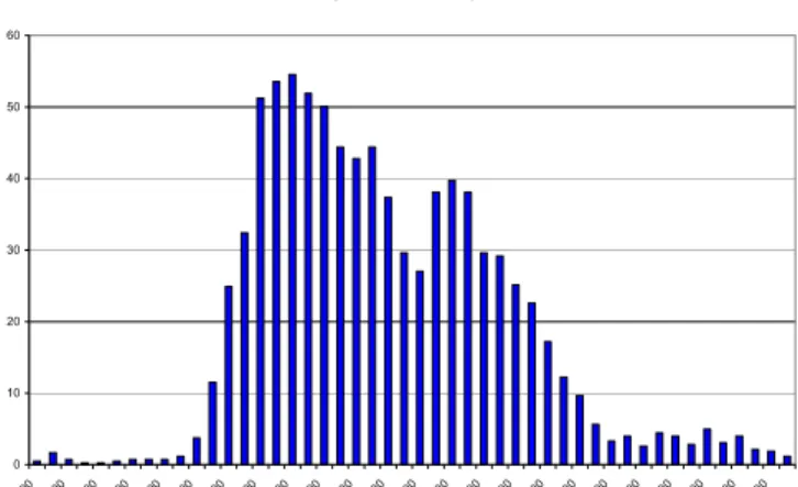
In addition to day-of-week seasonality these call centers also experience very significant time-of-day seasonality. The following figure shows the average call volume presented per ½ hour period to a particular corporate help desk.
Average Call Volume - Project J
0 10 20 30 40 50 60 0:00 1:00 2:00 3:00 4:00 5:00 6:00 7:00 8:00 9:00 10:00 11:0 0 12:0 0 13:0 0 14:0 0 15:0 0 16:0 0 17:0 0 18:0 0 19:0 0 20:0 0 21:0 0 22:0023:0 0
Fig. 2. Sample Average Daily Arrival Pattern. This graph illustrates the daily seasonality of call volume.
This particular desk operates 24x7 and we see that the volume during the overnight hours is quite low. Volume ramps up sharply in the morning with a major surge of calls between 7 and 11 AM. Volume tends to dip down around the lunch break, but a second peak occurs in the afternoon; though the
Forecast vs. Actual
Project Vol/DayAvg. Mean FVA Std Dev of FVA Max of FVA Min of FVA
Project 1 55.2 126.6% 47.7% 334.2% 57.8% Project 2 62.9 130.3% 40.7% 224.4% 56.5% Project 3 100.8 104.7% 41.5% 268.1% 47.4% Project 4 114.6 110.4% 48.1% 407.5% 37.5% Project 5 284.5 91.0% 25.4% 256.5% 64.5% Project 6 313.3 123.4% 24.3% 213.9% 12.9% Project 7 539.1 105.3% 14.3% 152.0% 78.5% Project 8 725.5 96.6% 10.9% 120.1% 51.5% Project 9 873.8 143.4% 38.7% 279.4% 85.5% Project 10 1,417.2 140.4% 26.7% 235.5% 88.2% Project 11 1,714.9 111.1% 25.6% 187.7% 78.0%
afternoon peak is typically lower volume than the morning peak.
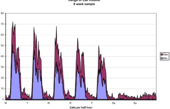
While this basic arrival pattern exists on most business days, there is significant stochastic variability in the call pattern from day to day. The following graph shows call volume over an 8 week period for a particular project. The inner region represents the minimum volume presented in each period, while the overall envelope is the maximum volume presented in each period. The outer region then represents the variability over this eight week period.
Fig. 3. Range of call volume. This graph illustrates the degree to which volume varies from week to week.
This graph shows that while there is significant variability in call volume, a strong seasonal pattern exists.
D. Abandonment
Abandonment rates in this environment also tend to be nonnegligible. The following graph illustrates the daily abandonment rate, along with a 7 day moving average, for a relatively stable project over a 3 ½ year period.
Fig. 4. Abandonment Rate. This graph illustrates that abandonment is a significant and variable factor.
The abandonment rate tends to be in 5% to 10% range and often spikes considerably higher. Most other projects exhibit similar patterns although they tend to have higher average abandonment rates. This shows that any model that ignores abandonment has the potential to introduce significant error.
III. STANDARD SCHEDULING APPROACH
While observed arrival rates are nonstationary and uncertain and abandonment is common, standard queuing models are based on steady state performance with known arrival rates and no abandonment. A widely applied method is the Stationary Independent Period by Period (SIPP) approach [3] that assumes a steady state Erlang C model in each 30 or 60 minute period of the day. “Common practice uses the M/M/N (Erlang C) queuing model to estimate the stationary system performance of short – half hour or hour – interval.” [1] p.92. Furthermore, standard industry practice is to make staffing decisions based on a period by period (local) service level requirement; “each half hour interval’s forecasted λi and µi
give rise to a target staffing level for the period. ... determination of optimal set of schedules can then be described as the solution to an integer program” [1] p.93. Standard models also tend to ignore the uncertainty associated with arrival rates; an issue recognized in literature. “Surprisingly, however, there is little work devoted to an exploration of how [to accommodate uncertainty]” [1] and “What is needed for adequate call center staffing are models that contain both the deviations of the actual mean from the forecast as well as the variation inherent in the Poisson process...” [4].
As was implied above, common practice divides the scheduling process into two independent steps; server sizing and staff scheduling. In the server sizing step, queuing models are used to determine the number of agents required to meet a certain performance metric. While many models use the Erlang C model[5], some model utilize the Erlang A model which allows callers who are put on hold to abandon [6, 7]. While some server sizing models account for variability and/or uncertainty [8, 9] server sizing is typically done without regard to schedule constraints. The staff scheduling step calculates the minimal cost schedule that satisfies the exogenously defined staffing requirements, typically via integer programming [10-12]. Scheduling is then a two step process where each step is optimized locally.
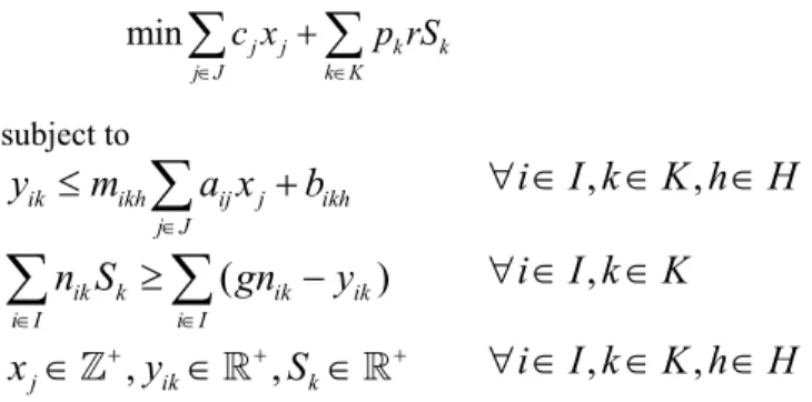
IV. AN INTEGRATED STOCHASTIC SCHEDULING MODEL The standard approach outlined above has three serious shortcomings; it ignores abandonment, it ignores arrival rate uncertainty, and it staffs to a period-by-period SLA. I have developed a scheduling model that address each of these issues; the model integrates the server sizing and staff scheduling steps to achieve a global SLA while allowing for abandonment. The model is formulated as stochastic mixed integer program. The model utilizes a piecewise linear and stationary approximation of the service level curve in each 30 minute period.
To formulate the problem I denote the set of time periods as
I
, the set of feasible schedules asJ
, the set of randomAbandonment Rate 0% 10% 20% 30% 40% 50% 60% 70% 80% 90% 100% Jan-03 Ma r-03 Ma y-0 3 Ju l-03 S ep-03 Nov -03 Jan-04 Ma r-04 Ma y-0 4 Ju l-04 S ep-04 Nov -04 Jan-05 Ma r-05 Ma y-0 5 Ju l-05 S ep-05 Nov -05 Jan-06 Ma r-06 Ma y-0 6 Da ily % of Cal le rs Aba ndoni ng pr ior to s e rv ic e
Abandonment rate 7 per. Mov. Avg. (Abandonment rate)
Range of Call Volume 8 week sample 0 10 20 30 40 50 60 70 80 M T W R F Sa Su
Calls per half hour
Max Min
outcomes of call volume as
K
, and the set of piecewise linear TSF line segments asH
.Given the following definitions:
cj: cost of schedule j
aij: indicates if schedule j is staffed in time i
g: global SLA goal
mikh: slope of piecewise TSF approximation h in period i of
scenario k
bikh: intercept of piecewise TSF approximation h in period i of
scenario k
pk: probability of scenario k
r: per point penalty cost of TSF shortfall
nik: number of calls in period i of scenario k
xj: number of resources assigned to schedule j
yik: number of calls in period i of scenario k answered within
service level
Sk: TSF shortfall in scenario k
A basic formulation of the model can be expressed as:
min j j k k j J k K c x p rS ∈ ∈ +
∑
∑
subject to ik ikh ij j ikh j Jy
m
a x
b
∈≤
∑
+
∀ ∈
i I k K h H
,
∈
,
∈
(
)
ik k ik ik i I i In S
gn
y
∈ ∈≥
−
∑
∑
∀ ∈
i I k K
,
∈
,
,
j ik kx
∈
]
+y
∈
\
+S
∈
\
+∀ ∈
i I k K h H
,
∈
,
∈
I refer to this model as the Stochastic Call Center Scheduling (SCCS) model. In this formulation we generate a series of possible call arrival patterns and optimize over this sample, a standard approach for stochastic programming [13]. The scenarios are generated from a statistical model of arrivals fit to historical call volumes. Although this approach introduces sampling error, standard methods existing for calculating statistical bounds on the expected outcome [14].For each scenario, and each 30 minute time period, we calculate a piece wise linear approximation of the service level curve generated from the Erlang A queuing model. In each period we have h line segments, each of which is characterized by a slope (
m
ikh) and intercept (b
ikh). This piece wise linear model gives the service level that corresponds to the staffing level decision based on the call volume in that thirty minute period. I assume a constant patience factor for all periods and all scenarios.The objective of the optimization program is to minimize the fixed cost of staffing plus the expected cost of not meeting the service level requirement. Staffing costs are based on a standard labor rate and the penalty cost is calculated as a linear function of the percentage shortfall, with a cost of r
dollars per point shortfall. The first inequality calculates the number of calls answered within the service level requirement,
and the second inequality calculates the associated TSF shortfall. The details of the empirical analysis and the scheduling model are presented in [15].
The resulting MIP becomes quite large and is best solved using the L Shaped method, an adaptation of Bender’s decomposition algorithm [13].
I have evaluated this model under a wide range of conditions. Stochastic programs always generate solutions whose expected cost of operation is no greater than models which only consider the expectation of random variables, and is typically much lower; the improvement in expected outcome is known as the Value of the Stochastic Solution [13]. In my testing against models based on several real world projects, I found that VSS ranged from 12% to 21%. I also evaluated this model against the common practice of using Erlang C, period by period constraints and mean value arrival rates. I tested the two models against three arrival patterns with a variety of scheduling options that ranged from five day a week 8 hour shifts only (Sched A) to a variety of full and part time scheduling options (Sched E) for a set of projects with an 80% service level (TSF) target. The results are summarized in the following table
TABLEIII
COMPARING TWO SCHEDULING MODELS
Direct Labor Expected Outcome Average TSF Direct Labor Expected Outcome Average TSF Project J Sched A 16,000 16,000 91.8% 11,280 11,660 81.1% 4,340 27.1% Sched B 13,200 13,200 91.0% 10,800 11,239 80.4% 1,961 14.9% Sched C 12,880 12880 90.4% 10,944 11,235 81.3% 1,645 12.8% Sched D 12,500 12500 89.5% 10,844 11,103 81.5% 1,397 11.2% Sched E 12,300 12300 89.2% 10,720 11,019 81.3% 1,281 10.4% Project S Sched A 38,000 39,565 91.6% 30,960 35,305 83.2% 4,260 10.8% Sched B 32,800 36,647 88.0% 30,320 34,728 83.7% 1,919 5.2% Sched C 32,320 36,504 87.4% 30,384 34,733 83.6% 1,772 4.9% Sched D 30,900 35,720 86.1% 30,092 34,585 83.5% 1,135 3.2% Sched E 30,980 35,776 86.2% 30,096 34,595 83.5% 1,181 3.3% Project O Sched A 13,600 13,984 85.7% 11,600 12,443 80.2% 1,542 11.0% Sched B 12,400 12,914 83.4% 11,360 12,257 80.1% 656 5.1% Sched C 12,160 12,704 83.0% 11,296 12,278 79.5% 426 3.4% Sched D 11,980 12,572 82.4% 11,352 12,210 80.2% 362 2.9% Sched E 11,880 12,504 82.1% 11,316 12,226 79.9% 278 2.2% SCCS - Erlang A Expected Savings
Locally Constrained Erlang C
In all cases the SCCS model provides a lower expected cost of operation than the (mean value) Local Erlang C (LEC) model. The improvement is due to both the recognition of variability, and the integration of the server sizing and staff scheduling steps. In the case of full time shifts (Sched A) the two step process introduces significant excess capacity, driving the average global service level well above the 80% target. In this case expected savings are at least 10% and as high as 27%. But even when staffing is very flexible (Sched E), the SCCS model still lowers costs by improved hedging against variability in arrival patterns.
The fact that the LEC model performs better than the Erlang A mean-value model is quite interesting. The LEC model assumes away abandonment, which leads to over staffing, and
uncertainty, which leads to under staffing. To the extent that these factors cancel out the LEC model can provide reasonable estimates. This suggests that introducing abandonment into staffing models, without also allowing for uncertainty, may not improve results. Overall I find that the SCCS model is quite practical computationally, and leads to lower expected cost of operation.
V. LOWERED COST THROUGH PARTIAL POOLING The stochastic scheduling model described above allows us to better hedge against uncertainty, but does not improve the overall operating characteristics of the queuing system. Further improvement is possible if we develop systems that are more robust to variations in arrival rates or forecasting errors.
In the call centers I studied, agents require extensive training to learn the systems they must support; training that is project specific and quite expensive. As such, agents are typically dedicated to a single project because management feels it is simply too expensive to train agents to support multiple projects. My research focuses on a strategy whereby a relatively small portion of the workforce is cross trained. While base agents remain single project focused, a handful of
super agents are trained to support multiple projects. This is similar to a model developed in [16], except in that model all agents were trained to the same level and the design question was what is the appropriate number of skills to give each agent. In that paper the authors found that most of the benefit accrued by giving the agents two skills, but did not address the cost associated with adding skills. This model differs in that some agents have one skill while some have two, and those agents with two skills are more expensive.
I also find that a little flexibility goes a long way, and most of the benefit of pooling comes from pooling the first few agents. Given that the model associates an incremental cost with cross training, and finds diminishing returns, an optimal level of cross training exists.
The model assumes a simple queuing structure as follows
1 3 2
1 2 Call Types
Feasible Routings
Pools of CSRs
Fig. 5. Basic Queuing Model. The queuing model has two call types and three resource types.
Base agents have priority routing and calls are routed to super agents only when all base agents are busy. When a super comes free they take a call from the largest queue.
My analysis uses discrete event simulation and a neighborhood search algorithm to find near optimal staffing for both steady state and nonstationary (project based) arrival patterns. In the project oriented case we use the SCCS algorithm described above to generate a preliminary schedule. I then use a simulation based optimization search to refine the single project schedule. To find the optimal pooling based schedule I start with the SCCS results and then implement a local search metaheuristic to seek out lower cost pooled schedules. The search is based on a Variable Neighborhood Search methodology, an approach that searches a narrowly defined neighborhood thoroughly, then expands to a larger neighborhood if no improving solution can be found [17]. I investigated the pooling combinations of the three projects evaluated in the previous section, for each of the five possible scheduling options. In this analysis I assume that super agents earn a 25% premium relative to base agents.
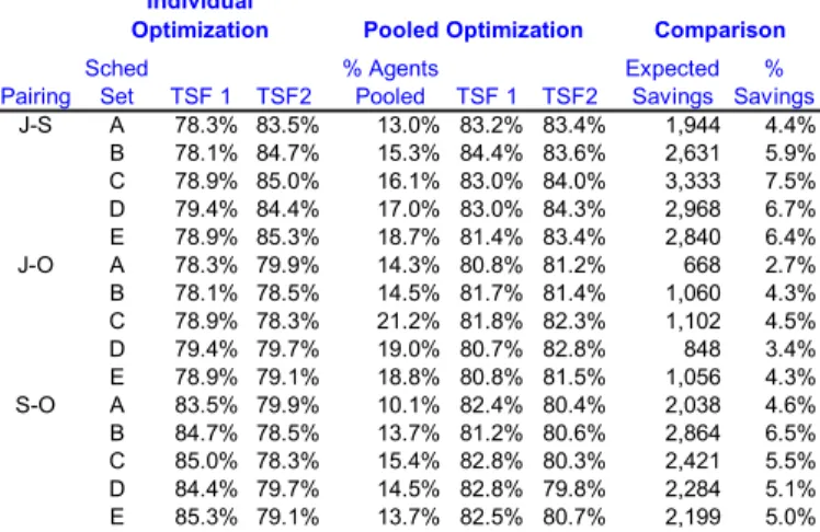
The results of my analysis are summarized in the following table.
TABLEIV
IMPACT OF PARTIAL POOLING ON TOTAL COST OF SERVICE
Pairing Sched Set TSF 1 TSF2 % Agents Pooled TSF 1 TSF2 Expected Savings % Savings J-S A 78.3% 83.5% 13.0% 83.2% 83.4% 1,944 4.4% B 78.1% 84.7% 15.3% 84.4% 83.6% 2,631 5.9% C 78.9% 85.0% 16.1% 83.0% 84.0% 3,333 7.5% D 79.4% 84.4% 17.0% 83.0% 84.3% 2,968 6.7% E 78.9% 85.3% 18.7% 81.4% 83.4% 2,840 6.4% J-O A 78.3% 79.9% 14.3% 80.8% 81.2% 668 2.7% B 78.1% 78.5% 14.5% 81.7% 81.4% 1,060 4.3% C 78.9% 78.3% 21.2% 81.8% 82.3% 1,102 4.5% D 79.4% 79.7% 19.0% 80.7% 82.8% 848 3.4% E 78.9% 79.1% 18.8% 80.8% 81.5% 1,056 4.3% S-O A 83.5% 79.9% 10.1% 82.4% 80.4% 2,038 4.6% B 84.7% 78.5% 13.7% 81.2% 80.6% 2,864 6.5% C 85.0% 78.3% 15.4% 82.8% 80.3% 2,421 5.5% D 84.4% 79.7% 14.5% 82.8% 79.8% 2,284 5.1% E 85.3% 79.1% 13.7% 82.5% 80.7% 2,199 5.0% Individual
Optimization Pooled Optimization Comparison
The data indicates that the introduction of super agents lowers the total cost of operation, even if those super agents earn a 25% premium. I found that cross training only a relatively modest proportion of agents, 10%-21% results in an overall cost savings of 2.7% - 7.5%. Furthermore, we see that the average service level for each project is shifted toward the target level of 80%. The major benefit of this approach is the ability to dynamically reallocate capacity to the project that needs it the most.
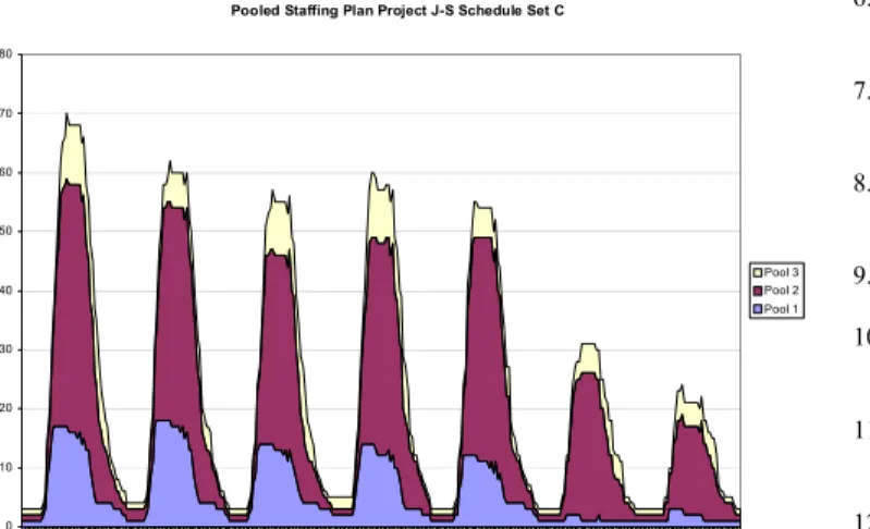
A graphical view of the pooled staffing plan is provided in the following figure. The graph shows that the search algorithm finds that scheduling super agents during busy periods lowers overall operating costs. During these busy periods super agents can be dynamically reallocated to the project with the largest queue.
Pooled Staffing Plan Project J-S Schedule Set C 0 10 20 30 40 50 60 70 80 Pool 3 Pool 2 Pool 1
Fig. 6. Pooled Staffing Model. A group of super agents are available during peak times to dynamically serve the busiest project
VI. CONCLUSION
My research investigates the impact of arrival rate variability on call center operations. Examining data from a number of corporate and government entities reveals that arrival rates exhibit significant variability. The simplifying assumptions of the standard Erlang C model are shown to at least partially cancel and lead to reasonable results, but the stochastic scheduling model always provides better results. In some cases this difference is substantial. I also examine a more complicated queuing system and show that partial cross training lowers costs even when cross training is expensive.
My on-going research is focused on applying these principles to more complicated systems. I am investigating relaxing the assumptions of the Erlang A model to allow for more realistic assumptions, particularly concerning talk time distributions. I am also looking into more complex cross training configuration. In particular I am interested in multi-lingual call centers that may support 10 or more languages with many agents possessing two more language skills.
ACKNOWLEDGMENT
The author would like to thank the various managers at the subject firm that provided access, data, and insight throughout this project.
REFERENCES
1. Gans, N., G. Koole, and A. Mandelbaum, Telephone call centers: Tutorial, review, and research prospects. Manufacturing & Service Operations Management, 2003. 5(2): p. 79-141.
2. Brown, L., et al., Statistical Analysis of a Telephone Call Center: A
Queueing-Science Perspective. Journal of the American Statistical
Association, 2005. 100(469): p. 36-50.
3. Green, L.V., P.J. Kolesar, and J. Soares, Improving the SIPP Approach for Staffing Service Systems That Have Cyclic Demands. Operations Research, 2001. 49(4): p. 549-564.
4. Green, L.V., P. Kolesar, and J. Soares, An Improved Heuristic for Staffing Telephone Call Centers with Limited Operating Hours. Production and Operations Management, 2003. 12(1): p. 46-61. 5. Angus, I., An Introduction to Erlang B and Erlang C.
Telemanagement, 2001. 187(July-August): p. 6-8.
6. Garnett, O., A. Mandelbaum, and M.I. Reiman, Designing a Call Center with impatient customers. Manufacturing & Service Operations Management, 2002. 4(3): p. 208-227.
7. Mandelbaum, A. and S. Zeltyn, Service Engineering in Action: The Palm/Erlang-A Queue, with Applications to Call Centers Draft,
December 2004. 2004.
8. Green, L.V., P.J. Kolesar, and W. Whitt, Coping with Time-Varying Demand when Setting Staffing Requirements for a Service
System. 2005, Columbia University. p. 58.
9. Whitt, W., Staffing a Call Center with Uncertain Arrival Rate and
Absenteeism. Production and Operations Management, 2006.
10. Brusco, M.J. and L.W. Jacobs, Personnel Tour Scheduling When
Starting-Time Restrictions Are Present. Management Science,
1998. 44(4): p. 534-547.
11. Brusco, M.J. and L.W. Jacobs, Optimal Models for Meal-Break and Start-Time Flexibility in Continuous Tour Scheduling. Management Science, 2000. 46(12): p. 1630-1641.
12. Brusco, M.J. and T.R. Johns, A sequential integer programming
method for discontinuous labor tour scheduling. European Journal
of Operational Research, 1996. 95(3): p. 537-548. 13. Birge, J.R. and F. Louveaux, Introduction to Stochastic
Programming. 1997, New York: Springer. xix, 421 p.
14. Mak, W.-K., D.P. Morton, and R.K. Wood, Monte Carlo bounding techniques for determining solution quality in stochastic programs. Operations Research Letters, 1999. 24(1-2): p. 47-56.
15. Robbins, T.R., Managing Service Capacity Under Uncertainty- Unpublished PhD Dissertation
(http://www.personal.psu.edu/faculty/t/r/trr147). 2007,
Pennsylvania State University.
16. Whitt, W., A Staffing Algorithm for Call Centers with Skill-Based
Routing. Manufacturing & Service Operations Management, 2005.
7(4): p. 276-294.
17. Hansen, P. and N. Mladenovic, Variable neighborhood search:
Principles and applications. European Journal of Operational