InferPy Documentation

(1)

Release 1.0

Javier Cózar, Rafael Cabañas, Antonio Salmerón, Andrés R. Masegosa

(2)

(3)

1 Getting Started: 3

2 Guiding Principles 7

3 Requirements 9

4 Guide to Probabilistic Models 11

5 Guide to Approximate Inference 17

6 Guide to Bayesian Deep Learning 21

7 Probabilistic Model Zoo 23

8 inferpy package 31

9 Contact and Support 165

Python Module Index 167

(4)

(5)

InferPy is a high-level API for probabilistic modeling written in Python and capable of running on top of Tensorflow. InferPy’s API is strongly inspired by Keras and it has a focus on enabling flexible data processing, easy-to-code probablistic modeling, scalable inference and robust model validation.

Use InferPy if you need a probabilistic programming language that:

• Allows easy and fast prototyping of hierarchical probabilistic models with a simple and user friendly API in-spired by Keras.

• Automatically creates computational efficient batched models without the need to deal with complex tensor operations.

• Run seamlessly on CPU and GPU by relying on Tensorflow, without having to learn how to use Tensorflow. A set of examples can be found in theProbabilistic Model Zoosection.

(6)

(7)

ONE

GETTING STARTED:

1.1 Installation

Install InferPy from PyPI:

$ python -m pip install inferpy

1.2 30 seconds to InferPy

The core data structures of InferPy is aprobabilistic model, defined as a set ofrandom variableswith a conditional dependency structure. Arandom varibleis an object parameterized by a set of tensors.

Let’s look at a simple non-linearprobabilistic component analysismodel (NLPCA). Graphically the model can be defined as follows,

Fig. 1: Non-linear PCA

We start by importing the required packages and defining the constant parameters in the model. import inferpy as inf

import tensorflow as tf

# number of components k = 1

# size of the hidden layer in the NN d0 = 100

# dimensionality of the data dx = 2

# number of observations (dataset size) N = 1000

(8)

A model can be defined by decorating any function [email protected]. The model is fully specified by the variables defined inside this function:

@inf.probmodel

def nlpca(k, d0, dx, decoder):

with inf.datamodel():

z = inf.Normal(tf.ones([k])_*0.5, 1., name="z") # shape = [N,k] output = decoder(z,d0,dx)

x_loc = output[:,:dx]

x_scale = tf.nn.softmax(output[:,dx:])

x = inf.Normal(x_loc, x_scale, name="x") # shape = [N,d]

The constructwith inf.datamodel(), which resembles to theplateau notation, will replicate N times the variables enclosed, where N is the size of our data.

In the previous model, the input argumentdecodermust be a function implementing a neural network. This might be defined outside the model as follows.

def decoder(z,d0,dx):

h0 = tf.layers.dense(z, d0, tf.nn.relu) return tf.layers.dense(h0, 2 * dx)

Now, we can instantiate our model and obtain samples (from the prior distributions). # create an instance of the model

m = nlpca(k,d0,dx, decoder)

# Sample from priors samples = m.sample()

In variational inference, we must defined a Q-model as follows. @inf.probmodel

def qmodel(k):

qz_loc = inf.Parameter(tf.ones([k])_*0.5, name="qz_loc")

qz_scale = tf.math.softplus(inf.Parameter(tf.ones([k]),name="qz_scale"))

qz = inf.Normal(qz_loc, qz_scale, name="z")

Afterwards, we define the parameters of our inference algorithm and fit the data to the model. # set the inference algorithm

VI = inf.inference.VI(qmodel(k), epochs=5000)

# learn the parameters m.fit({"x": x_train}, VI)

The inference method can be further configure. But, as in Keras, a core principle is to try make things reasonably simple, while allowing the user the full control if needed.

(9)

#extract the hidden representation hidden_encoding = m.posterior["z"]

(10)

(11)

TWO

GUIDING PRINCIPLES

2.1 Features

The main features of InferPy are listed below.

• Allows a simple definition and inference of probabilistic models containing deep neural networks.

• The models that can be defined in InferPy are those that can be defined using Edward2 (i.e.,tfp.edward2, whose probability distribuions are mainly inherited from the module distributions in the tensorflow-probability package.

• Edward’s drawback is that for the model definition, the user has to manage complex multidimensional arrays called tensors. By contrast, in InferPy all the parameters in a model can be defined using the standard Python types (compatibility with Numpy is available as well).

• InferPy directly relies on top of Edward’s inference engine and includes all the inference algorithms included in this package. As Edward’s inference engine relies on TensorFlow computing engine, InferPy also relies on it too.

• Unlike Edward, our package does not require to have a strong background in the inference methods.

2.2 Architecture

Given the previous considerations, we might summarize the InferPy architecture as follows.

Note that InferPy can be seen as an upper layer for working with probabilistic distributions defined over tensors. Most of the interaction is done with Edward: the definitions of the random variables, the inference. However, InferPy also interacts directly with TensorFlow in some operations that are hidden to the user, e.g., the manipulation of the tensors representing the parameters of the distributions.

An additional advantage of using Edward and TensorFlow as inference engine, is that all the paralelisation details are hidden to the user. Moreover, the same code will run either in CPUs or GPUs.

(12)

(13)

THREE

REQUIREMENTS

3.1 System

Currently, InferPy requires Python 3.5 or higher. For checking your default Python version, type: $ python --version

Travis tests are performed on versions 3.5 and 3.6. Go tohttps://www.python.org/for specific instructions for installing the Python interpreter in your system.

InferPy runs in any OS with the Python interpreter installed. In particular, tests have been carried out for the systems listed bellow.

• Linux CentOS 7 • Linux Elementary 0.4 • Linux Mint 19

• Linux Ubuntu 14.04 16.04 18.04

• MacOS High Sierra (10.13) and Mojave (10.14) • Windows 10 Enterprise

3.2 Package Dependencies

For a basic usage, InferPy requires the following packages: tensorflow>=1.12.1,<2.0 tensorflow-probability>=0.5.0,<1.0 networkx>=2.2.0<3.0 matplotlib>=2.2.3,<3.0 Keras==2.2.4 Keras-Applications==1.0.7 Keras-Preprocessing==1.0.9 protobuf==3.8.0

(14)

(15)

FOUR

GUIDE TO PROBABILISTIC MODELS

4.1 Getting Started with Probabilistic Models

InferPy focuses onhierarchical probabilistic modelsstructured in two different layers:

• Aprior modeldefining a joint distribution𝑝(w)over the global parameters of the model. wcan be a single random variable or a bunch of random variables with any given dependency structure.

• Adata or observation modeldefining a joint conditional distribution𝑝(x,z|w)over the observed quantitiesx and the the local hidden variableszgoverning the observationx. This data model is specified in a single-sample basis. There are many models of interest without local hidden variables, in that case, we simply specify the conditional𝑝(x|w). Similarly, eitherxorzcan be a single random variable or a bunch of random variables with any given dependency structure.

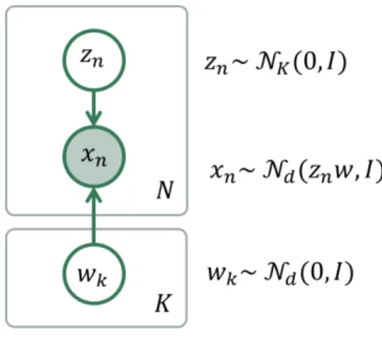
For example, a Bayesian PCA model has the following graphical structure,

Fig. 1: Bayesian PCA

Theprior modelare the variables𝑤𝑘. Thedata modelis the part of the model surrounded by the box indexed byN. And this is how this Bayesian PCA model is denfined in InferPy:

# definition of a generic model @inf.probmodel

def pca(k,d):

w = inf.Normal(loc=np.zeros([k,d]), scale=1, name="w") # shape = [k,d] with inf.datamodel():

z = inf.Normal(np.ones(k),1, name="z") # shape = [N,k] x = inf.Normal(z @ w , 1, name="x") # shape = [N,d]

(16)

(continued from previous page)

# create an instance of the model m = pca(k=1,d=2)

Thewith inf.datamodel()sintaxis is used to replicate the random variables contained within this construct. It follows from the so-called plateau notation to define the data generation part of a probabilistic model. Every replicated variable isconditionally idependentgiven the previous random variables (if any) defined outside thewith statement. The plateau size will be later automatically calculated, so there is not need to specify it. Yet, this construct has an optional input parameter for specifying its size, e.g., with inf.datamodel(size=N). This should be consistent with the size of our data.

4.2 Random Variables

Any random variable in InferPy encapsulates an equivalent one in Edward 2, and hence it also has associated a dis-tribution object from TensorFlow Probability. These can be accessed using the propertiesvaranddistribution

respectively:

>>> x = inf.Normal(loc = 0, scale = 1)

>>> x.var

<ed.RandomVariable 'randvar_0/' shape=() dtype=float32>

>>> x.distribution

<tfp.distributions.Normal 'randvar_0/' batch_shape=() event_shape=() dtype=float32>

Even more, InferPy random variables inherit all the properties and methods from Edward2 variables or TensorFlow Probability distributions (in this order or priority). For example:

>>> x.value

<tf.Tensor 'randvar_0/sample/Reshape:0' shape=() dtype=float32>

>>> x.sample()

-0.05060442

>>> x.loc

<tf.Tensor 'randvar_0/Identity:0' shape=() dtype=float32>

In the previous code,valueis inherited form the encapsulated Edward2 object whilesample()and the parameter

locare obtained from the distribution object. Note that the methodsample()returns an evaluated tensors. In case of desiring it not to be evaluated, simply use the input parametertf_runas follows.

>>> x.sample(tf_run=False)

<tf.Tensor 'randvar_0/sample/Reshape:0' shape=() dtype=float32>

Following Edward’s approach, we (conceptually) partition a random variable’s shape into three groups:

• Batch shapedescribes independent, not identically distributed draws. Namely, we may have a set of (different) parameterizations to the same distribution.

• Sample shapedescribes independent, identically distributed draws from the distribution.

• Event shapedescribes the shape of a single draw (event space) from the distribution; it may be dependent across dimensions.

(17)

The previous attributes can be accessed byx.batch_shape,x.sample_shapeandx.event_shape, respec-tively. When declaring random variables, thebatch_shapeis obtained from the distribution parameters. For as long as possible, the parameters will be broadcasted. With this in mind, all the definitions in the following code are equivalent. x = inf.Normal(loc = [[0.,0.],[0.,0.],[0.,0.]], scale=1) # x.shape = [3,2]

x = inf.Normal(loc = np.zeros([3,2]), scale=1) # x.shape = [3,2]

x = inf.Normal(loc = 0, scale=tf.ones([3,2])) # x.shape = [3,2]

The sample_shape can be explicitly stated using the input parameter sample_shape, but this only can be done outside a model definition. Inside of inf.probmodels, the sample_shape is fixed by with inf. datamodel(size = N)(using the size argument when provided, or in runtime depending on the observed data). x = inf.Normal(tf.ones([3,2]), 0, sample_shape=100) # x.sample = [100,3,2]

with inf.datamodel(100):

x = inf.Normal(tf.ones([3, 2]), 0) # x.sample = [100,3,2]

Finally, theevent shapewill only be consider in some distributions. This is the case of the multivariate Gaussian: x = inf.MultivariateNormalDiag(loc=[1., -1], scale_diag=[1, 2.])

>>> x.event_shape TensorShape([Dimension(2)]) >>> x.batch_shape TensorShape([]) >>> x.sample_shape TensorShape([])

Note that indexing over all the defined dimenensions is supported: with inf.datamodel(size=10):

x = inf.models.Normal(loc=tf.zeros(5), scale=1.) # x.shape = [10,5]

y = x[7,4] # y.shape = []

y2 = x[7] # y2.shape = [5]

y3 = x[7,:] # y2.shape = [5]

y4 = x[:,4] # y4.shape = [10]

Moreover, we may use indexation for defining new variables whose indexes may be other (discrete) variables. i = inf.Categorical(logits= tf.zeros(3)) # shape = []

mu = inf.Normal([5,1,-2], 0.) # shape = [3] x = inf.Normal(mu[i], scale=1.) # shape = []

(18)

4.3 Probabilistic Models

Aprobabilistic modeldefines a joint distribution over observable and hidden variables, i.e.,𝑝(w,z,x). Note that a variable might be observable or hidden depending on the fitted data. Thus this is not specified when defining the model.

A probabilistic model is defined by decorating any function [email protected]. The model is made of any variable defined inside this function. A simple example is shown below.

@inf.probmodel def simple(mu=0):

# global variables

theta = inf.Normal(mu, 0.1, name="theta")

# local variables with inf.datamodel():

x = inf.Normal(theta, 1, name="x")

Note that any variable in a model can be initialized with a name. If not provided, names generated automatically will be used. However, it is highly convenient to explicitly specify the name of a random variable because in this way it will be able to be referenced in some inference stages.

The model must beinstantiatedbefore it can be used. This is done by simple invoking the function (which will return a probmodel object).

>>> m = simple() >>> type(m)

Now we can use the model with the prior probabilities. For example, we might get a sample or access to the distribution parameters:

>>> m.prior().sample()

{'theta': -0.074800275, 'x': array([0.07758344], dtype=float32)}

>>> m.prior().parameters()

{'theta': {'name': 'theta', 'allow_nan_stats': True, 'validate_args': False, 'scale': 0.1, 'loc': 0}, 'x': {'name': 'x', 'allow_nan_stats': True, 'validate_args': False, 'scale': 1, 'loc': 0.116854645}}

or to extract the variables: >>> m.vars["theta"]

<inf.RandomVariable (Normal distribution) named theta/, shape=(), dtype=float32>

We can create new and different instances of our model: >>> m2 = simple(mu=5)

>>> m==m2

(19)

4.4 Supported Probability Distributions

Supported probability distributions are located in the packageinferpy.models. All of them haveinferpy. models.RandomVariableas superclass. A list with all the supported distributions can be obtained as as follows. >>> inf.models.random_variable.distributions_all

['Autoregressive', 'BatchReshape', 'Bernoulli', 'Beta', 'BetaWithSoftplusConcentration

˓→',

'Binomial', 'Categorical', 'Cauchy', 'Chi2', 'Chi2WithAbsDf',

˓→'ConditionalTransformedDistribution',

'Deterministic', 'Dirichlet', 'DirichletMultinomial', 'ExpRelaxedOneHotCategorical',

˓→ '

Exponential', 'ExponentialWithSoftplusRate', 'Gamma', 'GammaGamma', 'GammaWithSoftplusConcentrationRate', 'Geometric', 'GaussianProcess', 'GaussianProcessRegressionModel', 'Gumbel', 'HalfCauchy', 'HalfNormal', 'HiddenMarkovModel', 'Horseshoe', 'Independent', 'InverseGamma',

'InverseGammaWithSoftplusConcentrationRate', 'InverseGaussian', 'Kumaraswamy', 'LinearGaussianStateSpaceModel', 'Laplace', 'LaplaceWithSoftplusScale', 'LKJ', 'Logistic', 'LogNormal', 'Mixture', 'MixtureSameFamily', 'Multinomial',

'MultivariateNormalDiag', 'MultivariateNormalFullCovariance',

˓→'MultivariateNormalLinearOperator',

'MultivariateNormalTriL', 'MultivariateNormalDiagPlusLowRank',

˓→'MultivariateNormalDiagWithSoftplusScale',

'MultivariateStudentTLinearOperator', 'NegativeBinomial', 'Normal',

˓→'NormalWithSoftplusScale',

'OneHotCategorical', 'Pareto', 'Poisson', 'PoissonLogNormalQuadratureCompound',

˓→'QuantizedDistribution',

'RelaxedBernoulli', 'RelaxedOneHotCategorical', 'SinhArcsinh', 'StudentT',

˓→'StudentTWithAbsDfSoftplusScale',

'StudentTProcess', 'TransformedDistribution', 'Triangular', 'TruncatedNormal',

˓→'Uniform', 'VectorDeterministic',

'VectorDiffeomixture', 'VectorExponentialDiag', 'VectorLaplaceDiag',

˓→'VectorSinhArcsinhDiag', 'VonMises', 'VonMisesFisher', 'Wishart', 'Zipf']

Note that these are all the distributions in Edward 2 and hence in TensorFlow Probability. Their input parameters will be the same.

(20)

(21)

FIVE

GUIDE TO APPROXIMATE INFERENCE

5.1 Variational Inference

The API defines the set of algorithms and methods used to perform inference in a probabilistic model 𝑝(𝑥, 𝑧, 𝜃) (where𝑥are the observations,𝑧the local hidden variables, and𝜃the global parameters of the model). More precisely, the inference problem reduces to compute the posterior probability over the latent variables given a data sample 𝑝(𝑧, 𝜃|𝑥𝑡𝑟𝑎𝑖𝑛), because by looking at these posteriors we can uncover the hidden structure in the data. Let us consider the following model:

@inf.probmodel def pca(k,d):

w = inf.Normal(loc=tf.zeros([k,d]), scale=1, name="w") # shape = [k,d] with inf.datamodel():

z = inf.Normal(tf.ones([k]),1, name="z") # shape = [N,k] x = inf.Normal(z @ w , 1, name="x") # shape = [N,d]

In this model, the posterior over the local hidden variables𝑝(𝑤𝑛|𝑥𝑡𝑟𝑎𝑖𝑛)tell us the latent vector representation of the sample𝑥𝑛, while the posterior over the global variables𝑝(𝜇|𝑥𝑡𝑟𝑎𝑖𝑛)tells us which is the affine transformation between the latent space and the observable space.

InferPy inherits Edward’s approach an consider approximate inference solutions, 𝑞(𝑧, 𝜃)≈𝑝(𝑧, 𝜃|𝑥𝑡𝑟𝑎𝑖𝑛)

in which the task is to approximate the posterior𝑝(𝑧, 𝜃|𝑥𝑡𝑟𝑎𝑖𝑛)using a family of distributions,𝑞(𝑧, 𝜃;𝜆), indexed by a parameter vector𝜆.

For making inference, we must define a model ‘Q’ for approximating the posterior distribution. This is also done by defining a function decorated [email protected]:

@inf.probmodel def qmodel(k,d):

qw_loc = inf.Parameter(tf.ones([k,d]), name="qw_loc")

qw_scale = tf.math.softplus(inf.Parameter(tf.ones([k, d]), name="qw_scale")) qw = inf.Normal(qw_loc, qw_scale, name="w")

qz_loc = inf.Parameter(tf.ones([k]), name="qz_loc")

qz_scale = tf.math.softplus(inf.Parameter(tf.ones([k]), name="qz_scale")) qz = inf.Normal(qz_loc, qz_scale, name="z")

In the ‘Q’ model we should include a q distribution for every non observed variable in the ‘P’ model. These vara-iables are also objects of classinferpy.RandomVariable. However, their parameters might be of typeinf. Parameter, which are objects encapsulating TensorFlow trainable variables.

(22)

Then, we set the parameters of the inference algorithm. In case of variational inference (VI) we must specify an instance of the ‘Q’ model and the number ofepochs(i.e., iterations). For example:

# set the inference algorithm

VI = inf.inference.VI(qmodel(k=1,d=2), epochs=1000)

VI can be further configured by setting the parameteroptimizerwhich indicates the TensorFlow optimizer to be used (AdamOptimizer by default).

Stochastic VI is similarly specified but has an additional input parameter for specifying the batch size: SVI = inf.inference.SVI(qmodel(k=1,d=2), epochs=1000, batch_size=200)

Then we must instantiate our ‘P’ model and fit the data with the inference algorithm defined. # create an instance of the model

m = pca(k=1,d=2) # run the inference m.fit({"x": x_train}, VI)

The output generated will be similar to:

0 epochs 44601.14453125... 200 epochs 44196.98046875... 400 epochs 50616.359375... 600 epochs 41085.6484375... 800 epochs 30349.79296875...

Finally we can access to the parameters of the posterior distributions: >>> m.posterior("w").parameters()

{'name': 'w',

'allow_nan_stats': True, 'validate_args': False,

'scale': array([[0.9834974 , 0.99731755]], dtype=float32), 'loc': array([[1.7543027, 1.7246702]], dtype=float32)}

5.2 Custom Loss function

Following InferPy guiding principles, users can further configure the inference algorithm. For example, we might be interested in defining our own function to minimise. As an example, we define the following function taking as input parameters the random variables of the P and Q models (we assume that their sample sizes are consistent with the plates in the mdoel). Note that the output of this function must be a tensor.

def custom_elbo(pvars, qvars, **kwargs):

# compute energy

energy = tf.reduce_sum([tf.reduce_sum(p.log_prob(p.value)) for p in pvars. ˓→values()])

# compute entropy

entropy = - tf.reduce_sum([tf.reduce_sum(q.log_prob(q.value)) for q in qvars. ˓→values()])

# compute ELBO

(23)

(continued from previous page) ELBO = energy + entropy

# This function will be minimized. Return minus ELBO return -ELBO

For using our own loss function, we simply have to pass this function to the input parameterlossin the inference method constructor. For example:

VI = inf.inference.VI(qmodel(k=1,d=2), loss=custom_elbo, epochs=1000)

# run the inference m.fit({"x": x_train}, VI)

(24)

(25)

SIX

GUIDE TO BAYESIAN DEEP LEARNING

InferPy inherits Edward’s approach for representing probabilistic models as (stochastic) computational graphs. As describe above, a random variable𝑥is associated to a tensor𝑥*in the computational graph handled by TensorFlow, where the computations takes place. This tensor𝑥*contains the samples of the random variable𝑥, i.e.𝑥* ∼𝑝(𝑥|𝜃). In this way, random variables can be involved in complex deterministic operations containing deep neural networks, math operations and another libraries compatible with Tensorflow (such as Keras).

Bayesian deep learning or deep probabilistic programming enbraces the idea of employing deep neural networks within a probabilistic model in order to capture complex non-linear dependencies between variables.

InferPy’s API gives support to this powerful and flexible modeling framework. Let us start by showing how a non-linear PCA can be defined by mixingtf.layersand InferPy code.

import inferpy as inf

@inf.probmodel

z = inf.Normal(tf.ones([k])_*0.5, 1., name="z") # shape = [N,k] output = decoder(z,d0,dx)

h0 = tf.layers.dense(z, d0, tf.nn.relu) return tf.layers.dense(h0, 2 _* dx)

# Q-model approximating P

(26)

(continued from previous page) @inf.probmodel

def qmodel(k):

qz_loc = inf.Parameter(tf.ones([k])*0.5, name="qz_loc")

# create an instance of the model m = nlpca(k,d0,dx, decoder)

#extract the hidden representation hidden_encoding = m.posterior("z")

print(hidden_encoding.sample())

In this case, the parameters of the decoder neural network (i.e., weights) are automatically managed by TensorFlow. These parameters are them treated as model parameters and not exposed to the user. In consequence, we can not be Bayesian about them by defining specific prior distributions.

Alternatively, we could use Keras layers by simply defining an alternative decoder function as follows. def decoder_keras(z,d0,dx):

h0 = tf.keras.layers.Dense(d0, activation=tf.nn.relu, name="encoder_h0") h1 = tf.keras.layers.Dense(2*dx, name="encoder_h1")

return h1(h0(z))

# create an instance of the model m = nlpca(k,d0,dx, decoder_keras)

(27)

SEVEN

PROBABILISTIC MODEL ZOO

In this section, we present the code for implementing some models in Inferpy.

7.1 Bayesian Linear Regression

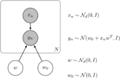
Graphically, a (Bayesian) linear regression can be defined as follows,

Fig. 1: Bayesian Linear Regression The InferPy code for this model is shown below,

@inf.probmodel def linear_reg(d):

w0 = inf.Normal(0, 1, name="w0")

w = inf.Normal(tf.zeros([d,1]), 1, name="w")

x = inf.Normal(tf.ones([d]), 2, name="x") y = inf.Normal(w0 + x @ w, 1.0, name="y")

@inf.probmodel def qmodel(d):

qw0_loc = inf.Parameter(0., name="qw0_loc")

qw0_scale = tf.math.softplus(inf.Parameter(1., name="qw0_scale")) qw0 = inf.Normal(qw0_loc, qw0_scale, name="w0")

qw_loc = inf.Parameter(tf.zeros([d,1]), name="qw_loc")

qw_scale = tf.math.softplus(inf.Parameter(tf.ones([d,1]), name="qw_scale"))

(28)

(continued from previous page) qw = inf.Normal(qw_loc, qw_scale, name="w")

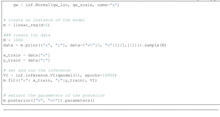
# create an instance of the model m = linear_reg(d=2)

### create toy data N = 1000

data = m.prior(["x", "y"], data={"w0":0, "w":[[2],[1]]}).sample(N)

x_train = data["x"] y_train = data["y"]

# set and run the inference

VI = inf.inference.VI(qmodel(2), epochs=10000) m.fit({"x": x_train, "y":y_train}, VI)

# extract the parameters of the posterior m.posterior(["w", "w0"]).parameters()

7.2 Bayesian Logistic Regression

Graphically, a (Bayesian) logistic regression can be defined as follows,

Fig. 2: Bayesian Linear Regression The InferPy code for this model is shown below,

# required pacakges import inferpy as inf

import numpy as np

@inf.probmodel def log_reg(d):

w0 = inf.Normal(0., 1, name="w0")

w = inf.Normal(0., 1, batch_shape=[d,1], name="w")

x = inf.Normal(0., 2., batch_shape=d, name="x") y = inf.Bernoulli(logits = w0 + x @ w, name="y")

(29)

(continued from previous page)

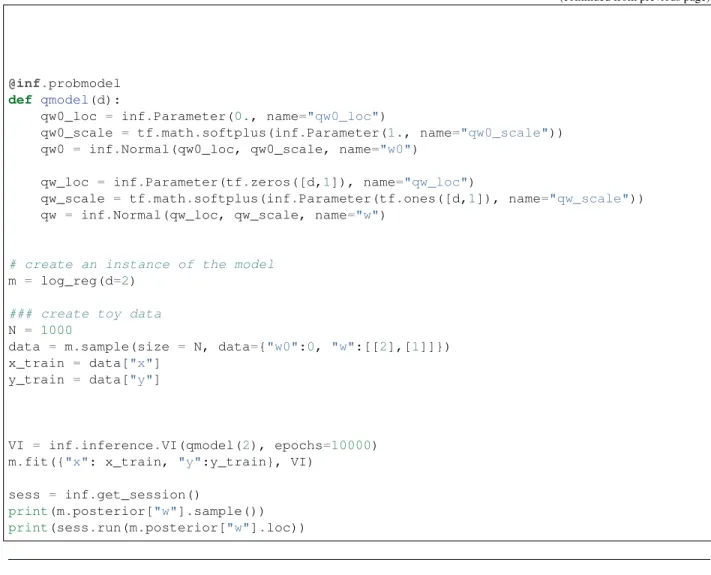
@inf.probmodel def qmodel(d):

qw0_loc = inf.Parameter(0., name="qw0_loc")

qw0_scale = tf.math.softplus(inf.Parameter(1., name="qw0_scale")) qw0 = inf.Normal(qw0_loc, qw0_scale, name="w0")

qw_loc = inf.Parameter(tf.zeros([d,1]), name="qw_loc")

qw_scale = tf.math.softplus(inf.Parameter(tf.ones([d,1]), name="qw_scale")) qw = inf.Normal(qw_loc, qw_scale, name="w")

# create an instance of the model m = log_reg(d=2)

### create toy data N = 1000

data = m.sample(size = N, data={"w0":0, "w":[[2],[1]]}) x_train = data["x"]

y_train = data["y"]

VI = inf.inference.VI(qmodel(2), epochs=10000) m.fit({"x": x_train, "y":y_train}, VI)

sess = inf.get_session()

print(m.posterior["w"].sample())

print(sess.run(m.posterior["w"].loc))

7.3 Linear Factor Model (PCA)

A linear factor model allows to perform principal component analysis (PCA). Graphically, it can be defined as follows,

(30)

The InferPy code for this model is shown below, import inferpy as inf

import numpy as np

# definition of a generic model @inf.probmodel

def pca(k,d):

beta = inf.Normal(loc=tf.zeros([k,d]),

scale=1, name="beta") # shape = [k,d]

z = inf.Normal(tf.ones([k]),1, name="z") # shape = [N,k] x = inf.Normal(z @ beta , 1, name="x") # shape = [N,d]

# create an instance of the model m = pca(k=1,d=2)

@inf.probmodel def qmodel(k,d):

qbeta_loc = inf.Parameter(tf.zeros([k,d]), name="qbeta_loc") qbeta_scale = tf.math.softplus(inf.Parameter(tf.ones([k,d]),

name="qbeta_scale"))

qbeta = inf.Normal(qbeta_loc, qbeta_scale, name="beta")

qz_loc = inf.Parameter(np.ones([k]), name="qz_loc") qz_scale = tf.math.softplus(inf.Parameter(tf.ones([k]),

name="qz_scale"))

VI = inf.inference.VI(qmodel(k=1,d=2), epochs=2000)

# extract the hidden encoding

hidden_encoding = m.posterior("z").parameters()["loc"]

# project x_test into the reduced space (encode) m.posterior("z", data={"x": x_test}).sample(5)

# sample from the posterior predictive (i.e., simulate values for x given the learnt

˓→hidden)

m.posterior_predictive("x").sample(5)

# decode values from the hidden representation

(31)

7.4 Non-linear Factor Model (NLPCA)

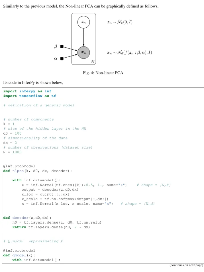
Similarly to the previous model, the Non-linear PCA can be graphically defined as follows,

Fig. 4: Non-linear PCA Its code in InferPy is shown below,

# definition of a generic model

@inf.probmodel

z = inf.Normal(tf.ones([k])*0.5, 1., name="z") # shape = [N,k] output = decoder(z,d0,dx)

h0 = tf.layers.dense(z, d0, tf.nn.relu) return tf.layers.dense(h0, 2 * dx)

@inf.probmodel def qmodel(k):

(32)

(continued from previous page) qz_loc = inf.Parameter(tf.ones([k])_*0.5, name="qz_loc")

# create an instance of the model m = nlpca(k,d0,dx, decoder)

hidden_encoding = m.posterior("z").parameters()["loc"]

# project x_test into the reduced space (encode) m.posterior("z", data={"x": x_test}).sample(5)

# sample from the posterior predictive (i.e., simulate values for x given the learnt

˓→hidden)

m.posterior_predictive("x").sample(5)

# decode values from the hidden representation

m.posterior_predictive("x", data={"z": [2]}).sample(5)

7.5 Variational auto-encoder (VAE)

Similarly to the models PCA and NLPCA, a variational autoencoder allows to perform dimensionality reduction. However a VAE will contain a neural network in the P model (decoder) and another one in the Q (encoder). Its code in InferPy is shown below,

@inf.probmodel

def vae(k, d0, dx, decoder):

(33)

(continued from previous page) z = inf.Normal(tf.ones([k])_*0.5, 1., name="z") # shape = [N,k]

output = decoder(z,d0,dx) x_loc = output[:,:dx]

def decoder(z,d0,dx): _{# k -> d0 -> 2*dx} h0 = tf.layers.dense(z, d0, tf.nn.relu) return tf.layers.dense(h0, 2 _* dx)

def encoder(x, d0, k): _{# dx -> d0 -> 2*k} h0 = tf.layers.dense(x, d0, tf.nn.relu) return tf.layers.dense(h0, 2*k)

@inf.probmodel

def qmodel(k, d0, dx, encoder):

x = inf.Normal(tf.ones([dx]),1,name="x")

output = encoder(x, d0, k) qz_loc = output[:, :k]

qz_scale = tf.nn.softmax(output[:, k:])

# create an instance of the model m = vae(k,d0,dx, decoder)

q = qmodel(k,d0,dx,encoder)

SVI = inf.inference.SVI(q, epochs=5000)

# learn the parameters m.fit({"x": x_train}, SVI)

(34)

(35)

EIGHT

INFERPY PACKAGE

8.1 Subpackages

8.1.1 inferpy.contextmanager package

Submodules inferpy.contextmanager.data_model module

inferpy.contextmanager.data_model.datamodel(size=None)

This context is used to declare a plateau model. Random Variables and Parameters will use a sample_shape defined by the argument size, or by the data_model.fit. If size is not specify, the default size 1, or the size specified byfitwill be used.

inferpy.contextmanager.data_model.fit(size)

inferpy.contextmanager.data_model.get_sample_shape(name)

This function must be used inside a datamodel context (it is not checked here) If var parameters are not expanded, then expand.

name (str) The name of the variable to get its sample shape

returns a the sample_shape (number of samples of the datamodel). It is an integer, or ().

inferpy.contextmanager.data_model.is_active()

inferpy.contextmanager.evidence module

inferpy.contextmanager.evidence.observe(variables,data)

inferpy.contextmanager.randvar_registry module

inferpy.contextmanager.randvar_registry.get_graph()

inferpy.contextmanager.randvar_registry.get_var_parameters() inferpy.contextmanager.randvar_registry.get_variable(name)

inferpy.contextmanager.randvar_registry.get_variable_or_parameter(name) inferpy.contextmanager.randvar_registry.init(graph=None)

inferpy.contextmanager.randvar_registry.is_building_graph() inferpy.contextmanager.randvar_registry.is_default()

(36)

inferpy.contextmanager.randvar_registry.register_parameter(p) inferpy.contextmanager.randvar_registry.register_variable(rv) inferpy.contextmanager.randvar_registry.restart_default()

inferpy.contextmanager.randvar_registry.update_graph(rv_name=None)

Module contents

8.1.2 inferpy.datasets package

Submodules

inferpy.datasets.mnist module MNIST handwritten digits dataset.

inferpy.datasets.mnist.load_data(vectorize=True, num_instances=None, num_instances_test=None, digits=[0, 1, 2, 3, 4, 5, 6, 7, 8, 9])

Loads the MNIST datase Parameters

• vectorize– if true, each 2D image is transformed into a 1D vector • num_instances– total number of images loaded

• digits– list of integers indicating the digits to be considered Returns Tuple of Numpy arrays:‘(x_train, y_train), (x_test, y_test)

inferpy.datasets.mnist.plot_digits(data, grid=[3, 3])

Module contents

8.1.3 inferpy.inference package

Subpackages inferpy.inference.variational package Subpackages inferpy.inference.variational.loss_functions package Submodules inferpy.inference.variational.loss_functions.elbo module

inferpy.inference.variational.loss_functions.elbo.ELBO(pvars, qvars, batch_weight=1,**kwargs)

(37)

expanded p random variables :type pvars: dict<inferpy.RandomVariable>:param qvars: The dict with the ex-panded q random variables :type qvars:dict<inferpy.RandomVariable>:param batch_weight: Weight to assign less importance to the energy, used when processing data in batches :type batch_weight:float

Returns (tf.Tensor): The generated loss tensor

Module contents

inferpy.inference.variational.loss_functions.ELBO(pvars, qvars, batch_weight=1, **kwargs)

Compute the loss tensor from the expanded variables of p and q models. :param pvars: The dict with the expanded p random variables :type pvars: dict<inferpy.RandomVariable>:param qvars: The dict with the ex-panded q random variables :type qvars:dict<inferpy.RandomVariable>:param batch_weight: Weight to assign less importance to the energy, used when processing data in batches :type batch_weight:float

Returns (tf.Tensor): The generated loss tensor

Submodules

inferpy.inference.variational.svi module

class inferpy.inference.variational.svi.SVI(*args,batch_size=100,**kwargs)

Bases:inferpy.inference.variational.vi.VI

compile(pmodel,data_size)

create_input_data_tensor(sample_dict)

update(sample_dict)

inferpy.inference.variational.vi module

class inferpy.inference.variational.vi.VI(qmodel, loss=’ELBO’, opti-mizer=’AdamOptimizer’,epochs=1000)

Bases:inferpy.inference.inference.Inference

log_prob(data)

property losses parameters()

sample(size=1,data={})

Module contents Submodules

inferpy.inference.inference module

class inferpy.inference.inference.Inference

(38)

This class implements the functionality of any Inference class.

log_prob(data)

parameters()

sum_log_prob(data)

Computes the sum of the log probabilities of a (set of) sample(s)

Module contents

Any inference class must implement a run method, which receives a sample_dict object, and returns a dict of posterior objects (random distributions, list of samples, etc.)

class inferpy.inference.SVI(*args,batch_size=100,**kwargs)

Bases:inferpy.inference.variational.vi.VI

create_input_data_tensor(sample_dict)

class inferpy.inference.VI(qmodel,loss=’ELBO’,optimizer=’AdamOptimizer’,epochs=1000)

Bases:inferpy.inference.inference.Inference

log_prob(data)

property losses parameters()

8.1.4 inferpy.models package

Submodules

inferpy.models.parameter module

class inferpy.models.parameter.Parameter(initial_value,name=None)

Bases:object

Random Variable parameter which can be optimized by an inference mechanism.

inferpy.models.prob_model module

class inferpy.models.prob_model.ProbModel(builder)

(39)

Class that implements the probabilistic model functionality. It is composed of a graph, capturing the variable relationships, an OrderedDict containing the Random Variables/Parameters in order of creation, and the function which declare the Random Variables/Parameters.

expand_model(size=1)

Create the expanded model vars using size as plate size and return the OrderedDict

fit(sample_dict,inference_method)

plot_graph()

posterior(target_names=None,data={})

posterior_predictive(target_names=None,data={})

prior(target_names=None,data={})

inferpy.models.prob_model.probmodel(builder)

Decorator to create probabilistic models. The function decorated must be a function which declares the Random Variables in the model. It is not needed that the function returns such variables (we capture them using ed.tape).

inferpy.models.random_variable module

inferpy.models.random_variable.Autoregressive(*args,**kwargs)

Class for random variables. It encapsulates the Random Variable from edward2, and addi-tional properties.

• It creates a variable generator. It must be a function without parameters, that creates a new Random Variable from edward2. It is used to define edward2 models as functions. Also, it is useful to define models using the intercept function.

• The first time the var property is used, it creates a var using the variable generator. Random Variable information:

Create a random variable for Autoregressive. See Autoregressive for more details.

Returns RandomVariable. #### Original Docstring for Distribution Construct anAutoregressivedistribution.

Parameters

• distribution_fn– Pythoncallablewhich constructs a tfd.Distribution-like instance from aTensor(e.g.,sample0). The function must respect the “autoregressive property”, i.e., there exists a permutation of event such that each coordinate is a diffeomorphic function of on preceding coordinates.

• sample0– Initial input todistribution_fn; used to build the distribution in__init__which in turn specifies this distribution’s properties, e.g., event_shape, batch_shape, dtype. If unspecified, thendistribution_fnshould be default constructable.

• num_steps – Number of times distribution_fn is composed from samples, e.g., num_steps=2impliesdistribution_fn(distribution_fn(sample0).sample(n)).sample(). • validate_args– Pythonbool. Whether to validate input with asserts. Ifvalidate_args

(40)

• allow_nan_stats– Pythonbool, defaultTrue. WhenTrue, statistics (e.g., mean, mode, variance) use the value “NaN” to indicate the result is undefined. WhenFalse, an exception is raised if one or more of the statistic’s batch members are undefined.

• name– Pythonstrname prefixed to Ops created by this class. Default value: “Autoregres-sive”.

Raises

• ValueError – if num_steps and num_elements(distribution_fn(sample0).event_shape) are bothNone.

• ValueError– ifnum_steps < 1.

inferpy.models.random_variable.BatchReshape(*args,**kwargs)

Create a random variable for BatchReshape. See BatchReshape for more details.

Returns RandomVariable. #### Original Docstring for Distribution Construct BatchReshape distribution.

Parameters

• distribution– The base distribution instance to reshape. Typically an instance of Distribution.

• batch_shape– Positiveint-like vector-shapedTensorrepresenting the new shape of the batch dimensions. Up to one dimension may contain-1, meaning the remainder of the batch size.

• validate_args– Python bool, defaultFalse. When Truedistribution parameters are checked for validity despite possibly degrading runtime performance. WhenFalseinvalid inputs may silently render incorrect outputs.

• name– The name to give Ops created by the initializer. Default value:“BatchReshape” + distribution.name.

Raises

• ValueError– ifbatch_shapeis not a vector.

• ValueError– ifbatch_shapehas non-positive elements.

• ValueError– ifbatch_shapesize is not the same as adistribution.batch_shapesize.

(41)

Create a random variable for Bernoulli. See Bernoulli for more details.

Returns RandomVariable. #### Original Docstring for Distribution Construct Bernoulli distributions.

Parameters

• logits– An N-DTensorrepresenting the log-odds of a1event. Each entry in the Ten-sorparametrizes an independent Bernoulli distribution where the probability of an event is sigmoid(logits). Only one oflogitsorprobsshould be passed in.

• probs– An N-DTensorrepresenting the probability of a1event. Each entry in theTensor parameterizes an independent Bernoulli distribution. Only one oflogitsorprobsshould be passed in.

• dtype– The type of the event samples. Default:int32.

• name– Pythonstrname prefixed to Ops created by this class. Raises ValueError– If p and logits are passed, or if neither are passed.

inferpy.models.random_variable.Beta(*args,**kwargs)

Create a random variable for Beta. See Beta for more details.

Returns RandomVariable. #### Original Docstring for Distribution Initialize a batch of Beta distributions.

(42)

Parameters

• concentration1– Positive floating-pointTensorindicating mean number of successes; aka “alpha”. Impliesself.dtypeandself.batch_shape, i.e.,concentration1.shape = [N1, N2, . . . , Nm] = self.batch_shape.

• concentration0– Positive floating-pointTensorindicating mean number of failures; aka “beta”. Otherwise has same semantics asconcentration1.

• name– Pythonstrname prefixed to Ops created by this class.

inferpy.models.random_variable.Binomial(*args,**kwargs)

Create a random variable for Binomial. See Binomial for more details.

Returns RandomVariable. #### Original Docstring for Distribution Initialize a batch of Binomial distributions.

Parameters

• total_count– Non-negative floating point tensor with shape broadcastable to[N1,. . . , Nm]withm >= 0and the same dtype asprobsorlogits. Defines this as a batch ofN1 x . . . x Nmdifferent Binomial distributions. Its components should be equal to integer values. • logits– Floating point tensor representing the log-odds of a positive event with shape

broadcastable to [N1,. . . , Nm] m >= 0, and the same dtype astotal_count. Each entry represents logits for the probability of success for independent Binomial distributions. Only one oflogitsorprobsshould be passed in.

• probs– Positive floating point tensor with shape broadcastable to[N1,. . . , Nm] m >= 0, probs in [0, 1]. Each entry represents the probability of success for independent Binomial distributions. Only one oflogitsorprobsshould be passed in.

(43)

inferpy.models.random_variable.Blockwise(*args,**kwargs)

Create a random variable for Blockwise. See Blockwise for more details.

Returns RandomVariable. #### Original Docstring for Distribution Construct theBlockwisedistribution.

Parameters

• distributions– Python list of tfp.distributions.Distribution instances. All distribu-tion instances must have the samebatch_shapeand all must haveevent_ndims==1, i.e., be vector-variate distributions.

• dtype_override– samples ofdistributionswill be cast to thisdtype. If unspecified, all distributionsmust have the samedtype. Default value:None(i.e., do not cast).

inferpy.models.random_variable.Categorical(*args,**kwargs)

Create a random variable for Categorical. See Categorical for more details.

Returns RandomVariable. #### Original Docstring for Distribution

(44)

Parameters

• logits– An N-DTensor,N >= 1, representing the log probabilities of a set of Categorical distributions. The firstN - 1dimensions index into a batch of independent distributions and the last dimension represents a vector of logits for each class. Only one oflogitsorprobs should be passed in.

• probs– An N-DTensor,N >= 1, representing the probabilities of a set of Categorical distributions. The firstN - 1dimensions index into a batch of independent distributions and the last dimension represents a vector of probabilities for each class. Only one oflogitsor probsshould be passed in.

• dtype– The type of the event samples (default: int32).

inferpy.models.random_variable.Cauchy(*args,**kwargs)

Create a random variable for Cauchy. See Cauchy for more details.

Returns RandomVariable. #### Original Docstring for Distribution Construct Cauchy distributions.

The parameters locandscalemust be shaped in a way that supports broadcasting (e.g. loc + scale is a valid operation).

Parameters

• loc– Floating point tensor; the modes of the distribution(s).

• scale– Floating point tensor; the locations of the distribution(s). Must contain only posi-tive values.

(45)

• name– Pythonstrname prefixed to Ops created by this class. Raises TypeError– iflocandscalehave differentdtype.

inferpy.models.random_variable.Chi(*args,**kwargs)

Create a random variable for Chi. See Chi for more details.

Returns RandomVariable. #### Original Docstring for Distribution Construct Chi distributions with parameterdf.

Parameters

• df– Floating point tensor, the degrees of freedom of the distribution(s). df must contain only positive values.

• allow_nan_stats– Pythonbool, defaultTrue. WhenTrue, statistics (e.g., mean, mode, variance) use the valueNaNto indicate the result is undefined. WhenFalse, an exception is raised if one or more of the statistic’s batch members are undefined.

• name– Pythonstrname prefixed to Ops created by this class. Default value:‘Chi’.

inferpy.models.random_variable.Chi2(*args,**kwargs)

Create a random variable for Chi2. See Chi2 for more details.

Returns RandomVariable. #### Original Docstring for Distribution Construct Chi2 distributions with parameterdf.

(46)

• df– Floating point tensor, the degrees of freedom of the distribution(s). df must contain only positive values.

inferpy.models.random_variable.Chi2WithAbsDf(*args,**kwargs)

Create a random variable for Chi2WithAbsDf. See Chi2WithAbsDf for more details.

Returns RandomVariable. #### Original Docstring for Distribution DEPRECATED FUNCTION

Warning: THIS FUNCTION IS DEPRECATED. It will be removed after 2019-06-05. Instructions for updating: Chi2WithAbsDf is deprecated, use Chi2(df=tf.floor(tf.abs(df))) instead.

inferpy.models.random_variable.ConditionalDistribution(*args,**kwargs)

Create a random variable for ConditionalDistribution. See ConditionalDistribution for more details.

Returns RandomVariable. #### Original Docstring for Distribution Constructs theDistribution.

This is a private method for subclass use. Parameters

(47)

• reparameterization_type – Instance of ReparameterizationType. If tfd.FULLY_REPARAMETERIZED, this Distribution can be reparameterized in terms of some standard distribution with a function whose Jacobian is constant for the support of the standard distribution. Iftfd.NOT_REPARAMETERIZED, then no such reparameteriza-tion is available.

• parameters– Pythondictof parameters used to instantiate thisDistribution. • graph_parents– Pythonlistof graph prerequisites of thisDistribution.

• name– Pythonstrname prefixed to Ops created by this class. Default: subclass name. Raises ValueError– if any member of graph_parents isNoneor not aTensor.

inferpy.models.random_variable.ConditionalTransformedDistribution(*args, **kwargs)

Create a random variable for ConditionalTransformedDistribution. See ConditionalTransformedDistribution for more details.

Returns RandomVariable. #### Original Docstring for Distribution Construct a Transformed Distribution.

Parameters

• distribution– The base distribution instance to transform. Typically an instance of Distribution.

• bijector– The object responsible for calculating the transformation. Typically an in-stance ofBijector.

• batch_shape– integervectorTensor which overrides distribution batch_shape; valid only ifdistribution.is_scalar_batch().

• event_shape– integervector Tensor which overrides distribution event_shape; valid only ifdistribution.is_scalar_event().

• kwargs_split_fn– Pythoncallablewhich takes a kwargsdictand returns a tuple of kwargsdict‘s for each of the ‘distribution andbijector parameters respectively. Default value:_default_kwargs_split_fn(i.e.,

‘lambda kwargs: (kwargs.get(‘distribution_kwargs’, {}), kwargs.get(‘bijector_kwargs’, {}))‘)

(48)

• parameters– Locals dict captured by subclass constructor, to be used for copy/slice re-instantiation operations.

• name– Pythonstrname prefixed to Ops created by this class. Default: bijector.name + distribution.name.

inferpy.models.random_variable.Deterministic(*args,**kwargs)

Create a random variable for Deterministic. See Deterministic for more details.

Returns RandomVariable. #### Original Docstring for Distribution Initialize a scalarDeterministicdistribution.

Theatolandrtolparameters allow for some slack inpmf,cdf computations, e.g. due to floating-point error.

‘‘‘ pmf(x; loc)

= 1, if Abs(x - loc) <= atol + rtol * Abs(loc), = 0, otherwise.

‘‘‘

Parameters

• loc– NumericTensorof shape[B1, . . . , Bb], withb >= 0. The point (or batch of points) on which this distribution is supported.

• atol– Non-negativeTensorof samedtypeaslocand broadcastable shape. The absolute tolerance for comparing closeness toloc. Default is0.

• rtol– Non-negativeTensorof samedtypeas locand broadcastable shape. The relative tolerance for comparing closeness toloc. Default is0.

inferpy.models.random_variable.Dirichlet(*args,**kwargs)

(49)

Create a random variable for Dirichlet. See Dirichlet for more details.

Returns RandomVariable. #### Original Docstring for Distribution Initialize a batch of Dirichlet distributions.

Parameters

• concentration– Positive floating-pointTensor indicating mean number of class oc-currences; aka “alpha”. Impliesself.dtype, andself.batch_shape, self.event_shape, i.e., if concentration.shape = [N1, N2, . . . , Nm, k]thenbatch_shape = [N1, N2, . . . , Nm] and event_shape = [k].

inferpy.models.random_variable.DirichletMultinomial(*args,**kwargs)

Create a random variable for DirichletMultinomial. See DirichletMultinomial for more details.

Returns RandomVariable. #### Original Docstring for Distribution

Initialize a batch of DirichletMultinomial distributions. Parameters

• total_count– Non-negative floating point tensor, whose dtype is the same as concen-tration. The shape is broadcastable to[N1,. . . , Nm]withm >= 0. Defines this as a batch of N1 x . . . x Nmdifferent Dirichlet multinomial distributions. Its components should be equal to integer values.