A New Approach to
Dynamic All Pairs Shortest Paths
∗
Camil Demetrescu
†Giuseppe F. Italiano
‡Abstract
We study novel combinatorial properties of graphs that allow us to devise a com-pletely new approach to dynamic all pairs shortest paths problems. Our approach yields a fully dynamic algorithm for general directed graphs with non-negative real-valued edge weights that supports any sequence of operations inO(n2log3n) amortized time per update and unit worst-case time per distance query, wherenis the number of vertices. We can also report shortest paths in optimal worst-case time. These bounds improve substantially over previous results and solve a long-standing open problem. Our algorithm is deterministic, uses simple data structures, and appears to be very fast in practice.
1
Introduction
In this paper we present fully dynamic algorithms for maintaining all pairs shortest paths (APSP) in directed graphs withreal-valuededge weights. A dynamic graph algorithm main-tains a given property P on a weighted graph subject to dynamic changes, such as edge insertions, edge deletions and edge weight updates. Note that edge deletions and edge inser-tions can be easily formulated as edge weight updates, by setting to +∞the weight of edges not in the graph. A dynamic graph algorithm should process queries on property P quickly, and must perform update operations faster than recomputing the solution from scratch, as
∗This work has been partially supported by the Sixth Framework Programme of the EU under contract
number 507613 (Network of Excellence “EuroNGI: Designing and Engineering of the Next Generation In-ternet”), by the IST Programme of the EU under contract n. IST-1999-14186 (ALCOM-FT), by the HPRN Programme of the EU under contract n. HPRN-CT-1999-00104 (AMORE), and by the Italian Ministry of University and Research (Project “ALINWEB: Algorithmics for Internet and the Web”). A preliminary ver-sion of this paper was presented at the35th Annual ACM Symposium on Theory of Computing (STOC’03)[6]. The final remarks of the conference version claimed that anO(n2log2n) update bound could be achieved
for fully dynamic all pairs shortest paths; however, this claim was supported with inaccurate arguments.
†Dipartimento di Informatica e Sistemistica, Universit`a di Roma “La Sapienza”, Roma, Italy. Email:
demetres@dis.uniroma1.it. URL: http://www.dis.uniroma1.it/~demetres.
‡Dipartimento di Informatica, Sistemi e Produzione, Universit`a di Roma “Tor Vergata”, Roma,
Italy and Centro “Vito Volterra”, Universit`a di Roma “Tor Vergata”, Roma, Italy. Email:
carried out by the fastest static algorithm. We say that an algorithm is fully dynamic if it can handle both edge weight increases and edge weight decreases. A partially dynamic algorithm can handle either edge weight increases or decreases, but not both.
The Problem. In the fully dynamic APSP problem that we consider we wish to maintain a directed graph with real-valued edge weights under an intermixed sequence of the following operations:
update(v, w0): update the weights of all edges incident to vertex v according to
weight function w0.
distance(x, y): return the distance from vertex x to vertex y.
path(x, y): report a shortest path from vertex x to vertex y, if any.
Notice that in this paper we consider a generalized version of the dynamic all pairs shortest path problem where the weights of all edges incident to a given vertex can be changed with just one update operation. In the following we will call such operation vertex update. We recall that in this setting, edge deletions can be modeled by raising edge weights to +∞, while edge insertions can be realized by decreasing edge weights from +∞ to a finite value. Throughout the paper, we denote by n the number of vertices in the graph and by m the number of edges with weights <+∞in the graph.
Previous Work. The dynamic maintenance of shortest paths has a remarkably long his-tory, as the first papers date back to over 35 years ago [13, 14, 17]. After that, many dynamic shortest paths algorithms have been proposed (see e.g., [7, 9, 10, 15, 16, 18]), but their running times in the worst case were comparable to recomputing APSP from scratch. The first dynamic shortest path algorithms which are provably faster than recomputing APSP from scratch only worked on graphs with small integer weights. In particular, Ausiello et al.[1] proposed a decrease-only shortest path algorithm for directed graphs having positive integer weights less than C: the amortized running time of their algorithm is O(Cnlogn) per edge insertion. Henzinger et al. [11] designed a fully dynamic algorithm for APSP on planar graphs with integer weights, with a running time of O(n4/3log(nC)) per operation. Recently, Fakcharoemphol and Rao in [8] designed a fully dynamic algorithm for maintaining single-source shortest paths in planar directed graphs that supports both queries and edge weight updates in O(n4/5log13/5n) amortized time per edge operation.
The first big step on general graphs and integer weights was made by King [12], who presented a fully dynamic algorithm for maintaining all pairs shortest paths in directed graphs with positive integer weights less than C: the running time of her algorithm is O(n2.5√Clogn) per update. In previous work [4, 5], we have solved fully dynamic APSP on general directed graphs with real weights. In particular, given a directed graphG, subject to dynamic operations, and such that each edge weight can take at most S different real values, we proposed a deterministic algorithm that supports each update inO(n2.5qSlog3
amortized time and each query inO(1) worst-case time. Other deletions-only algorithms for APSP, in the simpler case of unweighted graphs, are presented in [2].
Our Results. We study novel combinatorial properties of graphs that allow us to devise a completely new approach to dynamic all pairs shortest paths. This approach yields a fully dynamic algorithm for APSP on general directed graphs with non-negative real-valued edge weights that achieves the following time bounds: it supports any sequence of operations in O(n2log3
n) amortized time per update and one look-up in the worst case per distance query; it can also report shortest paths in optimal worst-case time. We remark that our algorithm improves substantially over previous bounds [4, 5, 12]. Furthermore, and unlike all the previous approaches, it solves fully dynamic APSP in its generality. Indeed, it runs on (non-negative) real weights, and each weight has no limit on the number of different values it can take. Finally, we note that when the distance matrix has to be maintained explicitly, i.e., distance queries have to be answered with exactly one look-up, as many as Ω(n2) entries of the distance matrix can change during each update. Thus, in this model our algorithm is only a polylogarithmic factor away from the best possible bound. In the special case of increase-only update sequences, our techniques yield a faster update algorithm that runs in O(n2logn) amortized time per operation. Similarly to the fully dynamic case, no previous general solution was known for this problem.
Another interesting feature of our techniques is that both weight increases and weight decreases can be supported with exactly the same code. Surprisingly, our algorithms are rather simple and thus amenable to efficient implementations: indeed, according to a recent experimental study [3], the techniques described in this paper are not only asymptotically efficient, but can yield very fast implementations in many practical scenarios.
Notation. Let G = (V, E) be a directed graph with real edge weights and no negative-length cycles. A path πxy =hx0, x1, . . . , xki from vertex x to vertex y in G is a sequence of vertices such that x0 =x, xk =y, and (xi, xi+1)∈E, for each i, 0≤i < k. Let (u, v) be an edge in E: we denote by wuv the weight of edge (u, v). Let πxy =hx0, x1, . . . , xki be a path in G: we denote by
w(πxy) = kX−1 i=0
wxixi+1
the weight of πxy. We assume that as a special case, πxx =hxi is a path of weight zero. Given πxv = hx, . . . , x0, vi and πvy = hv, y0, . . . , yi, we denote by πxv · πvy the path
hx, . . . , x0, v, y0, . . . , yi obtained by concatenating π
xv and πvy at v. Moreover, we denote by `(πxy) the path πxb such that πxy = πxb· hb, yi. Similarly, we denote by r(πxy) the path πay such that πxy =hx, ai ·πay.
Let the graph G be subject to a sequence of (vertex) updates Σ = hσ1, σ2, . . . , σki. We denote bytσi the time immediately after updateσi, withtσi =ifor anyi, 1≤i≤k. We also
denote by vσ the vertex affected by the update σ: i.e., if σ = update(x, w0), then vσ = x. The notation used in this paper is summarized in Table 1.
G= (V, E) weighted directed graph with vertex set V and edge set E wuv weight of edge (u, v)
πxy =hx, . . . , yi path from vertex x to vertexy
w(πxy) weight of path πxy (sum of the weights of the edges in πxy) `(πxy) subpath πxb of πxy such that πxy =πxb· hb, yi
r(πxy) subpath πay of πxy such that πxy =hx, ai ·πay Σ =hσ1, σ2, . . . , σki sequence of update operations
tσ time at which update σ occurs vσ vertex affected by update σ
Table 1: Notation used in the paper.
Throughout the paper we assume that there is only one shortest path between each pair of vertices in G. This is without loss of generality, since ties can be broken consistently as we will discuss in Section 3.4.
Organization of the Paper. The remainder of this paper is organized as follows. Sec-tion 2 studies some properties of special classes of paths in a graph, while SecSec-tion 3 shows how to exploit them to devise the first general increase-only update algorithm for all pairs shortest paths. To deal with fully dynamic sequences, Section 4 addresses more path proper-ties, which are next used in Section 5 to devise the first general algorithm for fully dynamic all pairs shortest paths. We remark that, while Section 2 and Section 4 contain combinatorial results on graphs, algorithmic aspects are treated in Section 3 and Section 5. We conclude the paper in Section 6 with some remarks and directions for further research.
2
Locally Shortest Paths
In this section we study the properties of a class of paths in a graph that we call locally shortest paths. Using this notion, in Section 3 we will show how to maintain efficiently all pairs shortest paths in a graph subject to partially dynamic edge weight updates. Locally shortest paths are defined as follows.
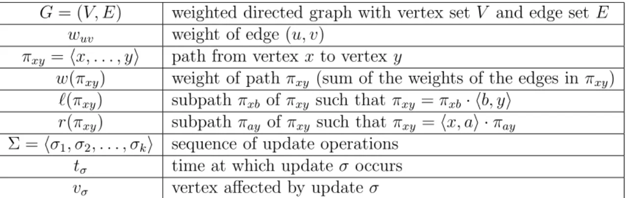
Definition 1 A path πxy is Locally Shortest1 in G if either: (i) πxy consists of a single vertex, or
(ii) every proper subpath of πxy is a shortest path in G.
This definition is inspired by the optimal-substructure property of shortest paths: all sub-paths of a shortest path are shortest sub-paths. Here, we relax this property by considering only 1Since every internal vertex of a locally shortest path has the same sum of distances to the endpoints, in
proper subpaths. Indeed, in a locally shortest path, all proper subpaths are shortest paths: however, the path itself may not necessarily be shortest. We assume that every trivial path formed by a single vertex or a single edge is locally shortest. Notice that, by the optimal substructure of shortest paths, it is possible to check whether a non-trivial pathπxy is locally shortest by just verifying that `(πxy) and r(πxy) are shortest paths in G. In the remainder of this section we discuss some properties of locally shortest paths.
Lemma 1 If we denote by SP and LSP respectively the sets of shortest paths and locally shortest paths in G, then SP ⊆LSP.
Proof. Every subpath of a shortest path is a shortest path itself. Thus every shortest path
is trivially a locally shortest path. 2
Lemma 2 If shortest paths are unique in G, then for each pair of vertices x and y, the locally shortest paths connecting x and y in G are internally vertex-disjoint, i.e., except for the endpoints, they use different vertices.
Proof. Suppose by contradiction that there exist two distinct locally shortest pathsπxy1 and π2
xy that are not internally vertex-disjoint. This means that there is some vertex v, with v 6= x and v 6= y, that belongs to both π1
xy and πxy2 . Since shortest paths are unique, then there is only one shortest path πxv from x to v, and only one shortest path πvy from v to y. Since every proper subpath of π1
xy and πxy2 is shortest, then πxv and πvy are necessarily subpaths of both π1
xy and πxy2 . Thus, π1xy =πxy2 , which contradicts our initial assumption. 2
Lemma 3 If shortest paths are unique in G, then there can be at most mn locally shortest paths in G.
Proof. Fix an edge (x, v) and a vertex y inG. We first note that there can be at most one locally shortest pathπxy =hx, v, . . . , yistarting from edge (x, v). This derives from the fact that every proper subpath of πxy must be shortest (Definition 1), and from the uniqueness of shortest paths. Since the first edge (x, v) can be chosen in m different ways and the destination vertex y can be chosen among n different vertices, at any time there can be at
most mn locally shortest paths inG. 2
We now study how the set of locally shortest paths changes in a graph subject to partially dynamic updates such as vertex increases, i.e., operations that increase the weights of all edges incident to it, or vertex decreases, i.e., operations that decrease the weights of all edges incident to it.
Lemma 4 Let G be a graph subject to a sequence Σ of vertex updates. If shortest paths are unique in G, then in the worst case at most O(n2) paths can stop being locally shortest due to a vertex increase.
Proof. We observe that a path can stop being locally shortest only if any of its proper subpaths stops being shortest. In case of increases, this can happen only if that subpath contains the updated vertex, say vertexv. By Lemma 2, there can be at most O(n2) locally shortest paths that containv as an internal vertex. Furthermore, there can be at mostO(n2) locally shortest paths starting or ending in v. This yields a total of at most O(n2) paths that can stop being locally shortest because of a weight increase in v. 2 Theorem 1 Let G be a graph subject to a sequence Σ of increase-only vertex update oper-ations and let m be the maximum number of edges in G throughout sequence Σ. If shortest paths are unique in G, then the number of paths that start being locally shortest after each update is:
(1) O(mn) in the worst case.
(2) O(n2) amortized over Ω(m/n) update operations.
Proof. Claim (1) follows immediately from Lemma 3. To prove Claim (2), we assign a debit to each locally shortest path in the graph. The debit is paid for by the operation that makes it stop being locally shortest. By Lemma 4, at most O(n2) paths can stop being locally shortest at each update. Moreover, by Lemma 3 there can be at most mn locally shortest paths in a graph at any time, so the total unpaid debit at the end of the sequence never exceeds mn. Thus, the amortized number of paths that start being locally shortest after each update in any sequence of Ω(m/n) operations can be at most O(n2).
2 Notice that both the statements and the proofs of Lemma 4 and Theorem 1 hold sym-metrically if we replace “increase” by “decrease” and swap “start” with “stop”. This can be intuitively explained by observing that, if we replay a decrease-only sequence backwards starting from the final graph, each vertex decrease in the forward sequence corresponds to a symmetric vertex increase in the backward sequence that undoes edge weights back to their previous values. In this scenario, a path starts being locally shortest during a decrease in the forward sequence if and only if it stops being locally shortest during the corresponding increase in the backward sequence, and thus the counting argument holds in both directions.
3
Partially Dynamic Shortest Paths
We now show how to exploit the properties of locally shortest paths discussed in Section 2 to devise an increase-only update algorithm for all pairs shortest paths that runs inO(n2logn) amortized time per operation. To the best of our knowledge, this is the first general result for increase-only all pairs shortest paths that is faster than recomputing the solution from scratch after each update. This is rather surprising compared to the decrease-only case, where an O(n2) bound can be immediately obtained by just running a single-source computation from the updated vertexv to every other vertex, and a single-sink computation from every vertex tov; by doing so, for each pair of vertices x and y, we find a shortest path π∗
and a shortest path π∗
vy from v to y: if π0xy =πxv∗ ·π∗vy is shorter than the previous shortest path πxy from x toy, we simply replace πxy with πxy0 .
Although the update algorithm that we describe below works also for decreases, for the sake of simplicity in this section we analyze the algorithm in the case of increases only. The approach is very simple: we maintain all the locally shortest paths of the underlying graph. By Theorem 1, changes in the data structure will be O(n2) per update in an increase-only sequence of Ω(m/n) operations. We will maintain locally shortest paths in priority queues, and thus we will pay O(logn) for each path that starts/stops being locally shortest. This will yield an O(n2logn) amortized time per update. Even though the combinatorial results discussed in Section 2 impose no restrictions on the edge weights (provided that shortest paths are unique) our algorithm requires that all the edge weights in the graph are non-negative.
3.1
Data Structure
For each pair of vertices xandy inGwe maintain the weight wxy ≥0 of edge (x, y) (or +∞ if no such edge exists) and the following two data structures:
Pxy ={ πxy : πxy is a locally shortest path in G} P∗
xy ={ πxy : πxy is a shortest path in G }
We maintain eachPxy as a priority queue where itemπxy ∈Pxy has priorityw(πxy). We note that, if shortest paths are unique, |P∗
xy| ≤ 1. Furthermore, since by Lemma 1 any shortest path is locally shortest, then for each pair of vertices x and y, P∗
xy ⊆ Pxy. Therefore, a minimum weight path in Pxy is a shortest path. We also observe that each path πxy in Pxy andP∗
xy can be represented implicitly with constant space by just storing two pointers to the subpaths `(πxy) and r(πxy). This is correct by the optimal-substructure property of locally shortest paths and by the assumption of uniqueness of shortest paths. Finally, for each path πxy stored in Pxy we maintain w(πxy) and the following four lists:
L(πxy) = { πx0y =hx0, xi ·πxy : (x0, x)∈E and πx0y is a locally shortest path inG } L∗(πxy) = { πx0y =hx0, xi ·πxy : (x0, x)∈E and πx0y is a shortest path in G}
R(πxy) = { πxy0 =πxy· hy, y0i : (y, y0)∈E and πxy0 is a locally shortest path inG} R∗(πxy) = { πxy0 =πxy· hy, y0i : (y, y0)∈E and πxy0 is a shortest path inG}
In other words,L(πxy) andL∗(πxy) represent pre-extensions ofπxy, whileR(πxy) andR∗(πxy) represent post-extensions of πxy. Once again, by Lemma 1 any shortest path is locally shortest, and thus for each path πxy stored in Pxy,L∗(πxy)⊆L(πxy) and R∗(πxy)⊆R(πxy). For the sake of simplicity, in the following we will sometimes writeP orP∗ instead ofP
xy or P∗
xy whenever the meaning is clear from the context. The notation introduced in this section is summarized in Table 2.
3.2
Implementation of Operations
The distance(x, y) andpath(x, y) operations can be implemented as shown in Figure 1, by simply accessing the minimum weight path in Pxy. Since each Pxy is a subset of the paths in G, the correctness of query operations follows directly from Lemma 1.
distance(x, y):
1. if Pxy =∅ then return+∞
2. else returnthe weight of a minimum weight path in Pxy
path(x, y):
1. if Pxy =∅ then return∅
2. else returna minimum weight path in Pxy
Figure 1: Implementation ofdistance and path operations.
The implementation of the update(v, w0) operation is shown in Figure 2. The update
works in two steps: cleanup and fixup. To simplify the description, we say that a path that is shortest (resp., locally shortest) after the update is new either if it was not shortest (resp., locally shortest) before the update, or if it contains the updated vertex v. We now describe procedures cleanup and fixup in more detail; pseudo-code is given in Figure 2. cleanup(v)
The procedure removes every pathπxy containing vertexvfromPxy,Pxy∗ ,L(r(πxy)),L∗(r(πxy)), R(`(πxy)), and R∗(`(πxy)). Namely, we remove from the data structure all the paths that would stop being locally shortest if we deleted v from the graph. This task can be accom-plished iteratively by first removing paths of the formhu, viandhv, ui, and then by removing all paths listed in L(πxy) and R(πxy) for each path πxy removed in the previous iterations.
fixup(v, w0)
The procedure adds to the data structure all the new shortest and locally shortest paths. It works in three phases, as follows.
Pxy set of locally shortest paths from x toy in G P∗
xy set of shortest paths fromx to y inG
L(πxy) set of pre-extensions hx0, xi ·πxy of πxy that are locally shortest paths in G L∗(π
xy) set of pre-extensions hx0, xi ·πxy of πxy that are shortest paths in G
R(πxy) set of post-extensions πxy· hy, y0iof πxy that are locally shortest paths in G R∗(π
xy) set of post-extensions πxy· hy, y0iof πxy that are shortest paths in G Table 2: Notation introduced in Section 3.1.
update(v, w0): 1. cleanup(v) 2. fixup(v, w0) cleanup(v): 1. Q← {hvi} 2. while Q6=∅ do
3. extract any π from Q
4. for each πxy ∈L(π)∪R(π) do
5. addπxy to Q
6. remove πxy from Pxy,L(r(πxy)), and R(`(πxy))
7. ifπxy ∈Pxy∗ thenremove πxy from Pxy∗ ,L∗(r(πxy)), andR∗(`(πxy))
fixup(v, w0):
1. for each u6=v do {Phase 1}
2. wuv←wuv0 ; wvu ←wvu0 3. ifwuv<+∞ then 4. w(hu, vi)←wuv; `(hu, vi)← hui; r(hu, vi) ← hvi 5. add hu, vi to Puv,L(hvi), and R(hui) 6. ifwvu<+∞ then 7. w(hv, ui)←wvu; `(hv, ui)← hvi; r(hv, ui)← hui 8. add hv, ui to Pvu,L(hui), and R(hvi) 9. H ← ∅ {Phase 2} 10. for each (x, y) do
11. add πxy ∈Pxy with minimum w(πxy) to H
12. while H6=∅ do {Phase 3}
13. extract πxy from H with minimum w(πxy)
14. ifπxy is the first extracted path for pair (x, y) then
15. ifπxy 6∈P∗ xy then 16. add πxy to Pxy∗ ,L∗(r(πxy)), and R∗(`(πxy)) 17. for each πx0b∈L∗(`(πxy)) do 18. πx0y ← hx0, xi ·πxy 19. w(πx0y)←wx0x+w(πxy); `(πx0y)←πx0b; r(πx0y)←πxy 20. add πx0y to Px0y, L(πxy),R(πx0b), andH 21. for each πay0 ∈R∗(r(πxy))do 22. πxy0 ←πxy· hy, y0i 23. w(πxy0)←w(πxy) +wyy0; `(πxy0)←πxy; r(πxy0)←πay0 24. add πxy0 to Pxy0, L(πay0),R(πxy), andH
Phase 1: Sets the weight of every edge (u, v) entering v to the new value w0
uv (line 2). If w0
uv < +∞, then the trivial path πuv = hu, vi is added to Puv, L(r(πuv)), and R(`(πuv)) (lines 3–5). Similar steps are performed for every edge of the form (v, u) (line 2 and lines 6– 8). Thus, all the new locally shortest paths formed by one edge are added to the data structure. Longer new paths will be added in Phase 3.
Phase 2: Initializes a priority queue H with the minimum weight path πxy ∈ Pxy for each pair of vertices (x, y) (lines 9–11);
Phase 3: Repeatedly extracts paths πxy from H in increasing weight order (line 13). The first extracted path for each pair (x, y) is a shortest path between x and y (see Invariant 1 below), while paths extracted later on for the same pair are ignored (line 14). Whenever a shortest path πxy is extracted, we check whether πxy is already in Pxy∗ (line 15). If not, we add πxy to Pxy∗ , L∗(r(πxy)), and R∗(`(πxy)) (line 16), and we combine it with existing shortest paths to form new locally shortest paths (lines 17–24). This is done by scanning all paths πx0b listed in L∗(`(πxy)) (line 17) and all paths πay0 listed in R∗(r(πxy)) (line 21), forming the new locally shortest pathsπx0y =hx0, xi ·πxy (lines 18–19) andπxy0 =πxy· hy, y0i (lines 22–23). Each new locally shortest path πij is added to Pij, L(r(πij)), R(`(πij)), and H as soon as it is discovered (line 20 and line 24).
3.3
Analysis
To prove the correctness ofupdate, we assume thatP andP∗are correct before the operation,
and we show that they are also correct afterwards. Operations on the other data structures are simple bookkeeping operations and their correctness can be easily checked. We first discuss an invariant maintained by procedure fixup.
Invariant 1 If shortest paths are unique and edge weights are non-negative, then for each pair of vertices x and y in G, the first path connecting x and y extracted fromH in Phase 3 of fixup is a shortest path.
Proof. Suppose by contradiction that at some extraction the invariant is violated, and the first path πbxy extracted for some pair (x, y) is not a shortest path. Consider the earliest of these events, and letπxy be the unique shortest path betweenxandy, withw(πxy)< w(πbxy). Clearly, πxy 6∈ H, otherwise it would have been extracted in place of πbxy. Moreover, πxy 6∈ Pxy, otherwise it would have been inserted inHinPhase2, being a shortest path. Therefore, πxy has to be necessarily a new locally shortest path, but since in Phase 1 we add to P all the edges incident to v, it cannot be one of them. This implies that πxy contains at least two edges and either one of `(πxy) orr(πxy) is a new shortest path and was not inP∗ at the beginning of fixup. As edge weights are non-negative, then w(`(πxy)) ≤ w(πxy) < w(πbxy) and w(r(πxy)) ≤ w(πxy) < w(πbxy). Since paths are extracted from H in increasing weight order, shortest paths are unique, and all the extractions before the wrong extraction are correct, then either `(πxy) or r(πxy) should have been extracted from H and added to P∗ before the wrong extraction. This implies that πxy should have been formed and inserted in
H at the extraction time of either one of`(πxy) orr(πxy). Soπxy should have been extracted before πbxy, contradicting the assumption that the invariant is violated. 2
Theorem 2 If the operation is an increase, shortest paths are unique, and edge weights are non-negative, then algorithm update correctly updates Pxy and Pxy∗ for each pair of vertices x and y.
Proof. We first observe that cleanup(v) removes from the data structures every locally shortest path that contains the updated vertex v. Thus, since only paths containing v can stop being shortest after an increase, then every path πxy that is no longer locally shortest after the update is removed from Pxy, and possibly from Pxy∗ .
We now show that every new locally shortest path πxy is added to Pxy by fixup(v, w0). Pathsπuv andπvumade of one edge are correctly added toPuvandPvu inPhase 1: therefore, we only focus on paths πxy with at least two edges. We recall that each such path πxy has to be added toPxy if both`(πxy) andr(πxy) are shortest paths after the update, but at least one of them (say`(πxy)) was not inP∗ beforefixup. By Invariant 1, the first extracted path for each pair is shortest, and then `(πxy) is certainly extracted and added to P∗ at some iteration in Phase 3. A that time, `(πxy) is correctly combined with r(πxy) ∈R∗(r(`(πxy))) to form πxy, which is added to Pxy.
To conclude the proof, we observe that by Invariant 1 all shortest paths are extracted at some iteration and are added to P∗, if they are not already there. 2
To conclude the analysis, we address the running time and the space usage of our imple-mentation.
Theorem 3 In an increase-only sequence ofΩ(m/n)operations, if shortest paths are unique and edge weights are non-negative, our data structure supports each update operation in O(n2logn) amortized time, and each distance and path query in optimal time. The space used is O(mn).
Proof. The bounds for queries are immediate, since the minimum weight path in the priority queue Pxy can be retrieved in optimal time.
Since each iteration of cleanup removes a path πxy from a constant number of lists and priority queues, it requires O(logn) time in the worst case. By Lemma 2, at most O(n2) locally shortest paths can go through the updated vertex in the worst case, and thuscleanup will perform at most O(n2) iterations, thus spending at most O(n2logn) time.
Next, it is easy to see that Phase 1 of fixup requires O(nlogn) time in the worst case. To bound the time required by Phase 2 of fixup, we consider that finding the minimum in Pxy takes constant time and each insertion in H takes O(logn) time. This gives a total bound ofO(n2logn) for this phase. Finally, we note that a pathπ
xy is a new locally shortest path if and only if both `(πxy) = hx, . . . , bi ∈ Pxb∗ and r(πxy) = ha, . . . , yi ∈ Pay∗ after the update, and either `(πxy) 6∈ Pxb∗ or r(πxy) 6∈ Pay∗ before calling fixup. Thus, since in Phase 3 we process a shortest path πxy extracted from H only if it was not already in Pxy∗ before callingfixup, then we spend time only for the new locally shortest paths. This implies that
Phase3 requires O(n2logn) time for extracting theO(n2) pairs which are initially inH, plus O(logn) time to insert/delete each new locally shortest path in H and P: let p the number of such paths. By Theorem 1, there can beO(n2) paths that start being locally shortest after each update, amortized over an increase-only sequence of Ω(m/n) operations. Moreover, by Lemma 2, there can be at most O(n2) locally shortest paths that were removed bycleanup since they contain the updated vertex, and are added back byfixup: thus, p=O(n2) when amortized over Ω(m/n) operations andupdate requires O(n2logn) overall time.
At any time, each locally shortest path πxy can only appear in a constant number of data structures: namely, in H, Pxy, L(r(πxy)), R(`(πxy)), and possibly in Pxy∗ , L∗(r(πxy)), R∗(`(π
xy)). Thus, the space usage of our data structure is bounded by the number of locally shortest paths in a graph, which is O(mn) in the worst case by Lemma 3. 2 By Theorem 2, algorithm update maintains correctly the locally shortest paths of the graph, and thus the shortest paths, under increase-only update sequences. As we will see in Section 5, the above algorithm is indeed correct also in case of decreases, even if it does not maintainP and P∗ as they were defined in Section 3.1: specifically, in case of decreases,
paths that stop being shortest may not be removed from the data structure by cleanup, and thus P∗ might contain paths that were shortest in the past, even if they are no longer
shortest. In Section 4 we will call such “old” pathshistoricaland show that they can play a crucial role in dealing with fully dynamic sequences.
3.4
Breaking Ties
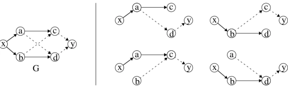
If shortest paths in the graph are not unique, the properties of locally shortest paths studied in Section 2 do not hold. Furthermore, using an arbitrary tie-breaking strategy may lead to incorrect results. Consider the example of Figure 3, where all edges have weight 1, and suppose that at some point the unique shortest paths of length 2 inP∗ are: hx, a, ci,hx, b, di,
ha, d, yi, and hb, c, yi. Notice that we can find no path of length 3 such that every subpath of length 2 is in P∗: therefore, no path of length 3 can be formed by update, leaving the
pair (x, y) incorrectly disconnected in P∗. In order update to be correct, we thus need a tie-breaking strategy that both ensures uniqueness and leads to a complete set of shortest paths closed under subpaths.
How can we break ties consistently? A first simple approach is to add some tiny random fraction to the weight of each edge: in this way, we can make the probability of finding two paths with the same weight arbitrarily small.
A more robust deterministic tie-breaking approach is the following. Without loss of generality, assume that V = {1,2, . . . , n}. We assign to each edge (u, v) a unique number ID(u, v) (e.g., ID(u, v) = u+nv), and for each path π we define ID(π) as the maximum ID of its edges. This allows us to define the extended weight ew(π) of a pathπ as follows. Definition 2 For any path π with at least one edge we define the extended weight of π as ew(π) =hw(π), ID(π)i, wherew(π)is the real weight ofπin the graph andID(π)is defined
x a b c d y x a c b c y x b d a d y x a c b c y x b d a d y G
Figure 3: If shortest paths are not unique, using an arbitrary tie-breaking strategy may lead to pairs of vertices connected in G, but disconnected in P∗. In this example, if P∗ contains
hx, a, ci, hx, b, di, ha, d, yi, and hb, c, yi as the unique shortest paths of length 2, then no locally shortest path between x and y can be obtained as the union of any two of them. as follows:
ID(π) =
(
u+nv if π =hu, vi
max{ ID(`(π)), ID(r(π))} otherwise
The extended weights of two pathsπ1 andπ2can be compared “lexicographically” in constant time by assuming that:
ew(π1)≤ew(π2) ⇔ w(π1)< w(π2) or
w(π1) =w(π2) and ID(π1)≤ID(π2)
We now show that using extended weights we can break ties consistently so that exactly one shortest path (if any) between each pair of vertices can be identified in a deterministic way. To do so, we define the following set of paths in a graph:
Definition 3 Let G be a graph with real-valued edge weights and let ew be the extended weight function of Definition 2. We define Sew as follows:
Sew ={ π ∈G : ∀πxy ⊆π, ∀π0xy ∈G, ew(πxy)≤ew(πxy0 ) }.
According to this definition, Sew contains every path that has minimum extended weight and whose subpaths have minimum extended weight as well (optimal-substructure property). As a consequence, Sew is closed under subpaths, i.e., every subpath of a path inSew belongs to Sew. It is easy to prove that there can be only one path in Sew between each pair of vertices.
Lemma 5 For each pair of vertices x and y in G, there can be at most one path πxy ∈ Sew connecting them.
Proof. The proof is by induction on the number of edges in the paths. The basis is trivially satisfied, since there can be only one path formed by one edge between each pair of vertices. Now, assume by induction that the claim holds for every path that uses at most k edges,
and suppose by contradiction that there are two different paths πxy ∈ Sew and πxy0 ∈ Sew that use at mostk+ 1 edges. Since their extended weights are equal, then bothπxy and πxy0 must contain the edge (u, v) such that ID(u, v) =ID(πxy) =ID(πxy0 ). Since every subpath of πxy and πxy0 belongs to Sew and uses at most k edges, then πxy and π0xy must have the same subpaths fromx tou and fromv toy. Thus, πxy and πxy0 must be equal, contradicting
the assumption that they are different. 2
Clearly, if πxy ∈ Sew, then πxy is a shortest path in G. We now show that, if there is a shortest path from x toy in G, then there must be a pathπxy ∈Sew.
Lemma 6 For each pair of connected vertices x and y in G, there is a path πxy ∈Sew.
Proof. Assume thaty is reachable from x in G, x6=y. Then, we show how to construct a pathπ∗
xy that satisfies Definition 3. We start with an empty πxy∗ and construct it one edge at the time. Let πxy be a path from x to y with minimum extended weight inG and let (u, v) be the edge with maximum ID inπxy, i.e., such that ID(u, v) = ID(πxy). We put (u, v) in π∗
xy and build recursively the subpathπ∗xuofπxy∗ ifx6=uand the subpathπvy∗ ofπxy∗ ifv 6=y. We now show that the above procedure constructs paths that belong to Sew. We prove this claim proceeding by induction on the path length. Letk be the number of edges inπ∗
xy. The base for k = 1 (π∗
xy = hx, yi) is trivial. Assume by induction that the claim holds for every path containing less thank edges and assume by contradiction that there is a subpath πab ∈π∗xy that is not of minimum extended weight. Three cases are possible:
(1) both vertices a and b are in π∗
xu; (2) both vertices a and b are in π∗
vy; (3) vertex a is in π∗
xu and vertex b is in π∗vy. Case (1) and (2) are not possible, since π∗
xu and π∗vy have strictly less than k edges, and thus by induction are in Sew. Assume that we are in case (3). Since πab is not of minimum extended weight, there must be a path π0
ab such that ew(πab0 ) < ew(πab). Note that, by construction π∗
xy contains only edges that lie on some shortest path from x to y in G, and thus w(πab) ≤ w(πab0 ). Consequently, it must be w(πab) = w(π0ab) and ID(πab0 ) < ID(πab). This implies that there is a shortest path fromxtoyavoiding edge (u, v), with an ID smaller than ID(u, v). This contradicts the fact that ID(u, v) is the ID of a path with minimum
extended weight from x toy. 2
By Lemma 5 and Lemma 6, Sew contains exactly one representative shortest path between each pair of vertices connected in G. Thus, we can conclude that |Sew| ≤ n2 and Sew is a complete set of unique shortest paths in G. For this reason, in the remainder of this paper we will assume that we can always ensure uniqueness of shortest paths by dealing with paths in Sew.
We now show that using the deterministic approach described above we can break ties consistently and ensure both completeness and uniqueness of shortest paths, avoiding in-consistencies like the one shown in Figure 3. As a matter of fact, we can easily modify the
code of the update operation given in Figure 2 so that at any time during a sequence of updates, P∗ =S
ew. Specifically, we keep an additional fieldID(π) for each path π stored in the data structure, and perform the following additional steps in fixupto maintain it as in Definition 2:
Line 4 ID(hu, vi)←u+nv Line 19 ID(πx0y)←max{ID(πx0b), ID(πxy) } Line 7 ID(hv, ui)←v+nu Line 23 ID(πxy0)←max{ID(πxy), ID(πay0) } Furthermore, we let the priority of any path π in P and H be ew(π). Thus, in line 11 and line 13 of fixup we pick paths with minimum ew, instead of minimum w. To check the correctness of this approach, we prove the following theorem.
Theorem 4 If we compare paths according to the extended weight function ew given in Definition 2, then P∗ =S
ew after each execution of update.
Proof. We first observe that for any path π, if edge weights in the graph are non-negative reals, the extended weight function ew given in Definition 2 satisfies the monotonic property ew(`(π)) ≤ ew(π) and ew(r(π)) ≤ ew(π). Moreover, by Lemma 5 and Lemma 6 there is exactly one path in Sew between each pair of connected vertices. Therefore, it is easy to check that Invariant 1 continues to hold if we compare paths according to ew instead of w: this implies that each path added toP∗ has minimum extended weight.
Furthermore, by construction, paths inP∗ are closed under subpaths, i.e., every subpath
of a path in P∗ is also inP∗: thus, P∗ =S
ew as in Definition 3. 2
We conclude this section by observing that each increase (resp. decrease) of an edge weight implies an increase (resp. decrease) of the corresponding extended weight. Furthermore, we notice that comparing extended weights still takes constant time. Thus, both Theorem 2 and Theorem 3 continue to hold using extended weights instead of the original weights in the graph.
4
Historical and Locally Historical Paths
Figure 4 shows a graph and a pathological fully dynamic update sequence such that each operation causes Θ(n3) changes in the set of locally shortest paths of the graph. This proves that maintaining locally shortest paths in a fully dynamic setting can require as much as Ω(n3) time per operation. To deal with fully dynamic update sequences efficiently, in this section we introduce other two classes of paths that we call historical paths and locally historical paths: historical paths will play the role of shortest paths, while locally historical paths will play the role of locally shortest paths. Unlike shortest paths and locally shortest paths, which only depend on the graph at a given time, these classes of paths capture the history of the changes in the graph, encompassing the time dimension of the problem. We define them as follows:
L1 40 30 10 L2 L3 L4 20
...
L1 40 30 L2 L3 L4Θ
(n)
20...
Θ
(n)
u
v
u
v
Figure 4: Pathological update sequence consisting of repeated deletion and re-insertion of edge (u, v). Each insertion/deletion causes Θ(n3) changes in the set of locally shortest paths. Locally shortest paths connecting vertices in layer L1 to vertices in layer L4 are highlighted as thick lines. Edges are directed from left to right and, unless explicitly shown, their weights are small values close to zero.
Definition 4 Let πxy be a path in G at time t, and let t0 ≤t be the time of the latest vertex update on πxy. We say that πxy is Historical at time t if it has been a shortest path at least once in the time interval [t0, t].
According to this definition, a shortest path is also a historical path. Although it may stop being a shortest path at some point, it keeps on being a historical path until a vertex update occurs on it.
Definition 5 We say that a path πxy is Locally Historical2 in G at time t if ei-ther:
(i) πxy consists of a single vertex, or
(ii) every proper subpath of πxy is a historical path in G at time t.
Unlike locally shortest paths, as defined in Definition 1, proper subpaths do not have to be shortest paths necessarily at the same time. Indeed, in a locally historical path, all proper subpaths have been shortest paths in the past; however, the path itself may have never been locally shortest.
The next lemma addresses the relationship between shortest paths, historical paths, and locally historical paths:
Lemma 7 If we denote by SP, HP, and LHP respectively the sets of shortest paths, his-torical paths, and locally hishis-torical paths in Gat any time in a sequence of updates, then the following inclusions hold at that time: SP ⊆HP ⊆LHP.
2In an earlier version of this paper, we used terminology potentially uniform paths instead of locally
HP SP LSP
LHP
Figure 5: Inclusions between shortest paths (SP), locally shortest paths (LSP), historical paths (HP), and locally historical paths (LHP).
Proof. The inclusionSP ⊆HP is straightforward from Definition 4. Let π be a historical path at time t and lett0 ≤t be the time of the latest vertex update on π. For every proper
subpath πb ⊂π, let bt≤t0 ≤t be the time of the latest vertex update onπ. By Definition 4,b
π has been a shortest path in the time interval [t0, t]. By the optimal-substructure property
of shortest paths, πb has been a shortest path in the time interval [t, t]b ⊇[t0, t], and thus it is
historical at time t. Consequently, HP ⊆LHP. 2
Figure 5 summarizes the relationship between shortest paths, locally shortest paths, historical paths, and locally historical paths. As we will see later on, the reason why we are considering locally historical paths is that they can be maintained very efficiently in a sequence of fully dynamic updates. Since by Lemma 7 locally historical paths include shortest paths, this implies that we can maintain information about dynamic shortest paths very efficiently. Historical paths, on the other hand, are only used as a tool for defining locally historical paths.
4.1
Properties of Locally Historical Paths
In this section we study combinatorial properties of locally historical paths, addressing their dependence on the number of historical paths in the graph. These properties will be crucial in Section 5 to designing our efficient algorithm for fully dynamic shortest paths. We start by analyzing the maximum number of paths that can be locally historical at each time during a sequence of updates.
Lemma 8 Let G be a graph subject to a sequence Σ of update operations. If at any time throughout the sequence Σ there are at most z historical paths between each pair of vertices and m edges in G, then at that time there can be at most zmn locally historical paths in G.
Proof. We follow the same argument given in the proof of Lemma 3. To build a locally historical path πxy = hx, u, . . . , yi, the first edge (x, u) can be chosen in m different ways, while the destination vertex y can be chosen among n different vertices. Since every proper subpath of πxy has to be historical and there are at most z historical paths between each
pair of vertices, there can be at most z historical subpaths between uand y. Thus there can
be at most zmn locally historical paths in G. 2
Another interesting question is how many locally historical paths can go through any given vertex in the graph. Since a path can stop being locally historical only when it is touched by a vertex update, this yields a worst-case bound on the number of paths that can stop being locally historical at each update. To address this, we first need to prove that, given any two distinct historical paths between any pair of vertices x and y, their latest updated vertices must be different.
Lemma 9 Let G be a graph subject to a sequence Σ of update operations and let x, y be any two vertices in G. If shortest paths are unique and we denote by σ(π) the latest vertex update on path π, then for any two distinct historical paths πxy and πxy0 in G at any time t, vσ(πxy) 6=vσ(π0xy).
Proof. Assume by contradiction that vσ(πxy) = vσ(π0xy), and thus tσ(πxy) = tσ(πxy0 ). By
Definition 4, both πxy and πxy0 have to be shortest paths at least once in the time interval [tσ(πxy), t], but this is impossible since neither of them is touched in the time interval (tσ(πxy), t],
and at each time there can be only one shortest path between x and y in G. 2 Lemma 10 Let G be a graph subject to a sequence Σ of update operations and let v be any vertex in G. If shortest paths are unique and at any time t throughout the sequence Σ there are at most z historical paths between each pair of vertices, then at time t there can be at most O(zn2) locally historical paths that contain v.
Proof. We first show that there can be at most O(zn2) locally historical paths having v as endpoint. Indeed, to form a locally historical path πvy = hv, x, . . . , yi, we can choose x andy in at mostO(n2) different ways; since every proper subpath ofπ
vy has to be historical and there are at mostz historical paths between each pair of vertices, there can be at most z historical subpaths between x and y. The argument for paths ending in v is completely analogous.
To complete the proof, it suffices to show that for each pair of vertices x, y, with x 6=v andy6=v, there can be at mostO(z) locally historical paths of the formhx, . . . , v, . . . , yi, i.e., havingv as an internal vertex. Denote by P the set of such paths, and let Q={π1, . . . , πq} be the subset ofP such that for eachπi ∈Q, v follows (or coincides with) vi inπi, where vi is the latest updated vertex in πi− {x, y}.
Consider now the set of subpaths Qb = {cπi = hx, . . . , vi, . . . , vi ⊂ πi, πi ∈ Q}. We first claim that|Q|=|Qb|. To prove this claim, we show that any two distinct paths πi and πj in
Q must give rise to distinct subpaths πbi ⊂ πi and πbj ⊂ πj in Q. Assume by contradictionb that this is not the case, i.e., πi 6=πj and πbi =πbj, which implies that vi =vj. Consider the subpaths ofπi and πj fromvi toy: those paths must be historical sinceπi and πj are locally historical and vi 6= x, and must share the same latest updated vertex, which can be either vi or y. By Lemma 9 they must be equal, which implies πi =πj, clearly a contradiction.
Thus, it must be|Q|=|Qb|. To conclude the proof of the lemma, suppose by contradiction that|P|>2z, and assume without loss of generality that |Q| ≥ |P|/2, and thus|Q|> z. By Definition 5, paths in Qb are historical at time t. Since |Q|=|Qb|> z, we can conclude that at timet there are more thanz historical paths between xandv inG, which contradicts the
assumptions of the lemma. 2
The next corollary, whose proof follows immediately from Definition 4, Definition 5, and Lemma 10, bounds the number of paths that stop being locally historical at each time during a sequence of updates:
Corollary 1 LetGbe a graph subject to a sequenceΣof update operations. If shortest paths are unique and at any time t throughout the sequenceΣ there are at most z historical paths between each pair of vertices, then the number of paths that stop being locally historical at each update is O(zn2) in the worst case.
We finally bound the number of paths that become locally historical at each time during a sequence of updates:
Theorem 5 Let G be a graph subject to a sequence Σ of update operations and let m be the maximum number of edges in G throughout sequence Σ. If shortest paths are unique and at any time throughout the sequenceΣ there are at most z historical paths between each pair of vertices, then the number of paths that become locally historical after each update is:
(1) O(zmn) in the worst case.
(2) O(zn2) amortized over Ω(m/n) update operations.
Proof. Analogous to the proof of Lemma 1. Indeed, Claim (1) follows immediately from Lemma 8. To prove Claim (2), we assign a debit to each locally historical path in the graph. The debit is paid for by the operation that makes it stop being locally historical. By Corollary 1, at most O(zn2) paths can stop being locally historical at each update. Moreover, by Lemma 8 there can be at most zmn locally historical paths in a graph at any time, so the total unpaid debit at the end of the sequence never exceeds zmn. Thus, the amortized number of paths that start being locally shortest after each update in any sequence of Ω(m/n) operations can be at most O(zn2). 2
4.2
A Worst-Case Scenario
We now show that there exists a graph and an update sequence that produces Ω(n3) historical paths. This implies by Theorem 5 an amortized number of Ω(n3) new locally historical paths per update. Consider the graph in Figure 6, whereL1. . . L6 are layers containingn/6 vertices each. The graphs induced by L1 ∪L2, L3 ∪L4 and L5 ∪L6 are complete bipartite graphs with edge weights equal to 1, while the graphs induced by L2∪L3 andL4∪L5 have weights shown below the corresponding edges. The update sequence is as follows:
L1 n
...
n+1 n+2 n+3 n+k n...
n-1 n-2 n-3 n-k L2 L3 L4 L5 L6 k+1=n/6Figure 6: Worst-case instance with Ω(n3) historical paths and an amortized number of Ω(n3) new locally historical paths per update.
Phase I. Perform the following sequence of k = (n/6)− 1 decreases on edges in L2∪L3: 1) n+ 1 → n−1 2) n+ 2 → n−2 3) n+ 3 → n−3 ... ... ... ... k) n+k → n−k
Phase II.Perform the following sequence of k = (n/6)− 1 increases on edges in L4∪L5: 1) n−k → n+k 2) n−(k−1) → n+ (k−1) 3) n−(k−2) → n+ (k−2) ... ... ... ... k) n−1 → n+ 1
During Phase I, (k+ 1)2 paths connecting L
1 toL5 become historical at each decrease, and thus at the end of Phase I there are Θ(k3) historical paths in total. During Phase II, at each increase, k paths connecting each pair of vertices in L1 and L6 become locally historical in the graph. Since k = (n/6)−1, each increase takes Ω(n3) time. Notice that this update sequence can be made arbitrarily long by repeating Phase I and Phase II back and forth many times.
The example considered here suggests that keeping too much information about the history of changes in a dynamic graph could be prohibitive, i.e., maintaining all the locally historical paths can lead to Ω(n3) time per update. In contrast, in the example considered in Figure 4 we have shown that keeping no information about the history of changes, i.e., keeping only locally shortest paths, can lead to cubic update times as well. In the next section we will discuss an effective compromise between those two extreme solutions.
4.3
Keeping Historical Paths Under Control: Smoothing
In this section, we show that it is possible to transform on-line every update sequence into another sequence so that the total number of historical paths in the graph is always very close to n2. To guarantee that this transformation does not alter the input update sequence by affecting the result of shortest path queries, we make sure that it produces exactly the same changes in the graph as the input sequence. In the following, we will call such a transformationSmoothing. Furthermore, we will calloptimala historical path that is also a shortest path.
We first observe that at any time t, if shortest paths are unique, then there can be at most n2 optimal historical paths. Any other historical path must have been optimal strictly before timet, and is no longer optimal at timet. By Definition 4, if we update a vertex, every non-optimal historical path containing it will immediately stop being historical. To become again historical, it has to be a shortest path once again. Therefore, to reduce the number of historical paths, it is sufficient to add to the input update sequence suitable operations whose only effect is to clean up non-optimal historical paths. For this reason, we will call these additional operationsCleanup Updates. To guarantee that cleanup updates do not alter the input update sequence by affecting the result of shortest path queries, we simply let them overwrite edge weights without changing their values. We now define how our smoothing strategy works:
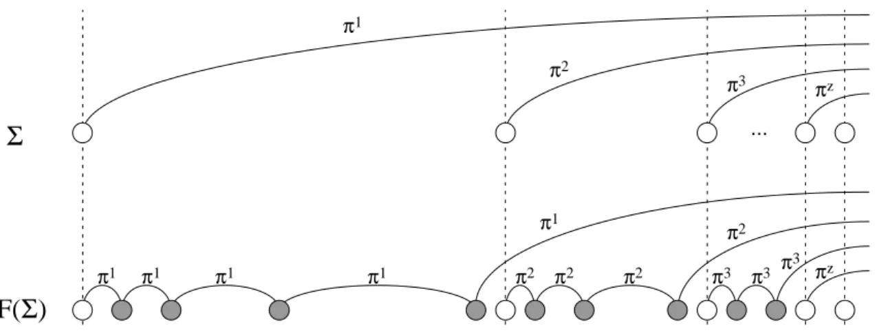
Definition 6 Let Σ = hσ1, σ2, . . . , σki be an update sequence and let F(Σ) =hσ1, δ11, . . . , δ q1 1 , σ2, δ21, . . . , δ q2 2 , . . . , σk, δ1k, . . . , δ qk k i
be another sequence derived from Σ such that each δij is a cleanup update, and such that, if a vertex is updated by operation σt in Σ, it is touched by cleanup update δij in F(Σ) when i = t+ 1, t+ 2, t+ 4, t+ 8, . . ., t + 2p, . . ., for some j. We call F(Σ) a Smoothed
Sequence derived from Σ, we refer to hδ1
i, . . . , δqiii as the Burst of Cleanup Updates
after σi, and we say that cleanup updateδtj+2p isTriggered by the Original Update
σt.
Note that a smoothed sequence is obtained by squeezing a burst of cleanup updates between each pair of consecutive updates in the original sequence. Throughout the paper, we assume that the burst of cleanup updates hδ1
i, . . . , δ qi
i i occurs exactly at the same time as update σi, i.e., tδj
i =tσi for any j. We now show that a smoothed sequence is operationally
equivalent to the sequence it is derived from, and produces a smaller number of historical paths.
Theorem 6 Let Σ = hσ1, σ2, . . . , σki be an update sequence of length k. Then the smoothed sequence F(Σ) =hσ1, δ11, . . . , δ q1 1 , σ2, δ21, . . . , δ q2 2 , . . . , σk, δ1k, . . . , δ qk k i of Definition 6 has the following properties:
πi πi+1 tσi tσi+1 tσi+T t
Σ
cleanup updates πi πi+1 πi πi πi tσi+T tσi+1 tF(
Σ
)
tσiFigure 7: Graphs of historical paths Hxy for an update sequence Σ and for the smoothed updated sequence F(Σ). If tσi+1 < tσi +T, then πi cannot be historical at time t in the
graph produced by F(Σ).
1. For 1≤i≤k, qi =O(logk);
2. For 1 ≤ i ≤ k, after performing operation σi, the graph produced by Σ and the graph produced by F(Σ) are equal;
3. At any time there are at mostO(logk) historical paths between each pair of vertices in the graph produced by F(Σ).
Proof. Properties 1 and 2 follow directly from Definition 6. To prove Property 3, we first note that a cleanup update on a vertex v does not create new historical paths: its only effect is to remove non-optimal historical paths containing vertexv. For each pair of vertices (x, y) in G, consider the graph of historical paths Hxy. There is a vertex in Hxy for each update operationτ inF(Σ) and there is an edge (τa, τb) in Hxy, with tτa < tτb, for each path πxy in
G having the following three properties:
(i) πxy contains bothvτa and vτb (possibly vτa =vτb);
(ii) no vertex in πxy is updated in the time interval (tτa, tτb);
(iii) πxy becomes a shortest path at some time t∈[tτa, tτb).
It is easy to see that at any time at most one path πxy in G can satisfy Properties (i), (ii) and (iii) above.
Let π1, . . . , πz be the historical paths between vertices xand y in the graph G obtained right after performing update σt in F(Σ), i.e., at time t. Let (τi,τbi) be the edge in Hxy corresponding to πi, 1 ≤i≤z. Since πi is historical at time t, it must be t
τi ≤t < tbτi. If τi
is a cleanup update, let σi be the original update that triggered τi, t
π1 π2 π3 πz ...
Σ
π1 π1 π1 π1 π1 π2 π2 π2 π2 π3 π3 π3 πzF(Σ)
Figure 8: Worst case instance of Σ such that at time k there are Θ(logk) historical paths between pair x, y in the graph produced byF(Σ).
historical pathπi we can associate an original updateσi, with t
σ1 < tσ2 < . . . < tσz ≤t. Let
σi and σi+1 be two such updates, and let T be the largest power of 2 smaller than t−t σi,
i.e., T = 2blog2(t−tσi)c. We claim that it must be t
σi+T ≤tσi+1.
Indeed, assume by contradiction thattσi+1 < tσi+T (see Figure 7). SinceT = 2blog2(t−tσi)c
is a power of 2, by Definition 6 there is a cleanup update triggered byσi that touches a vertex ofπiat time t
σi+T: thusπi cannot be historical at timetσi+T by Definition 4. Notice that,
since πi+1 must be a shortest path between xand y afterπi, and no vertex ofπi and πi+1 is updated in the time interval [tσi+1, t],πi cannot become again a shortest path between xand y in the time interval [tσi+1, t]. Thus πi cannot become historical again in the time interval [tσi+T, t], contradicting the assumption that πi was historical at timet.
We have thus shown that if π1, . . . , πz are historical paths at time t, there must be z updates σ1, . . . , σz in the original sequence Σ such that t
σi + 2blog2(t−tσi)c ≤ tσi+1 ≤ t, for 1≤i≤z−1. This implies z =O(logt) =O(logk). 2 We note that Θ(logk) historical paths between a pair of vertices in G can be actually realized, as illustrated in Figure 8.
5
Fully Dynamic Shortest Paths
In this section we show that the properties of locally historical paths given in Section 4 allow us to use the update algorithm of Section 3 in a fully dynamic setting, and to achieve O(ne 2) amortized time per update. This is the first general algorithm for fully dynamic all pairs shortest path that is faster than recomputing the solution from scratch after each update. The approach we follow here differs in just two points from Section 3:
Pxy set of locally historical paths from x toy in G P∗
xy set of historical paths from x to y inG
L(πxy) set of pre-extensions hx0, xi ·πxy of πxy that are locally historical paths in G L∗(π
xy) set of pre-extensions hx0, xi ·πxy of πxy that are historical paths in G
R(πxy) set of post-extensions πxy· hy, y0i of πxy that are locally historical paths in G R∗(π
xy) set of post-extensions πxy· hy, y0i of πxy that are historical paths in G Table 3: Notation introduced in Section 5.1.
1. We maintain locally historical paths instead of locally shortest paths. Since by Lemma 7 shortest paths are locally historical, this guarantees that we are still main-taining information about shortest paths.
2. We provide a new front-endfully-update for the update operation, which calls the update procedure of Figure 2, implementing the smoothing strategy of Section 4.3. We now describe in more detail how to achieve these modifications, and then discuss cor-rectness and time/space requirements of the new procedure fully-update.
5.1
Data Structure
We maintain exactly the same data structure described in Section 3.1, with just one differ-ence: we replace “shortest” with “historical”.
Pxy = {πxy : πxy is a locally historical path in G}
Pxy∗ = {πxy : πxy is a historical path in G}
L(πxy) = {πx0y =hx0, xi ·πxy : (x0, x)∈E and πx0y is a locally historical path inG} L∗(πxy) = {πx0y =hx0, xi ·πxy : (x0, x)∈E and πx0y is a historical path inG}
R(πxy) = {πxy0 =πxy · hy, y0i : (y, y0)∈E and πxy0 is a locally historical path inG } R∗(πxy) = {πxy0 =πxy · hy, y0i : (y, y0)∈E and πxy0 is a historical path in G}
In order to support the smoothing operation, we also keep for each vertexv the timetv of its latest update and a counter time of the number offully-update operations performed. The notation introduced in this section is summarized in Table 3.
5.2
Implementation of Operations
The operations are exactly the same as described in Section 3.2. The only difference is that we do not call directly the update procedure shown in Figure 2, but rather provide a new front-end procedure named fully-update and shown in Figure 9, which implements the smoothing strategy of Section 4.3 by calling the update procedure of Figure 2 for both original and cleanup updates.
5.3
Analysis
The correctness of query operations follows directly from Lemma 7. To prove the correctness of fully-update(v, w0), we observe that it calls update(v, w0) to update the data structure
after changing the weights of the edges incident to v to the new values w0 (line 3). Then, it
repeatedly calls update(v, w) on vertices that have to be smoothed (lines 4–5): notice that the call overwrites the edge weights without changing their values, and the only effect of this operation is to remove non-optimal historical paths from the data structure as discussed in Section 4.3. Therefore, it is sufficient to prove the correctness of update. To this aim, it is easy to check that both Invariant 1 and its proof continue to hold using the new data structure of Section 5.1 instead of the data structure of Section 3.1. We can thus prove the following theorem:
Theorem 7 If shortest paths are unique and edge weights are non-negative, then algorithm
update correctly updates Pxy and Pxy∗ for each pair of vertices x and y.
Proof. The proof is exactly the same as the proof of Theorem 2, provided that we suitably replace “shortest” with “historical” and “increase” with “update”. 2 We conclude our analysis of the fully dynamic algorithm by discussing time and space requirements of our implementation. To this aim, we first analyze procedure update in a fully dynamic setting.
Lemma 11 In a fully dynamic sequence of Ω(m/n) operations, if shortest paths are unique, edge weights are non-negative, and at any time there are at most z historical paths between each pair of vertices, our data structure supports each update operation in O(zn2logn) amortized time. The space used is O(zmn).
Proof. We rephrase the proof of Theorem 3, by suitably replacing “shortest” with “histor-ical”, and by using Lemma 10, Theorem 5, and Lemma 8 instead of Lemma 2, Theorem 1, and Lemma 3, respectively.
The bounds for queries are immediate, since the minimum weight path in the priority queue Pxy can be retrieved in optimal time.
Since each iteration of cleanup removes a path πxy from a constant number of lists and priority queues, it requires O(logn) time in the worst case. By Lemma 10, at most
fully-update(v, w0): 1. time←time+ 1 2. tv ←time
3. update(v, w0) {original update σ}
4. for each u∈V : time−tu = 2dlog2(time−tu)e do {smoothing}
5. update(u, w) {cleanup update δ} Figure 9: Implementation of the fully-update operation.
O(zn2) locally historical paths can go through the updated vertex in the worst case, and thus cleanup will perform at most O(zn2) iterations, thus spending at most O(zn2logn) time.
Next, it is easy to see thatPhase1 offixuprequiresO(nlogn) time in the worst case. To bound the time required byPhase 2 of fixup, we consider that finding the minimum in Pxy takes constant time and each insertion inH takesO(logn) time. This gives a total bound of O(n2logn) for this phase. Finally, we note that a path π
xy is a new locally historical path if and only if both`(πxy) =hx, . . . , bi ∈Pxb∗ andr(πxy) = ha, . . . , yi ∈Pay∗ afterthe update, and either`(πxy)6∈Pxb∗ orr(πxy)6∈Pay∗ before callingfixup. Thus, since inPhase 3 we process a shortest pathπxy extracted fromHonly if it was not already inPxy∗ before callingfixup, then we spend time only for the new locally historical paths. This implies thatPhase 3 requires O(n2logn) time for extracting theO(n2) pairs which are initially inH, plusO(logn) time to insert/delete each new locally historical path inHandP: letpthe number of such paths. By Theorem 5, there can be O(zn2) paths that start being locally historical after each update, amortized over a sequence of Ω(m/n) operations. Moreover, by Lemma 10, there can be at most O(zn2) locally historical paths that were removed by cleanup since they contain the updated vertex, and are added back by fixup: thus, p = O(zn2) and update requires O(zn2logn) overall time.
At any time, each locally historical path πxy can only appear in a constant number of data structures: namely, in H, Pxy, L(r(πxy)), R(`(πxy)), and possibly in Pxy∗ , L∗(r(πxy)), R∗(`(π
xy)). Thus, the space usage of our data structure is bounded by the number of locally historical paths in a graph, which is O(zmn) in the worst case by Lemma 8. 2 Theorem 8 In a fully dynamic sequence of Ω(m/n)operations, if shortest paths are unique and edge weights are non-negative, our data structure supports eachfully-update operation in O(n2log3
n) amortized time, and each distance and path query in optimal time. The space used is O(mnlogn).
Proof. As in the proof of Theorem 3, the bounds for queries are immediate. To prove our update bound, we observe that procedure fully-update generates the smoothed sequence of Definition 6: thus, by Theorem 6 at any time in a sequence ofk updates there are at most z =O(logk) historical paths between each pair of vertices in G.
By Lemma 11, each call to update requires O(n2lognlogk) amortized time. Since each
fully-update causes as many as O(logk) update operations, then the amortized running time of fully-update is O(n2lognlog2k) =O(n2log3n) on any sequence of lengthk, with k polynomial in n. To get rid of this assumption, we can simply restart our data structure from scratch every Θ(n2) operations. The space bound follows immediately from Lemma 11.