Research Article Robust Model Predictive Control of Networked Control Systems under Input Constraints and Packet Dropouts

(1)

Research Article

Robust Model Predictive Control of Networked Control Systems

under Input Constraints and Packet Dropouts

Deyin Yao,

1

Hamid Reza Karimi,

2

Yiyong Sun,

3

and Qing Lu

1 1_{College of Engineering, Bohai University, Jinzhou, Liaoning 121013, China}

2_{Department of Engineering, Faculty of Engineering and Science, University of Agder, 4898 Grimstad, Norway}

3_{Research Institute of Intelligent Control and Systems, Harbin Institute of Technology, Harbin, Heilongjiang 150080, China} Correspondence should be addressed to Deyin Yao; [email protected]

Received 22 May 2014; Accepted 4 June 2014; Published 16 July 2014 Academic Editor: Josep M. Rossell

Copyright © 2014 Deyin Yao et al. This is an open access article distributed under the Creative Commons Attribution License, which permits unrestricted use, distribution, and reproduction in any medium, provided the original work is properly cited. This paper deals with the problem of robust model predictive control (RMPC) for a class of linear time-varying systems with constraints and data losses. We take the polytopic uncertainties into account to describe the uncertain systems. First, we design a robust state observer by using the linear matrix inequality (LMI) constraints so that the original system state can be tracked. Second, the MPC gain is calculated by minimizing the upper bound of infinite horizon robust performance objective in terms of linear matrix inequality conditions. The method of robust MPC and state observer design is illustrated by a numerical example.

1. Introduction

Model predictive control (MPC) [1, 2] is an important method to handle control problems with systems having input, state, and output constraints [3–7]. Its current con-trol action is obtained by solving an online, at each time instant, open-loop constrained infinite horizon optimization problem. The current state of the system is treated as the initial state of optimal control problems [8], and only the first optimal control sequence is implemented [9]. In this line of the research, a model is used to predict the future behavior of the real system and obtain an optimal control sequence which satisfies the input, state, and output constraints. So the model quality is very vital in the robust MPC.

From such a viewpoint, it is a significant problem to develop the MPC algorithms, which are robust against model uncertainties, and guarantee a certain control performance objective [10–17]. The type of MPC has been studied for many years [18–21]. Recently, MPC is an efficient method in automatic control theory and industrial processes. In [22], a robust MPC is presented for a class of uncertain systems and then applied to angular positioning system. Besides, the robust MPC developed based on explicit model uncertainty descriptions has been proposed [23]. As one of

such descriptions, polytopic system model is considered to be an effective one for the uncertainty modeling of linear time-varying (LTV) systems.

With the increasing requirement of reliability, environ-mental sustainability, and profitability, we begin to apply the communication networks to the practical industrial process [24–31]. However, in the real systems, the measurement data may be transferred through multiple sensors. The sensors are connected to the controller via a network, which is shared by other networked control systems. Due to sensor aging and sensor temporal failure, the measured data may be transferred through many sensors in the real process via networks so that successive packet dropouts are unavoidable in the real industry process [32–34]. Moreover, another significant factor, input constraints, which stems from the restrictions of engineering equipment, cannot be ignored in industrial processes. Therefore, the robust MPC controller should be developed by considering packet dropouts and constraints.

In this paper, we describe an industrial process system as the linear time-varying system with packet dropouts from the MPC controller and dynamic output controller to the plant. Furthermore, a Bernoulli random binary distribution with known probabilities is used to describe the packet dropouts

Volume 2014, Article ID 478567, 11 pages http://dx.doi.org/10.1155/2014/478567

(2)

phenomena. Thus, the MPC controller can be analyzed and designed to guarantee that the closed-loop system is stochastically stable. Additionally, the Lyapunov function is adopted to handle the problem of designing the controller and state observer, which make the result less conservative. A numerical example is proposed to prove the effectiveness of the design method. The main merit of this paper is the following one: a robust MPC controller is developed for a control system with uncertainties, saturations, and packet dropouts under time-varying probabilities.

The organization of the paper is given as follows. The considered problem is denoted in Section 2. Section 3 for-mulates the infinite horizon robust performance objective. The procedure of obtaining the state observer gains is represented inSection 4. And the MPC controller gain and dynamic output controller are represented in Sections5and

6, respectively. We employ two numerical examples to certify the feasibility of the mentioned method inSection 7. Finally,

Section 8presents the conclusion.

Notation. The notation used in the paper is standard. The

superscript “𝑇” represents the matrix transposition andR𝑛𝑥

shows the 𝑛_𝑥-dimensional Euclidean space. And 𝐼 and 0 denote the identity matrix and zero matrix, respectively. The notations𝑃 > 0 and 𝑄 > 0mean that 𝑃and 𝑄are real symmetric and positive definite; the notation‖𝐴‖refers to the norm of matrix𝐴that is defined by‖𝐴‖ = √tr(𝐴𝑇𝐴), where “tr” stands for the trace operator.‖ ⋅ ‖₂ refers to the usual Euclidean vector norm. The symbol “∗” denotes the elements below the main diagonal of a symmetric block matrix. Prob{⋅}means the occurrence probability of the event

“⋅”.𝐸{𝑥}and𝐸{𝑥 | 𝑦}represent the expectation of event𝑥and

the expectation of𝑥conditional on𝑦, respectively.

2. Problem Formulation

First, we consider the linear time-varying system as follows:

𝑥 (𝑘 + 1) = 𝐴 (𝑘) 𝑥 (𝑘) + 𝐵 (𝑘) 𝑢 (𝑘) , 𝑦 (𝑘) = 𝐶𝑥 (𝑘) ,

[𝐴 (𝑘) 𝐵 (𝑘)] ∈ Ω,

(1)

where 𝑥(𝑘) ∈ R𝑛𝑥 _{is the plant state vector;}𝑦(𝑘) ∈ R𝑛𝑦 _is

the output of the plant;𝑢(𝑘) ∈R𝑛𝑢_{is the control input;}𝐴(𝑘)_, 𝐵(𝑘), and𝐶are system parameters.Ωis a given set. For the polytopic systems, the setΩis the polytope:

Ω =Co{[𝐴₁ 𝐵₁] , [𝐴₂ 𝐵₂] , . . . , [𝐴_𝐿 𝐵_𝐿]} , (2)

where Co represents the convex hull. Besides, if

[𝐴(𝑘) 𝐵(𝑘)] ∈ Ω, then for 𝜆_𝑖 ≥ 0, 𝑖 = 1, 2, . . . , 𝐿, and

∑𝐿_𝑖=1𝜆_𝑖 = 1, [𝐴(𝑘) 𝐵(𝑘)] = ∑_𝑖=1𝐿 𝜆_𝑖[𝐴_𝑖(𝑘) 𝐵_𝑖(𝑘)]. When

𝐿 = 1, it means that the system in (2) is becoming a linear

time-invariant system.

In this paper, the system matrices[𝐴(𝑘) 𝐵(𝑘)]are known clearly. However, the future matrices [𝐴(𝑘 + 𝑖) 𝐵(𝑘 + 𝑖)],

𝑖 ≥ 1, are indefinite but well known which change in a

given polytope setΩ. We assume that the linear discrete-time

system (1) has input constraints [35], which satisfies at each instant𝑘 ≥ 0, as follows:

‖𝑢 (𝑘 + 𝑖)‖₂≤ 𝑢_max, 𝑘, 𝑖 ≥ 0, (3)

where𝑢_maxrefers to the peak bound of the input𝑢.

In this paper, we consider a state observer to estimate the state of the plant (1) as follows:

̂𝑥 (𝑘 + 1) = 𝐴 (𝑘) ̂𝑥 (𝑘) + 𝐿 [𝑦 (𝑘) − 𝐶̂𝑥 (𝑘)] + 𝐵 (𝑘) 𝑢 (𝑘) , ̂𝑦 (𝑘) = 𝐶̂𝑥 (𝑘) ,

(4) where ̂𝑥(𝑘) ∈R𝑛𝑥 _{refers to the estimated state of}𝑥(𝑘)_and𝐿

refers to the state observer gain. It is assumed that the initial estimate state ̂𝑥₀ = ̂𝑥(0)and the initial output𝑦₀ = 𝑦(0) are known exactly. Note that system matrices[𝐴(𝑘) 𝐵(𝑘)], output𝑦(𝑘), and the estimated statê𝑥(𝑘), at each instant𝑘, are well known so that̂𝑥(𝑘+1)can be calculated by using (4). However, the estimated statê𝑥(𝑘 + 𝑖 + 1),𝑖 ≥ 1, is uncertain.

The MPC controller is to be determined as follows:

𝑢_𝑐(𝑘 + 𝑖 | 𝑘) = 𝐾 (𝑘) ̂𝑥 (𝑘 + 𝑖 | 𝑘) , 𝑖 ≥ 0, (5)

where 𝐾(𝑘)is the feedback control gain at time instant 𝑘. In MPC, only the first calculated control input𝑢_𝑐(𝑘 | 𝑘) =

𝐾̂𝑥(𝑘 | 𝑘)is complemented. At the next sampling time𝑘 + 1,

the statê𝑥(𝑘 + 1)is measured and𝐾is repeatedly computed by the optimization.

The form of dynamic output controller is as follows:

̂𝑥𝑐(𝑘 + 1) = 𝐴𝑐̂𝑥𝑐(𝑘) + 𝐵𝑐𝑦𝑐(𝑘) ,

𝑢_𝑐(𝑘) = 𝐶_𝑐̂𝑥𝑐(𝑘) ,

(6) where𝐴_𝑐, 𝐵_𝑐, and𝐶_𝑐are the unknown parameters of dynamic output controller.

Combining (1), (6), and (10), the augmented system is given as follows:

𝜃 (𝑘 + 1) = [𝐴 (𝑘) + ̂𝐴 (𝑘)] 𝜃 (𝑘) ,

𝑦 (𝑘) = 𝐶𝜃 (𝑘) , (7)

where𝜃(𝑘) = [𝑥𝑇(𝑘) ̂𝑥𝑇(𝑘)]𝑇,𝐶 = [𝐶 0], and

𝐴 (𝑘) = [𝐴 (𝑘) 𝛽𝐵 (𝑘) 𝐶𝑐

𝛼𝐵_𝑐𝐶 𝐴_𝑐 ] ,

̂

𝐴 (𝑘) = [ 0 𝛽 (𝑘) 𝐵 (𝑘) 𝐶̂ 𝑐

̂𝛼 (𝑘) 𝐵𝑐𝐶 0 ] .

(8)

In practical industrial processes, we have to not only consider the uncertainties in (2), but also consider a more important factor that is data loss. Data losses are inevitable in communication networks, because the measurement data may be transferred through many sensors in the real process. Here, we consider a stochastic variable𝛿(𝑘)to describe successive packet dropouts in a random way. The character-istic of the successive packet dropouts is the latest received

(3)

data that will be sent to the state observer. If the data is not updated, the control input will keep unchanged. More important is that taking the packet dropouts into account is consistent with the real situation design in industry. Therefore, signals transmitted through the communication network to the estimated state observer can be expressed as

𝑢 (𝑘) = 𝛿 (𝑘) 𝑢𝑐(𝑘) , (9)

where𝑢_𝑐(𝑘)is the control input that is computed by using the feedback gain𝐾(𝑘)which is determined at each instant

𝑘. 𝑢(𝑘) is the actual measurement signal of 𝑢_𝑐(𝑘) and transmitted to the plant (1) and state observer (4). We assume that the stochastic variable𝛿(𝑘)satisfies Prob{𝛿(𝑘) = 1} =

𝐸{𝛿(𝑘)} = 𝛿and Prob{𝛿(𝑘) = 0} = 1 − 𝛿. Let̃𝛿(𝑘) = 𝛿(𝑘) − 𝛿.

Then,𝐸{̃𝛿(𝑘)} = 0and𝐸{̃𝛿2(𝑘)} = 𝛿(1 − 𝛿) ≜ 𝜙2.

In a similar situation, we consider stochastic variables

𝛼(𝑘) and 𝛽(𝑘)to describe successive packet dropouts in a random way:

𝑢 (𝑘) = 𝛽 (𝑘) 𝑢𝑐(𝑘) ,

𝑦𝑐(𝑘) = 𝛼 (𝑘) 𝑦 (𝑘) ,

(10) where𝑢_𝑐(𝑘)is the control input,𝑢(𝑘)is the actual measure-ment signal of𝑢_𝑐(𝑘)which is transmitted to the plant (1), and

𝑦_𝑐(𝑘)is the actual signal of𝑦(𝑘)which is transmitted to the dynamic output controller, respectively. We assume that the stochastic variables𝛼(𝑘)and𝛽(𝑘)satisfy Prob{𝛼(𝑘) = 1} =

𝐸{𝛼(𝑘)} = 𝛼and Prob{𝛼(𝑘) = 0} = 1 − 𝛼and Prob{𝛽(𝑘) =

1} = 𝐸{𝛽(𝑘)} = 𝛽and Prob{𝛽(𝑘) = 0} = 1 − 𝛽, respectively.

Let̂𝛼(𝑘) = 𝛼(𝑘) − 𝛼and𝛽(𝑘) = 𝛽(𝑘) − 𝛽̂ , respectively. Then,

𝐸{̂𝛼(𝑘)} = 𝐸{ ̂𝛽(𝑘)} = 0, 𝐸{̂𝛼2(𝑘)} = 𝛼(1 − 𝛼) ≜ 𝑙2, and

𝐸{ ̂𝛽2_{(𝑘)} = 𝛽(1 − 𝛽) ≜ 𝑚}2_{, respectively.}

The following Lemma is used in the process of proof.

Lemma 1. Let𝐹and𝐺and𝐻and𝐸be the real matrices of

appropriate dimensions; then𝐹 + 𝐺𝐻𝐸 + 𝐸𝑇𝐻𝑇𝐺𝑇< 0if and

only if there exists a positive scalar𝜀 > 0 such that𝐹+𝜀−1𝐺𝐺𝑇+

𝜀𝐸𝑇_{𝐸 < 0} _{or, equivalently,}

[ [

𝐹 ∗ ∗

𝐺𝑇 _{−𝜀𝐼 0}

𝜀𝐸 0 −𝜀𝐼 ] ]

< 0. (11)

3. Infinite Horizon Robust Performance

Objective Analysis

In this paper, the aim of the robust MPC is to determine the model predictive control law{𝑢(𝑘 | 𝑘), 𝑢(𝑘 + 1 | 𝑘), . . . , 𝑢(𝑘 +

𝑖 | 𝑘)}, 𝑖 ≥ 1, which regulates the initial state of system

reaching the origin, making the robust performance objective minimum in the worst case and ensuring that the closed-loop system is asymptotically stable. In order to determine the control input𝑢(𝑘)under input constraints, we minimize the performance objective𝐽_∞(𝑘)through minimizing its upper bound. Consider the performance objective by minimizing the infinite horizon objective function𝐽_∞(𝑘)as follows:

min

𝑢(𝑘+𝑖|𝑘) [𝐴(𝑘+𝑖|𝑘) 𝐵(𝑘+𝑖|𝑘)]∈Ωmax 𝐽∞(𝑘) , (12)

where

𝐽_∞(𝑘) = 𝐸 {∑∞

𝑖=0

[𝑦𝑇(𝑘 + 𝑖 | 𝑘) 𝑅₁𝑦 (𝑘 + 𝑖 | 𝑘)

+𝑢𝑇(𝑘 + 𝑖𝑘) 𝑅₂𝑢 (𝑘 + 𝑖𝑘)] } ,

(13)

in which 𝑅₁ and 𝑅₂ are the positive-definite matrices that should be given firstly. It is worth noting that the choices of

𝑅₁and𝑅₂are unclear, which are usually adjusted according to the practical situation.

We consider transferring the minimization of𝐽_∞(𝑘)into minimizing its upper bound. Therefore, we assume that the following inequality holds for all𝑦(𝑘 | 𝑘),𝑢(𝑘 | 𝑘),𝑖 ≥ 0, satisfying the input constraints (3), and for any[𝐴(𝑘+𝑖) 𝐵(𝑘+

𝑖)] ∈ Ω,𝑖 ≥ 0:

𝐸 {𝑉 (̂𝑥 (𝑘 + 𝑖 + 1 | 𝑘)) | ̂𝑥 (𝑘 + 𝑖 | 𝑘)} − 𝑉 (̂𝑥 (𝑘 + 𝑖 | 𝑘))

≤ −𝐸 {𝑦𝑇(𝑘 + 𝑖 | 𝑘) 𝑅₁𝑦 (𝑘 + 𝑖 | 𝑘)

+ 𝑢𝑇(𝑘 + 𝑖 | 𝑘) 𝑅2𝑢 (𝑘 + 𝑖 | 𝑘)} ,

(14)

where 𝑉(̂𝑥(𝑘)) = ̂𝑥𝑇(𝑘)𝑃̂𝑥(𝑘)and 𝑃 > 0 is a symmetric matrix.

Proof. Firstly, we construct a Lyapunov function𝑉(̂𝑥(𝑘)) =

̂𝑥𝑇_{(𝑘)𝑃̂𝑥(𝑘)}_{, where}_{𝑃 > 0}_{is a symmetric matrix. We assume}

that𝐸{𝑉(̂𝑥(∞ | 𝑘))} = 0. By summing (14) from𝑖 = 0to

𝑖 = ∞, we can obtain the following inequality:

max

[𝐴(𝑘+𝑖) 𝐵(𝑘+𝑖)]∈Ω,𝑖≥0𝐽∞(𝑘) ≤ 𝑉 (̂𝑥 (𝑘 | 𝑘))

− 𝐸 {𝑉 (̂𝑥 (∞ | 𝑘))} ≤ ̂𝑥𝑇(𝑘 | 𝑘) 𝑃̂𝑥 (𝑘 | 𝑘) .

(15)

Let𝛾be the upper bound of𝐽_∞(𝑘)and we have the following inequality:

̂𝑥𝑇(𝑘 | 𝑘) 𝑃̂𝑥 (𝑘 | 𝑘) ≤ 𝛾. (16)

In a similar situation, we consider transferring the minimiza-tion of𝐽_∞(𝑘)into minimizing its upper bound. Therefore, we assume that the following inequality holds for all𝑦(𝑘 | 𝑘),

𝑢(𝑘 | 𝑘),𝑖 ≥ 0, satisfying the input constraints (3), and for

any[𝐴(𝑘 + 𝑖) 𝐵(𝑘 + 𝑖)] ∈ Ω,𝑖 ≥ 0:

𝐸 {𝑉 (𝜃 (𝑘 + 𝑖 + 1 | 𝑘)) | 𝜃 (𝑘 + 𝑖 | 𝑘)} − 𝑉 (𝜃 (𝑘 + 𝑖 | 𝑘))

≤ −𝐸 {𝑦𝑇(𝑘 + 𝑖 | 𝑘) 𝑅₁𝑦 (𝑘 + 𝑖 | 𝑘)

+ 𝑢𝑇(𝑘 + 𝑖 | 𝑘) 𝑅₂𝑢 (𝑘 + 𝑖 | 𝑘)} .

(4)

4. State Observer Design

In this section, we consider the design of state observer. The form of state observer is (4). Therefore, the state estimation error is𝑒(𝑘) = 𝑥(𝑘) − ̂𝑥(𝑘). Combining (1) with (4), we can derive the error dynamics as follows:

𝑒 (𝑘 + 1) = (𝐴 − 𝐿𝐶) 𝑒 (𝑘) . (18)

Next we use LMI to determine the state observer gain𝐿. First, we should construct a Lyapunov functioñ𝑉(𝑒(𝑘))as follows:

̃

𝑉 (𝑒 (𝑘)) = 𝑒𝑇(𝑘) ̃𝑃𝑒 (𝑘) , ̃𝑃 > 0. (19)

We assume that the Lyapunov functioñ𝑉(𝑒(𝑘))satisfies the following inequality:

̃

𝑉 (𝑒 (𝑘 + 1)) − 𝜌2̃𝑉 (𝑒 (𝑘)) < −𝑒𝑇(𝑘) ̃𝐿𝑒 (𝑘) , (20)

where𝜌 (0 < 𝜌 < 1)is a decay rate and̃𝐿 ≥ 0is a weighting matrix which are determined by the designer. According to the assumption (20), the state observer gain𝐿can be obtained by the following theorem.

Theorem 2. If there exist ̃𝑃 > 0and𝑄 = ̃𝑃𝐿̃ , one can derive

the following inequality:

[ 𝜌_{̃𝑃𝐴 − ̃𝑄𝐶 ̃𝑃] > 0,}2̃𝑃 − ̃𝐿 ∗ (21)

where the state observer gain is derived by𝐿 = ̃𝑃−1𝑄̃.

Therefore, the estimated state ̂𝑥can track the original system

states𝑥and̂𝑥(𝑘) → 𝑥(𝑘)when𝑘 → ∞.

Proof. Inequality (20) is equivalent to

𝜌2̃𝑃 − ̃𝐿 − Π𝑇(𝑘) ̃𝑃Π (𝑘) > 0, (22)

whereΠ(𝑘) = 𝐴(𝑘) − 𝐿𝐶. However, inequality (22) can be converted into the following form:

𝜌2̃𝑃 − ̃𝐿 − (̃𝑃Π (𝑘))𝑇̃𝑃−1(̃𝑃Π (𝑘)) > 0. (23)

By using Schur complement, we can obtain the following LMI constraint:

[𝜌_{̃𝑃Π (𝑘) ̃𝑃] > 0.}2̃𝑃 − ̃𝐿 ∗ (24)

Let𝑄 = ̃𝑃𝐿̃ ; inequality (24) is equivalent to

[ 𝜌_{̃𝑃𝐴 (𝑘) − ̃𝑄𝐶 ̃𝑃] > 0.}2̃𝑃 − ̃𝐿 ∗ (25)

It is established for all [𝐴(𝑘) 𝐵(𝑘)] ∈ Ω. And the state observer gain𝐿is obtained by𝐿 = ̃𝑃−1𝑄̃.

5. MPC Controller Design

Now our goal is to design a robust MPC to generate an optimal control law so that the performance objective can be achieved. In the following,Theorem 3is given to guarantee that the desired performance objective can be implemented by computing𝐾(𝑘)in (5) for linear discrete-time systems (1) under constraints (3) and packet dropouts (9). We can obtain the following theorem.

Theorem 3. Assume that the uncertainty Ω is a prescribed

polytope and the probabilities𝛿take values from0to1. The

control input(5)under a series of constrained input (3)that

minimizes𝐽_∞(𝑘)is obtained by

𝐾 = 𝑌𝑄−1, (26)

where𝑄 > 0is symmetric and the upper bound𝛾of𝐽_∞(𝑘)can

be solved by the following minimization problem:

min

𝑢(𝑘|𝑘),𝑄,𝑌 𝛾 (27)

subject to

[ 1 ̂𝑥_∗ 𝑇(𝑘 | 𝑘)_𝑄 ] ≥ 0, (28)

[ [ [ [ [ [ [ [ [ [ [ [ [ [ [ [ [

−𝑄 0 Γ 𝑌𝑇𝐵𝑇 _𝑌𝑇_𝑅1/2

2 𝑄𝑇𝐶𝑇𝑅1/21 𝑄𝑇𝐶𝑇 0

∗ −Λ 0 0 0 0 𝑄𝑇_𝐶𝑇 ₀

∗ ∗ −𝑄 0 0 0 0 𝐿

∗ ∗ ∗ −𝑄_𝜙₂ 0 0 0 0

∗ ∗ ∗ ∗ −𝛾𝐼

𝛿2+ 𝜙2 0 0 0

∗ ∗ ∗ ∗ ∗ −𝛾𝐼 0 0

∗ ∗ ∗ ∗ ∗ ∗ −𝜀𝐼 0

∗ ∗ ∗ ∗ ∗ ∗ ∗ −𝜀𝐼

] ] ] ] ] ] ] ] ] ] ] ] ] ] ] ] ]

< 0,

[𝑢2max𝐼 𝑌

∗ 𝑄] ≥ 0,

(5)

where𝐿 = 𝜀𝐿and𝜀 > 0is a positive scalar andΓ = 𝑄𝑇𝐴 +

𝛿𝑌𝑇_𝐵𝑇_.

At each future time instant, there exists the optimal control law to minimize the performance objective. Finally, the closed-loop system will be asymptotically stable.

Proof. In order to achieve the robust MPC performance

objective under input constraint and packet dropouts, there exist three LMIs that need to be feasible. The first LMI is obtained by (16); by minimizing the upper bound of 𝛾, we can get the second LMI; the third LMI is obtained by solving the input constraint (3). In the following, we give the proof.

Let𝑄 = 𝛾𝑃−1 > 0and use Schur complement we can

obtain inequality (28). Combining (4), (5), and (9) with (14), we have

𝐸 {̂𝑥𝑇(𝑘 + 𝑖 | 𝑘) [(𝐴 − 𝐿𝐶)𝑇𝑃 (𝐴 − 𝐿𝐶)

+ 𝛿(𝐴 − 𝐿𝐶)𝑇𝑃𝐵𝐾

+ 𝛿𝐾𝑇𝐵𝑇𝑃 (𝐴 − 𝐿𝐶)

+ (𝛿2+ 𝜙2) 𝐾𝑇𝐵𝑇𝑃𝐵𝐾

+ 𝐶𝑇𝑅₁𝐶 + (𝛿2+ 𝜙2) 𝐾𝑇𝑅₂𝐾 − 𝑃]

× ̂𝑥 (𝑘 + 𝑖 | 𝑘) + ̂𝑥𝑇(𝑘 + 𝑖 | 𝑘) [(𝐴 − 𝐿𝐶)𝑇𝑃𝐿𝐶

+𝛿𝐾𝑇𝐵𝑇𝑃𝐿𝐶]

× 𝑥 (𝑘 + 𝑖 | 𝑘) + 𝑥𝑇(𝑘 + 𝑖 | 𝑘) [𝐶𝑇𝐿𝑇𝑃 (𝐴 − 𝐿𝐶)

+𝛿𝐶𝑇𝐿𝑇𝑃𝐵𝐾]

×̂𝑥 (𝑘 + 𝑖 | 𝑘) + 𝑥𝑇(𝑘 + 𝑖 | 𝑘) 𝐶𝑇𝐿𝑇𝑃𝐿𝐶𝑥 (𝑘 + 𝑖 | 𝑘) }

< 0.

(30) Since𝑄 = 𝛾𝑃−1, inequality (30) is equivalent to

𝐸 {̂𝑥𝑇(𝑘 + 𝑖 | 𝑘) [(𝐴 − 𝐿𝐶)𝑇𝑄−1(𝐴 − 𝐿𝐶)

+ 𝛿(𝐴 − 𝐿𝐶)𝑇𝑄−1𝐵𝐾

+ 𝛿𝐾𝑇𝐵𝑇𝑄−1(𝐴 − 𝐿𝐶)

+ (𝛿2+ 𝜙2) 𝐾𝑇𝐵𝑇𝑄−1𝐵𝐾

+ 𝛾−1𝐶𝑇𝑅1𝐶

+ (𝛿2+ 𝜙2) 𝛾−1𝐾𝑇𝑅₂𝐾 − 𝑄−1]

× ̂𝑥 (𝑘 + 𝑖 | 𝑘) + ̂𝑥𝑇(𝑘 + 𝑖 | 𝑘) [ (𝐴 − 𝐿𝐶)𝑇𝑄−1𝐿𝐶

+ 𝛿𝐾𝑇𝐵𝑇𝑄−1𝐿𝐶]

× 𝑥 (𝑘 + 𝑖 | 𝑘) + 𝑥𝑇(𝑘 + 𝑖 | 𝑘)

× [𝐶𝑇𝐿𝑇𝑄−1(𝐴 − 𝐿𝐶) + 𝛿𝐶𝑇𝐿𝑇𝑄−1𝐵𝐾] ̂𝑥 (𝑘 + 𝑖 | 𝑘)

+𝑥𝑇_{(𝑘 + 𝑖 | 𝑘) 𝐶}𝑇_𝐿𝑇_𝑄−1_{𝐿𝐶𝑥 (𝑘 + 𝑖 | 𝑘) }}

< 0,

(31) by pre-multiplying and post-multiplying (31) by𝑄𝑇 and𝑄, respectively. And (31) is satisfied if there exists a weighting positive-definite matrixΛsuch that

𝐸 {𝑄𝑇_{̂𝑥𝑇_{(𝑘 + 𝑖 | 𝑘) [(𝐴 − 𝐿𝐶)}𝑇_𝑄−1_{(𝐴 − 𝐿𝐶)}

+ 𝛿(𝐴 − 𝐿𝐶)𝑇_𝑄−1_𝐵𝐾

+ 𝛾−1𝐶𝑇𝑅₁𝐶

+ (𝛿2+ 𝜙2) 𝛾−1𝐾𝑇𝑅₂𝐾 − 𝑄−1]

× ̂𝑥 (𝑘 + 𝑖 | 𝑘) + ̂𝑥𝑇(𝑘 + 𝑖 | 𝑘)

× [(𝐴 − 𝐿𝐶)𝑇𝑄−1𝐿𝐶 + 𝛿𝐾𝑇𝐵𝑇𝑄−1𝐿𝐶]

× 𝑥 (𝑘 + 𝑖 | 𝑘) + 𝑥𝑇(𝑘 + 𝑖 | 𝑘)

× [𝐶𝑇𝐿𝑇𝑄−1(𝐴 − 𝐿𝐶) + 𝛿𝐶𝑇𝐿𝑇𝑄−1𝐵𝐾] ̂𝑥 (𝑘 + 𝑖 | 𝑘)

+𝑥𝑇(𝑘 + 𝑖𝑘) [𝐶𝑇𝐿𝑇𝑄−1𝐿𝐶 − Λ] 𝑥 (𝑘 + 𝑖 | 𝑘) } 𝑄}

< 0.

(32) Inequality (32) is equivalent to

𝐸{_{

{

𝜃𝑇_{(𝑘 + 𝑖 | 𝑘) [}

[

𝑄𝑇_Φ𝑄 _𝑄𝑇_Ψ𝑇_𝑄−1_𝐿𝐶𝑄

𝑄𝑇𝐶𝑇𝐿𝑇𝑄−1Ψ𝑄 𝑄𝑇𝐶𝑇𝐿𝑇𝑄−1𝐿𝐶𝑄 − Λ

] ]

× 𝜃 (𝑘 + 𝑖 | 𝑘)}_}

} < 0,

(6)

where

Φ = (𝐴 − 𝐿𝐶)𝑇𝑄−1(𝐴 − 𝐿𝐶)

+ 𝛿 (𝐴 − 𝐿𝐶)𝑇𝑄−1𝐵𝐾

+ 𝛾−1𝐶𝑇𝑅1𝐶 + (𝛿2+ 𝜙2) 𝛾−1𝐾𝑇𝑅2𝐾 − 𝑄−1,

Ψ = 𝐴 − 𝐿𝐶 + 𝛿𝐵𝐾,

𝜃 (𝑘 + 𝑖 | 𝑘) = [̂𝑥𝑇(𝑘 + 𝑖 | 𝑘)𝑥𝑇(𝑘 + 𝑖 | 𝑘)]𝑇.

(34) Inequality (33) is equivalent to

[ [

𝑄𝑇Φ𝑄 𝑄𝑇[(𝐴 − 𝐿𝐶 + 𝛿𝐵𝐾) 𝑄−1𝐿𝐶] 𝑄

𝑄𝑇_𝐶𝑇_𝐿𝑇_𝑄−1_{(𝐴 − 𝐿𝐶 + 𝛿𝐵𝐾) 𝑄} _𝑄𝑇_𝐶𝑇_𝐿𝑇_𝑄−1_{𝐿𝐶𝑄 − Λ} ]

]

< 0. (35)

By using Schur complement repeatedly andLemma 1, we can obtain the following inequality:

[ [ [ [ [ [ [ [ [ [ [ [ [ [ [ [ [

−𝑄 0 𝑄𝑇𝐴 + 𝛿𝑌𝑇𝐵𝑇 𝑌𝑇𝐵𝑇 𝑌𝑇𝑅1/2₂ 𝑄𝑇𝐶𝑇𝑅1/2₁ 𝑄𝑇𝐶𝑇 0

∗ −Λ 0 0 0 0 𝑄𝑇_𝐶𝑇 ₀

∗ ∗ −𝑄 0 0 0 0 𝐿

∗ ∗ ∗ −𝑄_𝜙₂ 0 0 0 0

∗ ∗ ∗ ∗ −𝛾𝐼

𝛿2+ 𝜙2 0 0 0

∗ ∗ ∗ ∗ ∗ −𝛾𝐼 0 0

∗ ∗ ∗ ∗ ∗ ∗ −𝜀𝐼 0

∗ ∗ ∗ ∗ ∗ ∗ ∗ −𝜀𝐼

] ] ] ] ] ] ] ] ] ] ] ] ] ] ] ] ]

< 0, (36)

where𝑌 = 𝐾 𝑄and𝐿 = 𝜀𝐿and𝜀 > 0is a positive scalar. Combining (3), (5), (9), (16), and (26), we have

max

𝑖≥0 ‖𝑢(𝑘 + 𝑖 | 𝑘)‖

2 2

≤max

𝑖≥0 󵄩󵄩󵄩󵄩𝑢𝑐(𝑘 + 𝑖 | 𝑘)󵄩󵄩󵄩󵄩

2 2

=max

𝑖≥0 󵄩󵄩󵄩󵄩󵄩𝑌𝑄 −1

̂𝑥(𝑘 + 𝑖 | 𝑘)󵄩󵄩󵄩󵄩󵄩22

≤max

𝑖≥0 󵄩󵄩󵄩󵄩󵄩𝑌𝑄

−1/2_𝑄−1/2

̂𝑥(𝑘 + 𝑖 | 𝑘)󵄩󵄩󵄩󵄩󵄩22

= 𝜆_max(𝑄−1/2𝑌𝑇𝑌𝑄−1/2) ≤ 𝑢2_max.

(37)

By using Schur complement, we can obtain

[ [

𝑢2

max𝐼 ∗

𝑌𝑇 _𝑄]

]

≥ 0. (38)

6. Dynamic Output Controller

Theorem 4. Assume that the uncertaintyΩ is a prescribed

polytope and the probabilities𝛼and𝛽take values from0to1.

The control input(5)under a series of constrained inputs(3)

that minimizes𝐽_∞(𝑘)is obtained by

𝐴_𝑐 = 𝐺₁𝑊₂−1,

𝐵_𝑐 = ̃𝐵𝐶−1,

𝐶_𝑐 = 𝐺₂𝑊₂−1,

(39)

where𝑊₂ > 0is symmetric and the upper bound𝛾of𝐽_∞(𝑘)

can be solved by the following minimization problem:

min

𝑢(𝑘|𝑘),𝑄,𝑌 𝛾 (40)

subject to

[ 1 𝜃_∗ 𝑇(𝑘 | 𝑘)_𝑊 ] > 0, (41)

[Υ1 Υ2

∗ Υ₃] > 0, (42)

[𝑊 𝐺̃2𝑇

∗ 𝑢2

max𝐼] ≥ 0, (43)

(7)

Υ1=

[ [ [ [ [ [ [ [ [ [ [ [ [ [

−𝑊1 0 𝑊1𝑇𝐴𝑇 0 0 0 𝑊1𝑇𝐶𝑇𝑅1/21 0

∗ −𝑊₂ 𝛽𝐺𝑇

2𝐵𝑇 𝐺𝑇1 𝑞𝐺𝑇2𝐵𝑇 0 0 𝑊2𝑇𝐶𝑇𝑐𝑅1/22

∗ ∗ −𝑊₁ 0 0 0 0 0

∗ ∗ ∗ −𝑊₂ 0 0 0 0

∗ ∗ ∗ ∗ −𝑊₁ 0 0 0

∗ ∗ ∗ ∗ ∗ −𝑊₂ 0 0

∗ ∗ ∗ ∗ ∗ ∗ −𝛾𝐼 0

∗ ∗ ∗ ∗ ∗ ∗ ∗ −𝛾𝐼_𝑆

] ] ] ] ] ] ] ] ] ] ] ] ] ]

, (44)

Υ2= [

[

𝐶𝑊₁ 0 0 0 0 0 0 0

0 0 0 𝛼 ̃𝐵𝑇 _{0 𝑙 ̃𝐵}𝑇 _{0 0}]

]

𝑇

, Υ3= [−𝜀𝐼 0_{∗ −𝜀𝐼] ,} (45)

𝐴_𝑐 = 𝐺₁𝑊−1

2 ,𝐵𝑐 = ̃𝐵𝐶−1,𝐶𝑐 = 𝐺2𝑊2−1,𝜀 > 0is a positive

scalar, and𝐺̃₂= [0 𝐺₂].

Proof. Let𝑊 = 𝛾𝑃−1 > 0and, using Schur complement, we

can obtain inequality (41). Combining (10) and (7) with (18), we have

𝐸 {𝜃𝑇(𝑘 + 𝑖 | 𝑘) [𝐴𝑇(𝑘) 𝑃𝐴 (𝑘) + ̂𝐴𝑇(𝑘) 𝑃 ̂𝐴 (𝑘)

−𝑃 + ̃𝐶𝑇𝑅₁𝐶 + 𝑠̃̃ 𝐶𝑇_𝑐𝑅₂𝐶̃_𝑐] 𝜃 (𝑘 + 𝑖𝑘) }

< 0,

(46)

by premultiplying and postmultiplying (46) by𝑊𝑇and𝑊, respectively. By further transformation, we can achieve

− 𝑊 + 𝑊 + 𝑊𝑇𝐵𝑇𝑊−1𝐵𝑊 + 𝑊𝑇𝐶̃𝑇(𝛾𝑅−1₁ ) ̃𝐶𝑊

+ 𝑠𝑊𝑇𝐶̃𝑇_𝑐 (𝛾𝑅−1₂ ) ̃𝐶_𝑐𝑊 < 0, (47)

where 𝐵 = [ 0 𝑚𝐵𝐶𝑐

𝑙𝐵𝑐𝐶 0 ],𝐶̃𝑐 = [0 𝐶𝑐], 𝑊 = 𝑊𝑇_𝐴𝑇_(𝑘)𝑊−1_𝐴(𝑘)_{, and} _{𝑠 = 𝛽}2 _{+ 𝑚}2_{. By using Schur}

complement repeatedly and Lemma 1, we can obtain the following inequality:

[ [ [ [ [ [ [ [ [ [ [ [ [ [ [ [ [ [

−𝑊1 0 𝑊1𝑇𝐴𝑇 0 0 0 𝑊̂ 0 𝑊1𝑇𝐶𝑇 0

∗ −𝑊₂ 𝛽𝐺𝑇

2𝐵𝑇 𝐺𝑇1 ̌𝐺 0 0 𝑊̌ 0 0

∗ ∗ −𝑊₁ 0 0 0 0 0 0 0

∗ ∗ ∗ −𝑊₂ 0 0 0 0 0 𝛼 ̃𝐵

∗ ∗ ∗ ∗ −𝑊₁ 0 0 0 0 0

∗ ∗ ∗ ∗ ∗ −𝑊2 0 0 0 𝑙 ̃𝐵

∗ ∗ ∗ ∗ ∗ ∗ −𝛾𝐼 0 0 0

∗ ∗ ∗ ∗ ∗ ∗ ∗ −𝛾𝐼_𝑆 0 0

∗ ∗ ∗ ∗ ∗ ∗ ∗ ∗ −𝜀𝐼 0

∗ ∗ ∗ ∗ ∗ ∗ ∗ ∗ ∗ −𝜀𝐼

] ] ] ] ] ] ] ] ] ] ] ] ] ] ] ] ] ]

> 0, (48)

where𝑊 = 𝑊̂ ₁𝑇𝐶𝑇𝑅1/2₁ , ̌𝐺 = 𝑞𝐺𝑇₂𝐵𝑇,𝑊 = 𝑊̌ ₂𝑇𝐶𝑇_𝑐𝑅1/2₂ , and

𝜀 > 0is a positive scalar.

7. Simulation Results

Consider the following uncertain polytope system:

𝐴₁= [0.01942_{−0.5100 0.02000] ,}0

𝐴₂= [0.01942_{−0.5100 0.01000] ,}0

𝐵₁= 𝐵₂= 𝐵 = [1 −0.0787]𝑇,

𝐶₁= 𝐶₂= 𝐶 = [1 −0.4] ,

𝐷₁= 𝐷₂= 𝐷 = 0,

(49)

where the polytope formed by the two local discrete models is as follows:

(8)

0 20 40 60 80 100 −0.025

−0.02 −0.015 −0.01 −0.005 0 0.005 0.01 0.015 0.02

Time (s) x1

x2

St

at

e r

es

p

o

n

se

o

f c

los

ed-lo

o

p

syst

em

Figure 1: The state response of closed-loop system.

In the simulation, let[𝐴(𝑘) 𝐵(𝑘)] = [𝐴₁ 𝐵]. The input con-straint is as follows:

|𝑢 (𝑘)| ≤ 0.25, 𝑘 ≥ 0. (51)

InTheorem 2, the𝐿_𝐷𝑖decay rate𝜌and weighting matrix̃𝐿are given as

𝜌2= 0.8, ̃𝐿 = [0.1 0_{0 0.1] .} (52)

Then, the infinite horizon robust performance objective

𝐽_∞(𝑘)has the following weighting matrices:𝑅₁ = 0.01, 𝑅₂ =

0.00001.

Another weighting matrixΛis given as

Λ = [0.01 0_{0 0.1] ,} (53)

where the initial states of the real system (1) and the state observer are𝑥₀= [0.02 0]𝑇and̂𝑥₀= [0.02 −0.01]𝑇, respec-tively.

The state observer gain𝐿and MPC controller gain𝐾are obtained as𝐿 = [0.0167 − 0.4458]𝑇 and𝐾= [−0.7147

0.4889], respectively.

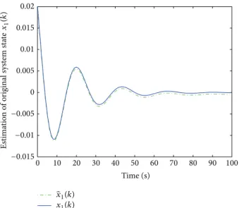
In Figure 1, the two curves are the state of the original closed-loop system. The solid line represents the real state

𝑥_𝑖(𝑘)(𝑖 = 1, 2) of the original closed-loop system and the

dashed line denotes its estimated state ̂𝑥_𝑖(𝑘) (𝑖 = 1, 2), respectively, in Figures 2 and 3. In Figure 4, the curve denotes the control input𝑢(𝑘)under the robust performance objective with the constrained input. The curve shows the output of closed-loop system, which converges to zero when

𝑘 → ∞inFigure 5.

0 10 20 30 40 50 60 70 80 90 100

−0.015 −0.01 −0.005 0 0.005 0.01 0.015 0.02

Time (s)

Es

tima

tio

n

o

f o

riginal syst

em st

at

e

x1

(k

)

̂x1(k)

x1(k)

Figure 2: Estimation of original system state𝑥₁(𝑘).

0 20 40 60 80 100

Time (s)

Estima

tio

n

o

f o

riginal syst

em st

at

e

x2

(k

)

x2(k)

̂x2(k)

−0.03 −0.025 −0.02 −0.015 −0.01 −0.005 0 0.005 0.01 0.015

Figure 3: Estimation of original system state𝑥₂(𝑘).

−0.02 −0.015 −0.01 −0.005 0.01 0.005

Time (s)

u(

k)

0

0 20 40 60 80 100

(9)

0 0.02 0.015 0.01 0.005

−0.005 −0.01

y(

k)

Time (s)

0 20 40 60 80 100

Figure 5: The output of closed-loop system.

Consider the following uncertain polytope system:

𝐴₁= [0.04942 −0.01₀ _{0.03000] ,}

𝐴₂= [0.04942 −0.01₀ _{0.01000] ,}

𝐵₁= 𝐵₂= 𝐵 = [−0.43 0]𝑇,

𝐶₁= 𝐶₂= 𝐶 = [1 0.4] ,

𝐷₁= 𝐷₂= 𝐷 = 0,

(54)

where the polytope formed by the two local discrete models is as follows:

[𝐴 (𝑘) 𝐵 (𝑘)] ∈ Ω =Co{[𝐴₁ 𝐵] , [𝐴₂ 𝐵]} . (55)

In the simulation, let [𝐴(𝑘) 𝐵(𝑘)] = [𝐴₁ 𝐵]. The input constraint is as follows:

|𝑢 (𝑘)| ≤ 0.2, 𝑘 ≥ 0. (56)

Then, the infinite horizon robust performance objective

𝐽_∞(𝑘)has the following weighting matrices:

𝑅₁= 1, 𝑅₂= 0.8, (57)

where the initial states of the real system (1) and the dynamic output controller are𝑥₀= [0 − 0.00001]𝑇and̂𝑥_𝑐= [0.35 −

0.09]𝑇, respectively.

The dynamic output controller gains,𝐴_𝑐, 𝐵_𝑐, and𝐶_𝑐, are obtained as

𝐴_𝑐= [−0.4597 −0.0821_{0.1933 −0.2124] ,}

𝐵_𝑐= [0.3845_{0.1024] ,}

𝐶_𝑐= [−0.0187 0.0850] .

(58)

0 5 10 15 20 25 30 35 40 45 50

−5 −4 −3 −2 −1 4 3 2 1 0

×10−5

Time (s)

x1

x2

St

at

e r

es

p

o

n

se

o

f o

p

en-lo

o

p

syst

em

Figure 6: The state response of open-loop system.

0 10 20 30 40 50

Time (s)

x3

x4

×10−3

7 6 5 4 3 2 1 0 −1

St

at

e r

es

p

o

n

se

o

f c

los

ed-lo

o

p

syst

em

Figure 7: The state response of closed-loop system.

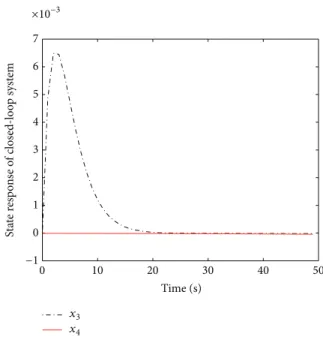
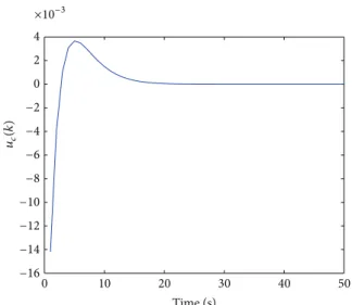
InFigure 6, the two curves are the state of the original open-loop system. InFigure 7, the two curves are the state of the original closed-loop system. InFigure 8, the two curves are the state of the dynamic output controller. The curve denotes the control input𝑢(𝑘)under the robust performance objective with the constrained input inFigure 9. The curve represents the control output𝑢_𝑐(𝑘)of dynamic output con-troller inFigure 10. The curve shows the output of closed-loop system, which converges to zero when𝑘 → ∞inFigure 11.

8. Conclusion

In this paper, we have designed an output-feedback MPC to solve the problem of the robust MPC with input constraints and successive packet dropouts. The method makes use of

(10)

0 0.05 0.1 0.15 0.2 0.25 0.3 0.35

St

at

e r

es

p

o

n

se

o

f d

yna

mic o

u

tp

u

t co

n

tr

o

ller

̂x1

̂x2

0 10 20 30 40 50

Time (s) −0.1

−0.05

Figure 8: The state response of dynamic output controller.

0 10 20 30 40 50

Time (s)

×10−3

u(

k)

−12 −10 −8 −6 −4 −2 0 2 4

Figure 9: The control input signal𝑢(𝑘).

infinite horizon min-max algorithm with LMI constraints. First, we have constructed a state observer. Then, the opti-mization problem can be solved by dealing with some LMI constraints. We can obtain the control input sequence by dealing with the infinite horizon robust MPC and input constraint based on the estimated state of observer. From the simulation, the design method of robust MPC with input constraint has been verified feasiblely. As a future work, we will develop the output-feedback MPC algorithm combined with nonlinear MPC and its optimization.

Conflict of Interests

The authors declare that there is no conflict of interests regarding the publication of this paper.

×10−3

−12 −14 −16 −10 −8 −6 −4 −2 0 2 4

uc

(k

)

0 10 20 30 40 50

Time (s)

Figure 10: The control output signal 𝑢_𝑐(𝑘) of dynamic output controller.

×10−3

0 10 20 30 40 50

Time (s)

y(

k)

7 6 5 4 3 2 1 0 −1

Figure 11: The output of closed-loop system.

References

[1] E. F. Camacho and C. B. Alba, Model Predictive Control, Springer, 2013.

[2] P. J. Campo and M. Morari, “Robust model predictive control,” inProceedings of the American Control Conference, pp. 1021– 1026, IEEE, 1987.

[3] R. Yang, G. Liu, P. Shi, C. Thomas, and M. V. Basin, “Predictive output feedback control for networked control systems,”IEEE Transactions on Industrial Electronics, vol. 61, no. 1, pp. 512–520, 2014.

[4] D. Q. Mayne, J. B. Rawlings, C. V. Rao, and P. O. M. Scokaert, “Constrained model predictive control: stability and optimal-ity,”Automatica, vol. 36, no. 6, pp. 789–814, 2000.

[5] Y. Xia, H. Yang, P. Shi, and M. Fu, “Constrained infinite-horizon model predictive control for fuzzy-discrete-time systems,”IEEE Transactions on Fuzzy Systems, vol. 18, no. 2, pp. 429–436, 2010.

(11)

[6] A. Casavola, M. Giannelli, and E. Mosca, “Min-max predictive control strategies for input-saturated polytopic uncertain sys-tems,”Automatica, vol. 36, no. 1, pp. 125–133, 2000.

[7] J. H. Lee and Z. Yu, “Worst-case formulations of model predic-tive control for systems with bounded parameters,”Automatica, vol. 33, no. 5, pp. 763–781, 1997.

[8] S. Yin, H. Luo, and S. X. Ding, “Real-time implementation of fault-tolerant control systems with performance optimization,” IEEE Transactions on Industrial Electronics, vol. 61, no. 5, pp. 2402–2411, 2013.

[9] S. Rakovic,Robust control of constrained discrete time systems: characterization and implementation [Ph.D. thesis], Imperial College London, University of London, 2005.

[10] H. R. Karimi, “Robust 𝐻_∞filter design for uncertain linear systems over network with network-induced delays and output quantization,”Modeling, Identification and Control, vol. 30, no. 1, pp. 27–37, 2009.

[11] S. Yin, S. X. Ding, A. Haghani, H. Hao, and P. Zhang, “A comparison study of basic data-driven fault diagnosis and process monitoring methods on the benchmark Tennessee Eastman process,”Journal of Process Control, vol. 22, no. 9, pp. 1567–1581, 2012.

[12] S. Yin, S. X. Ding, A. H. A. Sari, and H. Hao, “Data-driven monitoring for stochastic systems and its application on batch process,”International Journal of Systems Science, vol. 44, no. 7, pp. 1366–1376, 2013.

[13] H. Li, X. Jing, H.-K. Lam, and P. Shi, “Fuzzy sampled-data control for uncertain vehicle suspension systems,”IEEE Trans-actions on Cybernetics, vol. 44, no. 7, pp. 1111–1126, 2014. [14] H. Li, H. Liu, H. Gao, and P. Shi, “Reliable fuzzy control for

active suspension systems with actuator delay and fault,”IEEE Transactions on Fuzzy Systems, vol. 20, no. 2, pp. 342–357, 2012. [15] H. Li, X. Jing, and H. R. Karimi, “Output-feedback-based H_∞ control for vehicle suspension systems with control delay,”IEEE Transactions on Industrial Electronics, vol. 61, no. 1, pp. 436–446, 2014.

[16] H. Li, J. Yu, C. Hilton, and H. Liu, “Adaptive sliding-mode control for nonlinear active suspension vehicle systems using T-S fuzzy approach,”IEEE Transactions on Industrial Electronics, vol. 60, no. 8, pp. 3328–3338, 2013.

[17] H. Li, H. Gao, P. Shi, and X. Zhao, “Fault-tolerant control of Markovian jump stochastic systems via the augmented sliding mode observer approach,”Automatica, 2014.

[18] F. A. Cuzzola, J. C. Geromel, and M. Morari, “An improved approach for constrained robust model predictive control,” Automatica, vol. 38, no. 8, pp. 1183–1189, 2002.

[19] S. J. Qin and T. A. Badgwell, “A survey of industrial model predictive control technology,”Control Engineering Practice, vol. 11, no. 7, pp. 733–764, 2003.

[20] Y. J. Wang and J. B. Rawlings, “A new robust model predictive control method I: theory and computation,”Journal of Process Control, vol. 14, no. 3, pp. 231–247, 2004.

[21] P. J. Campo and M. Morari, “∞-norm formulation of model predictive control problems,” inProceedings of the IEEE Amer-ican Contro Conference, pp. 339–343, Seattle, Wash, USA, June 1986.

[22] M. V. Kothare, V. Balakrishnan, and M. Morari, “Robust con-strained model predictive control using linear matrix inequali-ties,”Automatica, vol. 32, no. 10, pp. 1361–1379, 1996.

[23] Z. Wan and M. V. Kothare, “Robust output feedback model predictive control using off-line linear matrix inequalities,” Journal of Process Control, vol. 12, no. 7, pp. 763–774, 2002.

[24] H. Gao and T. Chen, “Network-based 𝐻_∞ output tracking control,”IEEE Transactions on Automatic Control, vol. 53, no. 3, pp. 655–667, 2008.

[25] Y. Zhao, H. Gao, J. Lam, and B. Du, “Stability and stabilization of delayed T-S fuzzy systems: a delay partitioning approach,”IEEE Transactions on Fuzzy Systems, vol. 17, no. 4, pp. 750–762, 2009. [26] H. R. Karimi, N. A. Duffie, and S. Dashkovskiy, “Local capacity𝐻_∞ control for production networks of autonomous work systems with time-varying delays,”IEEE Transactions on Automation Science and Engineering, vol. 7, no. 4, pp. 849–857, 2010.

[27] H. R. Karimi, “Delay-range-dependent linear matrix inequality approach to quantized 𝐻_∞ control of linear systems with network-induced delays and norm-bounded uncertainties,” Proceedings of the Institution of Mechanical Engineers I: Journal of Systems and Control Engineering, vol. 224, no. 6, pp. 689–700, 2010.

[28] R. Yang, P. Shi, G. P. Liu, and H. Gao, “Network-based feedback control for systems with mixed delays based on quantization and dropout compensation,” Automatica, vol. 47, no. 12, pp. 2805–2809, 2011.

[29] H. Gao and T. Chen, “Stabilization of nonlinear systems under variable sampling: a fuzzy control approach,”IEEE Transactions on Fuzzy Systems, vol. 15, no. 5, pp. 972–983, 2007.

[30] H. Gao, Y. Zhao, J. Lam, and K. Chen, “H_𝑏𝑚∞fuzzy filtering of nonlinear systems with intermittent measurements,”IEEE Transactions on Fuzzy Systems, vol. 17, no. 2, pp. 291–300, 2009. [31] T. Chai, L. Zhao, J. Qiu, F. Liu, and J. Fan, “Integrated network-based model predictive control for setpoints compensation in industrial processes,”IEEE Transactions on Industrial Informat-ics, vol. 9, no. 1, pp. 417–426, 2013.

[32] J. Zhang, Y. Xia, and P. Shi, “Design and stability analysis of networked predictive control systems,”IEEE Transactions on Control Systems Technology, vol. 21, no. 4, pp. 1495–1501, 2013. [33] S. Sun, “Linear optimal state and input estimators for networked

control systems with multiple packet dropouts,”International Journal of Innovative Computing, Information and Control, vol. 8, no. 10, pp. 7289–7305, 2012.

[34] D. Q. Mayne, S. V. Rakovi´c, R. Findeisen, and F. Allg¨ower, “Robust output feedback model predictive control of con-strained linear systems: time varying case,”Automatica, vol. 45, no. 9, pp. 2082–2087, 2009.

[35] R. Moitie, M. Quincampoix, and V. M. Veliov, “Optimal control of discrete-time uncertain systems with imperfect measurement,”Institute of Electrical and Electronics Engineers: Transactions on Automatic Control, vol. 47, no. 11, pp. 1909–1914, 2002.

(12)

Submit your manuscripts at

http://www.hindawi.com

Hindawi Publishing Corporation

http://www.hindawi.com Volume 2014

Mathematics

Journal of

Mathematical Problems in Engineering

Hindawi Publishing Corporation http://www.hindawi.com

Differential Equations International Journal of

Volume 2014

http://www.hindawi.com Volume 2014 Hindawi Publishing Corporationhttp://www.hindawi.com Volume 2014

http://www.hindawi.com Volume 2014 Mathematical PhysicsAdvances in

Complex Analysis

Journal of

Optimization

Journal of

Combinatorics

http://www.hindawi.com Volume 2014 International Journal of

Journal of Hindawi Publishing Corporation

Function Spaces

Abstract and Applied Analysis Hindawi Publishing Corporation

International Journal of Mathematics and Mathematical Sciences

Hindawi Publishing Corporation http://www.hindawi.com Volume 2014

The Scientific

World Journal

Discrete Dynamics in Nature and Society Hindawi Publishing Corporation

Discrete Mathematics

Journal of

http://www.hindawi.com Volume 2014 Hindawi Publishing Corporationhttp://www.hindawi.com Volume 2014

Research Article Robust Model Predictive Control of Networked Control Systems under Input Constraints and Packet Dropouts