Department of Mathematical Sciences University of Massachusetts Lowell
Applied and
Preface xxiii
I
Preliminaries
1
1 Introduction 1
1.1 Chapter Summary . . . 1
1.2 Overview of this Course . . . 1
1.3 Solving Systems of Linear Equations . . . 2
1.4 Imposing Constraints . . . 2
1.5 Operators . . . 2
1.6 Acceleration . . . 3
2 An Overview of Applications 5 2.1 Chapter Summary . . . 6
2.2 Transmission Tomography . . . 6
2.2.1 Brief Description . . . 6
2.2.2 The Theoretical Problem . . . 7
2.2.3 The Practical Problem . . . 7
2.2.4 The Discretized Problem . . . 8
2.2.5 Mathematical Tools . . . 8
2.3 Emission Tomography . . . 8
2.3.1 Coincidence-Detection PET . . . 9
2.3.2 Single-Photon Emission Tomography . . . 9
2.3.3 The Line-Integral Model for PET and SPECT . . . 10
2.3.4 Problems with the Line-Integral Model . . . 10
2.3.5 The Stochastic Model: Discrete Poisson Emitters . . 11
2.3.6 Reconstruction as Parameter Estimation . . . 11
2.3.7 X-Ray Fluorescence Computed Tomography . . . 12
2.4 Magnetic Resonance Imaging . . . 12
2.4.1 Alignment . . . 13
2.4.2 Precession . . . 13
2.4.3 Slice Isolation . . . 13
2.4.4 Tipping . . . 13
2.4.5 Imaging . . . 14
2.4.6 The Line-Integral Approach . . . 14
2.4.7 Phase Encoding . . . 14
2.4.8 A New Application . . . 14
2.5 Intensity Modulated Radiation Therapy . . . 15
2.5.1 Brief Description . . . 15
2.5.2 The Problem and the Constraints . . . 15
2.5.3 Convex Feasibility and IMRT . . . 15
2.6 Array Processing . . . 16
2.7 A Word about Prior Information . . . 17
3 A Little Matrix Theory 21 3.1 Chapter Summary . . . 21
3.2 Vector Spaces . . . 22
3.3 Matrix Algebra . . . 24
3.3.1 Matrix Operations . . . 24
3.3.2 Matrix Inverses . . . 25
3.3.3 The Sherman-Morrison-Woodbury Identity . . . 26
3.4 Bases and Dimension . . . 27
3.4.1 Linear Independence and Bases . . . 27
3.4.2 Dimension . . . 29
3.4.3 Rank of a Matrix . . . 30
3.5 Representing a Linear Transformation . . . 31
3.6 The Geometry of Euclidean Space . . . 32
3.6.1 Dot Products . . . 32
3.6.2 Cauchy’s Inequality . . . 34
3.7 Vectorization of a Matrix . . . 34
3.8 Solving Systems of Linear Equations . . . 35
3.8.1 Row-Reduction . . . 35
3.8.2 Row Operations as Matrix Multiplications . . . 37
3.8.3 Determinants . . . 37
3.8.4 Sylvester’s Nullity Theorem . . . 38
3.8.5 Homogeneous Systems of Linear Equations . . . 39
3.8.6 Real and Complex Systems of Linear Equations . . . 41
3.9 Under-Determined Systems of Linear Equations . . . 41
3.10 Over-Determined Systems of Linear Equations . . . 43
4 The ART, MART and EM-MART 45 4.1 Chapter Summary . . . 45
4.2 Overview . . . 45
4.3 The ART in Tomography . . . 46
4.4.1 Simplifying the Notation . . . 49
4.4.2 Consistency . . . 49
4.4.3 WhenAx=bHas Solutions . . . 49
4.4.4 WhenAx=bHas No Solutions . . . 50
4.4.5 The Geometric Least-Squares Solution . . . 50
4.5 The MART . . . 51
4.5.1 A Special Case of MART . . . 51
4.5.2 The MART in the General Case . . . 52
4.5.3 Cross-Entropy . . . 53
4.5.4 Convergence of MART . . . 53
4.6 The EM-MART . . . 54
II
Algebra
59
5 More Matrix Theory 61 5.1 Chapter Summary . . . 615.2 Proof By Induction . . . 62
5.3 Schur’s Lemma . . . 63
5.4 Eigenvalues and Eigenvectors . . . 65
5.4.1 The Hermitian Case . . . 67
5.5 The Singular Value Decomposition (SVD) . . . 69
5.5.1 Defining the SVD . . . 69
5.5.2 An Application in Space Exploration . . . 71
5.5.3 A Theorem on Real Normal Matrices . . . 72
5.5.4 The Golub-Kahan Algorithm . . . 73
5.6 Generalized Inverses . . . 74
5.6.1 The Moore-Penrose Pseudo-Inverse . . . 74
5.6.2 An Example of the MP Pseudo-Inverse . . . 75
5.6.3 Characterizing the MP Pseudo-Inverse . . . 75
5.6.4 Calculating the MP Pseudo-Inverse . . . 75
5.7 Principal-Component Analysis and the SVD . . . 76
5.7.1 An Example . . . 77
5.7.2 DecomposingD†D . . . 77
5.7.3 DecomposingD Itself . . . 78
5.7.4 Using the SVD in PCA . . . 78
5.8 The PCA and Factor Analysis . . . 78
5.9 The MUSIC Method . . . 79
5.10 Singular Values of Sparse Matrices . . . 80
5.11 The “Matrix Inversion Theorem” . . . 83
5.12 Matrix Diagonalization and Systems of Linear ODE’s . . . 83
6 Metric Spaces and Norms 89
6.1 Chapter Summary . . . 90
6.2 Metric Space Topology . . . 90
6.2.1 General Topology . . . 90
6.2.2 Metric Spaces . . . 91
6.3 Analysis in Metric Space . . . 91
6.4 Motivating Norms . . . 93
6.5 Norms . . . 94
6.5.1 Some Common Norms on CJ . . . . 95
6.5.1.1 The 1-norm . . . 95
6.5.1.2 The∞-norm . . . 95
6.5.1.3 Thep-norm . . . 95
6.5.1.4 The 2-norm . . . 95
6.5.1.5 Weighted 2-norms . . . 95
6.6 The H¨older and Minkowski Inequalities . . . 96
6.6.1 H¨older’s Inequality . . . 96
6.6.2 Minkowski’s Inequality . . . 97
6.7 Matrix Norms . . . 98
6.7.1 Induced Matrix Norms . . . 98
6.7.2 Some Examples of Induced Matrix Norms . . . 100
6.7.3 The Two-Norm of a Matrix . . . 101
6.7.4 The Two-norm of an Hermitian Matrix . . . 102
6.7.5 Thep-norm of a Matrix . . . 103
6.7.6 Diagonalizable Matrices . . . 104
6.8 Estimating Eigenvalues . . . 105
6.8.1 Using the Trace . . . 106
6.8.2 Gerschgorin’s Theorem . . . 106
6.8.3 Strictly Diagonally Dominant Matrices . . . 106
6.9 Conditioning . . . 107
6.9.1 Condition Number of a Square Matrix . . . 107
7 Under-Determined Systems of Linear Equations 109 7.1 Chapter Summary . . . 109
7.2 Minimum Two-Norm Solutions . . . 110
7.3 Minimum Weighted Two-Norm Solutions . . . 110
7.4 Minimum One-Norm Solutions . . . 111
7.5 Sparse Solutions . . . 112
7.5.1 Maximally Sparse Solutions . . . 112
7.5.2 Why the One-Norm? . . . 112
7.5.3 Comparison with the Weighted Two-Norm Solution 113 7.5.4 Iterative Reweighting . . . 113
7.6.1 Signal Analysis . . . 114
7.6.2 Locally Constant Signals . . . 115
7.6.3 Tomographic Imaging . . . 116
7.7 Positive Linear Systems . . . 117
7.8 Feasible-Point Methods . . . 117
7.8.1 The Reduced Newton-Raphson Method . . . 117
7.8.1.1 An Example . . . 118
7.8.2 A Primal-Dual Approach . . . 119
8 Convex Sets 121 8.1 Chapter Summary . . . 121
8.2 A Bit of Topology . . . 121
8.3 Convex Sets inRJ . . . 123
8.3.1 Basic Definitions . . . 123
8.3.2 Orthogonal Projection onto Convex Sets . . . 125
8.4 Geometric Interpretations ofRJ . . . 127
8.5 Some Results on Projections . . . 129
9 Linear Inequalities 131 9.1 Chapter Summary . . . 131
9.2 Theorems of the Alternative . . . 132
9.2.1 A Theorem of the Alternative . . . 132
9.2.2 More Theorems of the Alternative . . . 132
9.2.3 Another Proof of Farkas’ Lemma . . . 135
9.3 Linear Programming . . . 137
9.3.1 An Example . . . 137
9.3.2 Canonical and Standard Forms . . . 137
9.3.3 Weak Duality . . . 138
9.3.4 Strong Duality . . . 139
III
Algorithms
141
10 Fixed-Point Methods 143 10.1 Chapter Summary . . . 14410.2 Operators . . . 144
10.3 Contractions . . . 145
10.3.1 Lipschitz Continuity . . . 145
10.3.1.1 An Example: Bounded Derivative . . . 145
10.3.1.2 Another Example: Lipschitz Gradients . . . 145
10.3.2 Non-expansive Operators . . . 145
10.3.4 Eventual Strict Contractions . . . 147
10.3.5 Instability . . . 149
10.4 Gradient Descent . . . 149
10.4.1 Using Sequential Unconstrained Minimization . . . . 149
10.4.2 Proving Convergence . . . 150
10.4.3 An Example: Least Squares . . . 151
10.5 Two Useful Identities . . . 151
10.6 Orthogonal Projection Operators . . . 152
10.6.1 Properties of the OperatorPC . . . 152
10.6.1.1 PC is Non-expansive . . . 153
10.6.1.2 PC is Firmly Non-expansive . . . 153
10.6.1.3 The Search for Other Properties of PC . . 154
10.7 Averaged Operators . . . 154
10.7.1 Gradient Operators . . . 157
10.7.2 The Krasnoselskii-Mann Theorem . . . 157
10.8 Affine Linear Operators . . . 158
10.8.1 The Hermitian Case . . . 158
10.8.2 Example: Landweber’s Algorithm . . . 160
10.8.3 What ifB is not Hermitian? . . . 160
10.9 Paracontractive Operators . . . 160
10.9.1 Diagonalizable Linear Operators . . . 161
10.9.2 Linear and Affine Paracontractions . . . 163
10.9.3 The Elsner-Koltracht-Neumann Theorem . . . 163
10.10Applications of the KM Theorem . . . 165
10.10.1 The ART . . . 165
10.10.2 The CQ Algorithm . . . 165
10.10.3 Landweber’s Algorithm . . . 166
10.10.4 Projected Landweber’s Algorithm . . . 167
10.10.5 Successive Orthogonal Projection . . . 167
11 Jacobi and Gauss-Seidel Methods 169 11.1 Chapter Summary . . . 169
11.2 The Jacobi and Gauss-Seidel Methods: An Example . . . . 170
11.3 Splitting Methods . . . 170
11.4 Some Examples of Splitting Methods . . . 172
11.5 Jacobi’s Algorithm and JOR . . . 173
11.5.1 The JOR in the Nonnegative-definite Case . . . 174
11.6 The Gauss-Seidel Algorithm and SOR . . . 175
11.6.1 The Nonnegative-Definite Case . . . 175
11.6.2 The GS Algorithm as ART . . . 176
11.6.3 Successive Overrelaxation . . . 177
11.6.4 The SOR for Nonnegative-DefiniteQ. . . 178
12 A Tale of Two Algorithms 181
12.1 Chapter Summary . . . 181
12.2 Notation . . . 182
12.3 The Two Algorithms . . . 182
12.4 Background . . . 182
12.5 The Kullback-Leibler Distance . . . 183
12.6 The Alternating Minimization Paradigm . . . 184
12.6.1 Some Pythagorean Identities Involving the KL Dis-tance . . . 184
12.6.2 Convergence of the SMART and EMML . . . 185
12.7 Sequential Optimization . . . 187
12.7.1 Sequential Unconstrained Optimization . . . 187
12.7.2 An Example . . . 187
12.7.3 The SMART Algorithm . . . 188
12.7.4 The EMML Algorithm . . . 188
13 Block-Iterative Methods I 189 13.1 Chapter Summary . . . 189
13.2 Recalling the MART Algorithm . . . 189
13.3 The EMML and the SMART Algorithms . . . 190
13.3.1 The EMML Algorithm . . . 190
13.3.2 The SMART Algorithm . . . 190
13.4 Block-Iterative Methods . . . 191
13.4.1 Block-Iterative SMART . . . 191
13.4.2 Seeking a Block-Iterative EMML . . . 191
13.4.3 The BI-EMML Algorithm . . . 192
13.4.4 The EMART Algorithm . . . 193
13.5 KL Projections . . . 193
13.6 Some Open Questions . . . 194
14 The Split Feasibility Problem 195 14.1 Chapter Summary . . . 195
14.2 The CQ Algorithm . . . 195
14.3 Particular Cases of the CQ Algorithm . . . 196
14.3.1 The Landweber algorithm . . . 196
14.3.2 The Projected Landweber Algorithm . . . 197
14.3.3 Convergence of the Landweber Algorithms . . . 197
14.3.4 The Simultaneous ART (SART) . . . 197
14.3.5 Application of theCQAlgorithm in Dynamic ET . 198 14.3.6 More on the CQ Algorithm . . . 199
14.4 Applications of the PLW Algorithm . . . 199
15 Conjugate-Direction Methods 201 15.1 Chapter Summary . . . 201
15.2 Iterative Minimization . . . 201
15.3 Quadratic Optimization . . . 202
15.4 Conjugate Bases forRJ . . . 205
15.4.1 Conjugate Directions . . . 205
15.4.2 The Gram-Schmidt Method . . . 206
15.5 The Conjugate Gradient Method . . . 207
15.6 Krylov Subspaces . . . 209
15.7 Convergence Issues . . . 210
15.8 Extending the CGM . . . 210
16 Regularization 211 16.1 Chapter Summary . . . 211
16.2 Where Does Sensitivity Come From? . . . 212
16.2.1 The Singular-Value Decomposition ofA . . . 212
16.2.2 The Inverse ofQ=A†A . . . 213
16.2.3 Reducing the Sensitivity to Noise . . . 213
16.3 Iterative Regularization . . . 215
16.3.1 Regularizing Landweber’s Algorithm . . . 216
16.4 A Bayesian View of Reconstruction . . . 216
16.5 The Gamma Prior Distribution forx . . . 218
16.6 The One-Step-Late Alternative . . . 219
16.7 Regularizing the SMART . . . 219
16.8 De Pierro’s Surrogate-Function Method . . . 220
16.9 Block-Iterative Regularization . . . 222
IV
Applications
225
17 Transmission Tomography I 227 17.1 Chapter Summary . . . 22717.2 X-ray Transmission Tomography . . . 227
17.3 The Exponential-Decay Model . . . 228
17.4 Difficulties to be Overcome . . . 229
17.5 Reconstruction from Line Integrals . . . 229
17.5.1 The Radon Transform . . . 229
18 Transmission Tomography II 235
18.1 Chapter Summary . . . 235
18.2 Inverting the Fourier Transform . . . 235
18.2.1 Back-Projection . . . 236
18.2.2 Ramp Filter, then Back-project . . . 236
18.2.3 Back-project, then Ramp Filter . . . 237
18.2.4 Radon’s Inversion Formula . . . 238
18.3 From Theory to Practice . . . 238
18.3.1 The Practical Problems . . . 239
18.3.2 A Practical Solution: Filtered Back-Projection . . . 239
18.4 Some Practical Concerns . . . 240
18.5 Summary . . . 240
19 Emission Tomography 241 19.1 Chapter Summary . . . 241
19.2 Positron Emission Tomography . . . 242
19.3 Single-Photon Emission Tomography . . . 243
19.3.1 Sources of Degradation to be Corrected . . . 243
19.3.2 The Discrete Model . . . 245
19.3.3 Discrete Attenuated Radon Transform . . . 246
19.3.4 A Stochastic Model . . . 248
19.3.5 Reconstruction as Parameter Estimation . . . 249
19.4 Relative Advantages . . . 249
20 Magnetic Resonance Imaging 253 20.1 Chapter Summary . . . 253
20.2 Slice Isolation . . . 254
20.3 Tipping . . . 254
20.4 Imaging . . . 254
20.4.1 The Line-Integral Approach . . . 255
20.4.2 Phase Encoding . . . 255
20.5 The General Formulation . . . 256
20.6 The Received Signal . . . 257
20.6.1 An Example ofG(t) . . . 258
20.6.2 Another Example ofG(t) . . . 258
20.7 Compressed Sensing in Image Reconstruction . . . 259
20.7.1 Incoherent Bases . . . 259
21 Intensity Modulated Radiation Therapy 265
21.1 Chapter Summary . . . 265
21.2 The Forward and Inverse Problems . . . 265
21.3 Equivalent Uniform Dosage . . . 266
21.4 Constraints . . . 266
21.5 The Multi-Set Split-Feasibilty-Problem Model . . . 266
21.6 Formulating the Proximity Function . . . 267
21.7 Equivalent Uniform Dosage Functions . . . 267
21.8 Recent Developments . . . 268
V
Appendices
269
22 Appendix: Linear Algebra 271 22.1 Chapter Summary . . . 27122.2 Representing a Linear Transformation . . . 271
22.3 Linear Operators onV . . . 272
22.4 Linear Operators onCN . . . 273
22.5 Similarity and Equivalence of Matrices . . . 273
22.6 Linear Functionals and Duality . . . 275
22.7 Diagonalization . . . 276
22.8 Using Matrix Representations . . . 277
22.9 An Inner Product onV . . . 277
22.10Orthogonality . . . 278
22.11Representing Linear Functionals . . . 278
22.12Adjoint of a Linear Transformation . . . 279
22.13Normal and Self-Adjoint Operators . . . 280
22.14It is Good to be “Normal” . . . 281
22.15Bases and Inner Products . . . 282
23 Appendix: Even More Matrix Theory 285 23.1 LU andQRFactorization . . . 285
23.2 TheLU Factorization . . . 286
23.2.1 A Shortcut . . . 286
23.2.2 A Warning! . . . 287
23.2.3 Using theLU decomposition . . . 290
23.2.4 The Non-Square Case . . . 291
23.2.5 TheLU Factorization in Linear Programming . . . . 291
23.3 When isS=LU? . . . 292
23.4 Householder Matrices . . . 293
23.5 TheQR Factorization . . . 294
23.5.2 TheQRFactorization and Least Squares . . . 294
23.5.3 Upper Hessenberg Matrices . . . 295
23.5.4 TheQRMethod for Finding Eigenvalues . . . 295
24 Appendix: More ART and MART 297 24.1 Chapter Summary . . . 297
24.2 The ART in the General Case . . . 297
24.2.1 Calculating the ART . . . 298
24.2.2 Full-cycle ART . . . 298
24.2.3 Relaxed ART . . . 299
24.2.4 Constrained ART . . . 299
24.2.5 WhenAx=bHas Solutions . . . 300
24.2.6 WhenAx=bHas No Solutions . . . 301
24.3 Regularized ART . . . 301
24.4 Avoiding the Limit Cycle . . . 303
24.4.1 Double ART (DART) . . . 303
24.4.2 Strongly Under-relaxed ART . . . 303
24.5 The MART . . . 304
24.5.1 The MART in the General Case . . . 304
24.5.2 Cross-Entropy . . . 305
24.5.3 Convergence of MART . . . 305
25 Appendix: Constrained Iteration Methods 307 25.1 Chapter Summary . . . 307
25.2 Modifying the KL distance . . . 307
25.3 The ABMART Algorithm . . . 308
25.4 The ABEMML Algorithm . . . 309
26 Appendix: Block-Iterative Methods II 311 26.1 Chapter Summary . . . 311
26.2 The ART and its Simultaneous Versions . . . 312
26.2.1 The ART . . . 312
26.2.2 The Landweber and Cimmino Algorithms . . . 313
26.2.2.1 Cimmino’s Algorithm: . . . 314
26.2.2.2 Landweber’s Algorithm: . . . 314
26.2.3 Block-Iterative ART . . . 317
26.3 Overview of KL-based methods . . . 317
26.3.1 The SMART and its variants . . . 317
26.3.2 The EMML and its variants . . . 318
26.3.3 Block-iterative Versions of SMART and EMML . . . 319
26.4 The SMART and the EMML method . . . 320
26.5 Ordered-Subset Versions . . . 322
26.6 The RBI-SMART . . . 323
26.7 The RBI-EMML . . . 327
26.8 RBI-SMART and Entropy Maximization . . . 331
27 Appendix: Eigenvalue Bounds 335 27.1 Chapter Summary . . . 335
27.2 Introduction and Notation . . . 336
27.3 Cimmino’s Algorithm . . . 338
27.4 The Landweber Algorithms . . . 339
27.4.1 Finding the Optimumγ . . . 339
27.4.2 The Projected Landweber Algorithm . . . 341
27.5 Some Upper Bounds forL . . . 341
27.5.1 Earlier Work . . . 341
27.5.2 Our Basic Eigenvalue Inequality . . . 343
27.5.3 Another Upper Bound forL. . . 347
27.6 Eigenvalues and Norms: A Summary . . . 348
27.7 The Basic Convergence Theorem . . . 348
27.8 Simultaneous Iterative Algorithms . . . 350
27.8.1 The General Simultaneous Iterative Scheme . . . 350
27.8.2 The SIRT Algorithm . . . 351
27.8.3 The CAV Algorithm . . . 352
27.8.4 The Landweber Algorithm . . . 353
27.8.5 The Simultaneous DROP Algorithm . . . 353
27.9 Block-iterative Algorithms . . . 354
27.9.1 The Block-Iterative Landweber Algorithm . . . 354
27.9.2 The BICAV Algorithm . . . 355
27.9.3 A Block-Iterative CARP1 . . . 355
27.9.4 Using Sparseness . . . 356
27.10Exercises . . . 357
28 Appendix: List-Mode Reconstruction in PET 359 28.1 Chapter Summary . . . 359
28.2 Why List-Mode Processing? . . . 359
28.3 Correcting for Attenuation in PET . . . 360
28.4 Modeling the Possible LOR . . . 361
28.5 EMML: The Finite LOR Model . . . 362
28.6 List-mode RBI-EMML . . . 362
28.7 The Row-action LMRBI-EMML: LMEMART . . . 363
29 Appendix: A Little Optimization 367
29.1 Chapter Summary . . . 367
29.2 Image Reconstruction Through Optimization . . . 367
29.3 Eigenvalues and Eigenvectors Through Optimization . . . . 368
29.4 Convex Sets and Convex Functions . . . 369
29.5 The Convex Programming Problem . . . 369
29.6 A Simple Example . . . 370
29.7 The Karush-Kuhn-Tucker Theorem . . . 371
29.8 Back to our Example . . . 372
29.9 Two More Examples . . . 372
29.9.1 A Linear Programming Problem . . . 372
29.9.2 A Nonlinear Convex Programming Problem . . . 373
29.10Non-Negatively Constrained Least-Squares . . . 374
29.11The EMML Algorithm . . . 376
29.12The Simultaneous MART Algorithm . . . 377
30 Appendix: Geometric Programming and the MART 379 30.1 Chapter Summary . . . 379
30.2 An Example of a GP Problem . . . 380
30.3 The Generalized AGM Inequality . . . 380
30.4 Posynomials and the GP Problem . . . 381
30.5 The Dual GP Problem . . . 382
30.6 Solving the GP Problem . . . 384
30.7 Solving the DGP Problem . . . 385
30.7.1 The MART . . . 385
30.7.1.1 MART I . . . 385
30.7.1.2 MART II . . . 386
30.7.2 Using the MART to Solve the DGP Problem . . . . 386
30.8 Constrained Geometric Programming . . . 387
30.9 Exercises . . . 389
31 Appendix: Fourier Transforms and the FFT 391 31.1 Chapter Summary . . . 391
31.2 Non-periodic Convolution . . . 392
31.3 The DFT as a Polynomial . . . 392
31.4 The Vector DFT and Periodic Convolution . . . 393
31.4.1 The Vector DFT . . . 393
31.4.2 Periodic Convolution . . . 394
32 Appendix: Hermitian and Normal Linear Operators 399
32.1 Chapter Summary . . . 399
32.2 The Diagonalization Theorem . . . 399
32.3 Invariant Subspaces . . . 400
32.4 Proof of the Diagonalization Theorem . . . 400
32.5 Corollaries . . . 401
32.6 A Counter-Example . . . 402
32.7 Simultaneous Diagonalization . . . 403
32.8 Quadratic Forms and Congruent Operators . . . 403
32.8.1 Sesquilinear Forms . . . 404
32.8.2 Quadratic Forms . . . 404
32.8.3 Congruent Linear Operators . . . 404
32.8.4 Congruent Matrices . . . 405
32.8.5 DoesφT DetermineT? . . . 405
32.8.6 A New Sesquilinear Functional . . . 406
33 Appendix: Sturm-Liouville Problems 407 33.1 Chapter Summary . . . 407
33.2 Second-Order Linear ODE . . . 408
33.2.1 The Standard Form . . . 408
33.2.2 The Sturm-Liouville Form . . . 408
33.3 Inner Products and Self-Adjoint Differential Operators . . 409
33.4 Orthogonality . . . 411
33.5 Normal Form of Sturm-Liouville Equations . . . 412
33.6 Examples . . . 413
33.6.1 Wave Equations . . . 413
33.6.1.1 The Homogeneous Vibrating String . . . . 413
33.6.1.2 The Non-homogeneous Vibrating String . . 413
33.6.1.3 The Vibrating Hanging Chain . . . 413
33.6.2 Bessel’s Equations . . . 414
33.6.3 Legendre’s Equations . . . 415
33.6.4 Other Famous Examples . . . 416
34 Appendix: Hermite’s Equations and Quantum Mechanics 417 34.1 The Schr¨odinger Wave Function . . . 417
34.2 Time-Independent Potentials . . . 418
34.3 The Harmonic Oscillator . . . 418
34.3.1 The Classical Spring Problem . . . 418
34.3.2 Back to the Harmonic Oscillator . . . 419
35 Appendix: The BLUE and The Kalman Filter 421
35.1 Chapter Summary . . . 421
35.2 The Simplest Case . . . 422
35.3 A More General Case . . . 423
35.4 Some Useful Matrix Identities . . . 426
35.5 The BLUE with a Prior Estimate . . . 426
35.6 Adaptive BLUE . . . 428
35.7 The Kalman Filter . . . 428
35.8 Kalman Filtering and the BLUE . . . 429
35.9 Adaptive Kalman Filtering . . . 431
36 Appendix: Matrix and Vector Differentiation 433 36.1 Chapter Summary . . . 433
36.2 Functions of Vectors and Matrices . . . 433
36.3 Differentiation with Respect to a Vector . . . 434
36.4 Differentiation with Respect to a Matrix . . . 435
36.5 Eigenvectors and Optimization . . . 438
37 Appendix: Signal Detection and Estimation 441 37.1 Chapter Summary . . . 441
37.2 The Model of Signal in Additive Noise . . . 441
37.3 Optimal Linear Filtering for Detection . . . 443
37.4 The Case of White Noise . . . 445
37.4.1 Constant Signal . . . 445
37.4.2 Sinusoidal Signal, Frequency Known . . . 445
37.4.3 Sinusoidal Signal, Frequency Unknown . . . 445
37.5 The Case of Correlated Noise . . . 446
37.5.1 Constant Signal with Unequal-Variance Uncorrelated Noise . . . 447
37.5.2 Sinusoidal signal, Frequency Known, in Correlated Noise . . . 447
37.5.3 Sinusoidal Signal, Frequency Unknown, in Correlated Noise . . . 448
37.6 Capon’s Data-Adaptive Method . . . 448
Bibliography 451
Those of us old enough to have first studied linear algebra in the 1960’s remember a course devoted largely to proofs, devoid of applications and computation, full of seemingly endless discussion of the representation of linear transformations with respect to various bases, and concerned with matters that would not arise again in our mathematical education. With the growth of computer power and the discovery of powerful algorithms came thedigitizationof many problems previously analyzed solely in terms of functions of continuous variables. As it happened, I began my study of linear algebra in the fall of 1965, just as the two most important new algorithms in computational linear algebra appeared in print; the Cooley-Tukey Fast Fourier Transform (FFT) [101], and the Golub-Kahan method for computing the singular-value decomposition [149] would revolutionize applied linear algebra, but I learned of these more than a decade later. My experience was not at all unique; most of the standard linear algebra texts of the period, such as Cullen [105] and Hoffman and Kunze [168], ignored these advances.
Linear algebra, as we shall see, is largely the study of matrices, at least for the finite-dimensional cases. What connects the theory of matrices to applications are algorithms. Often the particular nature of the applications will prompt us to seek algorithms with particular properties; we then turn to the matrix theory to understand the workings of the algorithms. This book is intended as a text for a graduate course that focuses on applications of linear algebra and on the algorithms used to solve the problems that arise in those applications.
When functions of several continuous variables were approximated by finite-dimensional vectors, partial differential operators on these functions could be approximated by matrix multiplication. Images were represented in terms of grids of pixel values, that is, they became matrices, and then were vectorized into columns of numbers. Image processing then became the manipulation of these column vectors by matrix operations. This dig-itization meant that very large systems of linear equations now had to be dealt with. The need for fast algorithms to solve these large systems of linear equations turned linear algebra into a branch of applied and computational mathematics. Long forgotten topics in linear algebra, such as singular-value decomposition, were resurrected. Newly discovered algorithms, such as the
simplex method and the fast Fourier transform (FFT), revolutionized the field. As algorithms were increasingly applied to world data in real-world situations, the stability of these algorithms in the presence of noise became important. New algorithms emerged to answer the special needs of particular applications, and methods developed in other areas, such as likelihood maximization for statistical parameter estimation, found new ap-plication in reconstruction of medical and synthetic-aperture-radar (SAR) images.
Part I
Preliminaries
Chapter 1
Introduction
1.1 Chapter Summary . . . 1 1.2 Overview of this Course . . . 1 1.3 Solving Systems of Linear Equations . . . 2 1.4 Imposing Constraints . . . 2 1.5 Operators . . . 2 1.6 Acceleration . . . 3
1.1
Chapter Summary
This chapter introduces some of the topics to be considered in this course.
1.2
Overview of this Course
We shall focus here on applications that require the solution of systems of linear equations, often subject to constraints on the variables. These systems are typically large and sparse, that is, the entries of the matrices are predominantly zero. Transmission and emission tomography provide good examples of such applications. Fourier-based methods, such as filtered back-projection and the Fast Fourier Transform (FFT), are the standard tools for these applications, but statistical methods involving likelihood maximization are also employed. Because of the size of these problems and the nature of the constraints, iterative algorithms are essential.
optimization is not our primary concern, and optimization is introduced to overcome the non-uniqueness of possible solutions.
1.3
Solving Systems of Linear Equations
Many of the problems we shall consider involve solving, as least approx-imately, systems of linear equations. When an exact solution is sought and the number of equations and the number of unknowns are small, meth-ods such as Gauss elimination can be used. It is common, in applications such as medical imaging, to encounter problems involving hundreds or even thousands of equations and unknowns. It is also common to prefer inexact solutions to exact ones, when the equations involve noisy, measured data. Even when the number of equations and unknowns is large, there may not be enough data to specify a unique solution, and we need to incorporate prior knowledge about the desired answer. Such is the case with medical tomographic imaging, in which the images are artificially discretized ap-proximations of parts of the interior of the body.
1.4
Imposing Constraints
The iterative algorithms we shall investigate begin with an initial guess
x0 of the solution, and then generate a sequence{xk}, converging, in the
best cases, to our solution. When we use iterative methods to solve opti-mization problems, subject to constraints, it is necessary that the limit of the sequence{xk}of iterates obey the constraints, but not that each of the
xk do. An iterative algorithm is said to be aninterior-point methodif each
vectorxk obeys the constraints. For example, suppose we wish to minimize
f(x) over allxinRJhaving non-negative entries; an interior-point iterative method would havexk non-negative for eachk.
1.5
Operators
x0, and then proceed fromxk to xk+1 =T xk. Ideally, the sequence{xk}
converges to the solution to our optimization problem. To minimize the function f(x) using a gradient descent method with fixed step-length α, for example, the operator is
T x=x−α∇f(x).
In problems with non-negativity constraints our solution xis required to have non-negative entries xj. In such problems, the clipping operator T,
with (T x)j= max{xj,0}, plays an important role.
A subsetCofRJ isconvexif, for any two points inC, the line segment
connecting them is also within C. As we shall see, for any x outside C, there is a pointc withinC that is closest to x; this point c is called the
orthogonal projection of x onto C, and we write c = PCx. Operators of
the typeT =PC play important roles in iterative algorithms. The clipping
operator defined previously is of this type, forC the non-negative orthant ofRJ, that is, the set
RJ+={x∈R
J
|xj ≥0, j= 1, ..., J}.
1.6
Acceleration
Chapter 2
An Overview of Applications
2.1 Chapter Summary . . . 6 2.2 Transmission Tomography . . . 6 2.2.1 Brief Description . . . 6 2.2.2 The Theoretical Problem . . . 7 2.2.3 The Practical Problem . . . 7 2.2.4 The Discretized Problem . . . 8 2.2.5 Mathematical Tools . . . 8 2.3 Emission Tomography . . . 8 2.3.1 Coincidence-Detection PET . . . 9 2.3.2 Single-Photon Emission Tomography . . . 9 2.3.3 The Line-Integral Model for PET and SPECT . . . 10 2.3.4 Problems with the Line-Integral Model . . . 10 2.3.5 The Stochastic Model: Discrete Poisson Emitters . . . 11 2.3.6 Reconstruction as Parameter Estimation . . . 11 2.3.7 X-Ray Fluorescence Computed Tomography . . . 12 2.4 Magnetic Resonance Imaging . . . 12 2.4.1 Alignment . . . 13 2.4.2 Precession . . . 13 2.4.3 Slice Isolation . . . 13 2.4.4 Tipping . . . 13 2.4.5 Imaging . . . 13 2.4.6 The Line-Integral Approach . . . 14 2.4.7 Phase Encoding . . . 14 2.4.8 A New Application . . . 14 2.5 Intensity Modulated Radiation Therapy . . . 14 2.5.1 Brief Description . . . 15 2.5.2 The Problem and the Constraints . . . 15 2.5.3 Convex Feasibility and IMRT . . . 15 2.6 Array Processing . . . 16 2.7 A Word about Prior Information . . . 17
2.1
Chapter Summary
The theory of linear algebra, applications of that theory, and the asso-ciated computations are the three threads that weave their way through this course. In this chapter we present an overview of the applications we shall study in more detail later.
2.2
Transmission Tomography
Although transmission tomography (TT) is commonly associated with medical diagnosis, it has scientific uses, such as determining the sound-speed profile in the ocean, industrial uses, such as searching for faults in girders, mapping the interior of active volcanos, and security uses, such as the scanning of cargo containers for nuclear material. Previously, when peo-ple spoke of a “CAT scan” they usually meant x-ray transmission tomog-raphy, although the term is now used by lay people to describe any of the several scanning modalities in medicine, including single-photon emission computed tomography (SPECT), positron emission tomography (PET), ultrasound, and magnetic resonance imaging (MRI).
2.2.1
Brief Description
Computer-assisted tomography (CAT) scans have revolutionized med-ical practice. One example of CAT is transmission tomography. The goal here is to image the spatial distribution of various matter within the body, by estimating the distribution of radiation attenuation. At least in theory, the data are line integrals of the function of interest.
In transmission tomography, radiation, usually x-ray, is transmitted through the object being scanned. The object of interest need not be a living human being; King Tut has received a CAT-scan and industrial uses of transmission scanning are common. Recent work [235] has shown the practicality of using cosmic rays to scan cargo for hidden nuclear mate-rial; tomographic reconstruction of the scattering ability of the contents can reveal the presence of shielding. Because of their ability to penetrate granite, cosmic rays are being used to obtain transmission-tomographic three-dimensional images of the interior of active volcanos, to measure the size of the magma column and help predict the size and occurrence of eruptions.
assumed to travel along straight lines through the object, the initial inten-sity of the beams is known and the inteninten-sity of the beams, as they exit the object, is measured for each line. The goal is to estimate and image the x-ray attenuation function, which correlates closely with the spatial distri-bution of attenuating material within the object. Unexpected absence of attenuation can indicate a broken bone, for example.
As the x-ray beam travels along its line through the body, it is weak-ened by the attenuating material it encounters. The reduced intensity of the exiting beam provides a measure of how much attenuation the x-ray encountered as it traveled along the line, but gives no indication of where along that line it encountered the attenuation; in theory, what we have learned is the integral of the attenuation function along the line. It is only by repeating the process with other beams along other lines that we can begin to localize the attenuation and reconstruct an image of this non-negative attenuation function. In some approaches, the lines are all in the same plane and a reconstruction of a single slice through the object is the goal; in other cases, a fully three-dimensional scanning occurs. The word “tomography” itself comes from the Greek “tomos”, meaning part or slice; the word “atom”was coined to describe something supposed to be “without parts”.
2.2.2
The Theoretical Problem
In theory, we will have the integral of the attenuation function along every line through the object. TheRadon Transform is the operator that assigns to each attenuation function its integrals over every line. The math-ematical problem is then to invert the Radon Transform, that is, to recap-ture the attenuation function from its line integrals. Is it always possible to determine the attenuation function from its line integrals? Yes. One way to show this is to use the Fourier transform to prove what is called the
Central Slice Theorem. The reconstruction is then inversion of the Fourier transform; various methods for such inversion rely on frequency-domain filtering and back-projection.
2.2.3
The Practical Problem
2.2.4
The Discretized Problem
When the problem is discretized in this way, different mathematics be-gins to play a role. The line integrals are replaced by finite sums, and the problem can be viewed as one of solving a large number of linear equations, subject to side constraints, such as the non-negativity of the pixel values. The Fourier transform and the Central Slice Theorem are still relevant, but in discrete form, with the fast Fourier transform (FFT) playing a major role in discrete filtered back-projection methods. This approach provides fast reconstruction, but is limited in other ways. Alternatively, we can turn to iterative algorithms for solving large systems of linear equations, subject to constraints. This approach allows for greater inclusion of the physics into the reconstruction, but can be slow; accelerating these iterative reconstruc-tion algorithms is a major concern, as is controlling sensitivity to noise in the data.
2.2.5
Mathematical Tools
As we just saw, Fourier transformation in one and two dimensions, and frequency-domain filtering are important tools that we need to discuss in some detail. In the discretized formulation of the problem, periodic convo-lution of finite vectors and its implementation using the fast Fourier trans-form play major roles. Because actual data is always finite, we consider the issue of under-determined problems that allow for more than one answer, and the need to include prior information to obtain reasonable reconstruc-tions. Under-determined problems are often solved using optimization, such as maximizing the entropy or minimizing the norm of the image, subject to the data as constraints. Constraints are often described mathematically using the notion of convex sets. Finding an image satisfying several sets of constraints can often be viewed as finding a vector in the intersection of convex sets, the so-calledconvex feasibility problem(CFP).
2.3
Emission Tomography
chemicals are designed to accumulate in that specific region of the body we wish to image. For example, we may be looking for tumors in the abdomen, weakness in the heart wall, or evidence of brain activity in a selected region. In some cases, the chemicals are designed to accumulate more in healthy regions, and less so, or not at all, in unhealthy ones. The opposite may also be the case; tumors may exhibit greater avidity for certain chemicals. The patient is placed on a table surrounded by detectors that count the number of emitted photons. On the basis of where the various counts were obtained, we wish to determine the concentration of radioactivity at various locations throughout the region of interest within the patient.
Although PET and SPECT share some applications, their uses are gen-erally determined by the nature of the chemicals that have been designed for this purpose, as well as by the half-life of the radionuclides employed. Those radioactive isotopes used in PET generally have half-lives on the order of minutes and must be manufactured on site, adding to the expense of PET. The isotopes used in SPECT have half-lives on the order of many hours, or even days, so can be manufactured off-site and can also be used in scanning procedures that extend over some appreciable period of time.
2.3.1
Coincidence-Detection PET
In a typical PET scan to detect tumors, the patient receives an injection of glucose, to which a radioactive isotope of fluorine,18F, has been chem-ically attached. The radionuclide emits individual positrons, which travel, on average, between 4 mm and 2.5 cm (depending on their kinetic energy) before encountering an electron. The resulting annihilation releases two gamma-ray photons that then proceed in essentially opposite directions. Detection in the PET case means the recording of two photons at nearly the same time at two different detectors. The locations of these two detec-tors then provide the end points of the line segment passing, more or less, through the site of the original positron emission. Therefore, each possi-ble pair of detectors determines a line of response (LOR). When a LOR is recorded, it is assumed that a positron was emitted somewhere along that line. The PET data consists of a chronological list of LOR that are recorded. Because the two photons detected at either end of the LOR are not detected at exactly the same time, the time difference can be used in
time-of-flight PET to further localize the site of the emission to a smaller segment of perhaps 8 cm in length.
2.3.2
Single-Photon Emission Tomography
the radionuclide employed emits single gamma-ray photons, which then travel through the body of the patient and, in some fraction of the cases, are detected. Detections in SPECT correspond to individual sensor loca-tions outside the body. The data in SPECT are the photon counts at each of the finitely many detector locations. Unlike PET, in SPECT lead col-limators are placed in front of the gamma-camera detectors to eliminate photons arriving at oblique angles. While this helps us narrow down the possible sources of detected photons, it also reduces the number of detected photons and thereby decreases the signal-to-noise ratio.
2.3.3
The Line-Integral Model for PET and SPECT
To solve the reconstruction problem we need a model that relates the count data to the radionuclide density function. A somewhat unsophisti-cated, but computationally attractive, model is taken from transmission tomography: to view the count at a particular detector as the line integral of the radionuclide density function along the line from the detector that is perpendicular to the camera face. The count data then provide many such line integrals and the reconstruction problem becomes the familiar one of estimating a function from noisy measurements of line integrals. Viewing the data as line integrals allows us to use the Fourier transform in reconstruction. The resultingfiltered back-projection(FBP) algorithm is a commonly used method for medical imaging in clinical settings.
The line-integral model for PET assumes a fixed set of possible LOR, with most LOR recording many emissions. Another approach is list-mode
PET, in which detections are recording as they occur by listing the two end points of the associated LOR. The number of potential LOR is much higher in list-mode, with most of the possible LOR being recording only once, or not at all [173, 216, 61].
2.3.4
Problems with the Line-Integral Model
It is not really accurate, however, to view the photon counts at the detectors as line integrals. Consequently, applying filtered back-projection to the counts at each detector can lead to distorted reconstructions. There are at least three degradations that need to be corrected before FBP can be successfully applied [181]: attenuation, scatter, and spatially dependent resolution.
or EMML) method, and the rescaled block-iterative EMML (RBI-EMML), that incorporate more of the physics have become competitive.
2.3.5
The Stochastic Model: Discrete Poisson Emitters
In iterative reconstruction we begin by discretizing the problem; that is, we imagine the region of interest within the patient to consist of finitely many tiny squares, calledpixels for two-dimensional processing or cubes, calledvoxels for three-dimensional processing. We imagine that each pixel has its own level of concentration of radioactivity and these concentration levels are what we want to determine. Proportional to these concentration levels are the average rates of emission of photons. To achieve our goal we must construct a model that relates the measured counts to these concen-tration levels at the pixels. The standard way to do this is to adopt the model of independent Poisson emitters. Any Poisson-distributed random variable has a mean equal to its variance. Thesignal-to-noise ratio(SNR) is usually taken to be the ratio of the mean to the standard deviation, which, in the Poisson case, is then the square root of the mean. Conse-quently, the Poisson SNR increases as the mean value increases, which points to the desirability (at least, statistically speaking) of higher dosages to the patient.
2.3.6
Reconstruction as Parameter Estimation
The goal is to reconstruct the distribution of radionuclide intensity by estimating the pixel concentration levels. The pixel concentration levels can be viewed as parameters and the data are instances of random variables, so the problem looks like a fairly standard parameter estimation problem of the sort studied in beginning statistics. One of the basic tools for statistical parameter estimation is likelihood maximization, which is playing an in-creasingly important role in medical imaging. There are several problems, however.
scanning process, when the patient moves. Some motion is unavoidable, such as breathing and the beating of the heart. Determining good values of the probabilities in the absence of motion, and correcting for the effects of motion, are important parts of SPECT image reconstruction.
2.3.7
X-Ray Fluorescence Computed Tomography
X-ray fluorescence computed tomography (XFCT) is a form of emission tomography that seeks to reconstruct the spatial distribution of elements of interest within the body [191]. Unlike SPECT and PET, these elements need not be radioactive. Beams of synchrotron radiation are used to stim-ulate the emission of fluorescence x-rays from the atoms of the elements of interest. These fluorescence x-rays can then be detected and the distribu-tion of the elements estimated and imaged. As with SPECT, attenuadistribu-tion is a problem; making things worse is the lack of information about the distribution of attenuators at the various fluorescence energies.
2.4
Magnetic Resonance Imaging
Protons have spin, which, for our purposes here, can be viewed as a charge distribution in the nucleus revolving around an axis. Associated with the resulting current is amagnetic dipole momentcollinear with the axis of the spin. In elements with an odd number of protons, such as hydrogen, the nucleus itself will have a net magnetic moment. The objective inmagnetic resonance imaging(MRI) is to determine the density of such elements in a volume of interest within the body. The basic idea is to use strong magnetic fields to force the individual spinning nuclei to emit signals that, while too weak to be detected alone, are detectable in the aggregate. The signals are generated by the precession that results when the axes of the magnetic dipole moments are first aligned and then perturbed.
2.4.1
Alignment
In the absence of an external magnetic field, the axes of these magnetic dipole moments have random orientation, dictated mainly by thermal ef-fects. When an external magnetic field is introduced, it induces a small fraction, about one in 105, of the dipole moments to begin to align their
axes with that of the external magnetic field. Only because the number of protons per unit of volume is so large do we get a significant number of moments aligned in this way. A strong external magnetic field, about 20,000 times that of the earth’s, is required to produce enough alignment to generate a detectable signal.
2.4.2
Precession
When the axes of the aligned magnetic dipole moments are perturbed, they begin to precess, like a spinning top, around the axis of the external magnetic field, at the Larmor frequency, which is proportional to the in-tensity of the external magnetic field. If the magnetic field inin-tensity varies spatially, then so does the Larmor frequency. Each precessing magnetic dipole moment generates a signal; taken together, they contain informa-tion about the density of the element at the various locainforma-tions within the body. As we shall see, when the external magnetic field is appropriately chosen, a Fourier relationship can be established between the information extracted from the received signal and this density function.
2.4.3
Slice Isolation
When the external magnetic field is the static field, then the Larmor frequency is the same everywhere. If, instead, we impose an external mag-netic field that varies spatially, then the Larmor frequency is also spatially varying. This external field is now said to include agradient field.
2.4.4
Tipping
2.4.5
Imaging
The information we seek about the proton density function is contained within the received signal. By carefully adding gradient fields to the exter-nal field, we can make the Larmor frequency spatially varying, so that each frequency component of the received signal contains a piece of the information we seek. The proton density function is then obtained through Fourier transformations. Fourier-transform estimation and extrapolation techniques play a major role in this rapidly expanding field [157].
2.4.6
The Line-Integral Approach
By appropriately selecting the gradient field and the radio-frequency field, it is possible to create a situation in which the received signal comes primarily from dipoles along a given line in a preselected plane. Performing an FFT of the received signal gives us line integrals of the density func-tion along lines in that plane. In this way, we obtain the three-dimensional Radon transform of the desired density function. The Central Slice Theo-rem for this case tells us that, in theory, we have the Fourier transform of the density function.
2.4.7
Phase Encoding
In the line-integral approach, the line-integral data is used to obtain values of the Fourier transform of the density function along lines through the origin in Fourier space. It would be more convenient for the FFT if we have Fourier-transform values on the points of a rectangular grid. We can obtain this by selecting the gradient fields to achievephase encoding.
2.4.8
A New Application
2.5
Intensity Modulated Radiation Therapy
A fairly recent addition to the list of applications using linear alge-bra and the geometry of Euclidean space is intensity modulated radiation therapy(IMRT). Although it is not actually an imaging problem, intensity modulated radiation therapy is an emerging field that involves some of the same mathematical techniques used to solve the medical imaging problems discussed previously, particularly methods for solving the convex feasibility problem.
2.5.1
Brief Description
In IMRT beamlets of radiation with different intensities are transmitted into the body of the patient. Each voxel within the patient will then absorb a certain dose of radiation from each beamlet. The goal of IMRT is to direct a sufficient dosage to those regions requiring the radiation, those that are designated planned target volumes (PTV), while limiting the dosage received by the other regions, the so-calledorgans at risk(OAR).
2.5.2
The Problem and the Constraints
The intensities and dosages are obviously non-negative quantities. In addition, there areimplementation constraints; the available treatment ma-chine will impose its own requirements, such as a limit on the difference in intensities between adjacent beamlets. In dosage space, there will be a lower bound on the acceptable dosage delivered to those regions designated as the PTV, and an upper bound on the acceptable dosage delivered to those regions designated as the OAR. The problem is to determine the intensities of the various beamlets to achieve these somewhat conflicting goals.
2.5.3
Convex Feasibility and IMRT
The CQ algorithm [62, 63] is an iterative algorithm for solving the split feasibility problem. Because it is particularly simple to implement in many cases, it has become the focus of recent work in IMRT. In [84] Censor
et al. extend the CQ algorithm to solve what they call the multiple-set split feasibility problem(MSSFP) . In the sequel [82] it is shown that the constraints in IMRT can be modeled as inclusion in convex sets and the extended CQ algorithm is used to determine dose intensities for IMRT that satisfy both dose constraints and radiation-source constraints.
re-cent technology, proton-beam therapy, directs a beam of protons at the target. Since the protons are heavy, and have mass and charge, their tra-jectories can be controlled in ways that x-ray tratra-jectories cannot be. The new proton center at Massachusetts General Hospital in Boston is one of the first to have this latest technology. As with most new and expensive medical procedures, there is some debate going on about just how much of an improvement it provides, relative to other methods.
2.6
Array Processing
Passive SONAR is used to estimate the number and direction of dis-tant sources of acoustic energy that have generated sound waves prop-agating through the ocean. An array, or arrangement, of sensors, called
hydrophones, is deployed to measure the incoming waveforms over time and space. The data collected at the sensors is then processed to provide estimates of the waveform parameters being sought. In active SONAR, the party deploying the array is also the source of the acoustic energy, and what is sensed are the returning waveforms that have been reflected off of distant objects. Active SONAR can be used to map the ocean floor, for ex-ample. Radar is another active array-processing procedure, using reflected radio waves instead of sound to detect distant objects. Radio astronomy uses array processing and the radio waves emitted by distant sources to map the heavens.
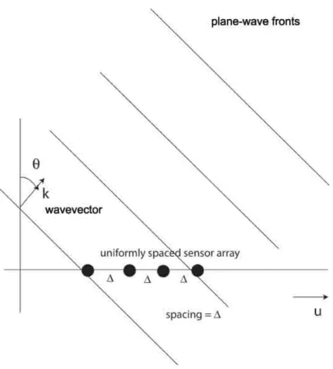
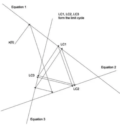
To illustrate how array processing operates, consider Figure 2.1. Imagine a source of acoustic energy sufficiently distant from the line of sensors that the incoming wavefront is essentially planar. As the peaks and troughs of the wavefronts pass over the array of sensors, the measurements at the sensors give the elapsed time between a peak at one sensor and a peak at the next sensor, thereby giving an indication of the angle of arrival.
In practice, of course, there are multiple sources of acoustic energy, so each sensor receives a superposition of all the plane-wave fronts from all directions. because the sensors are spread out in space, what each receives is slightly different from what its neighboring sensors receive, and this slight difference can be exploited to separate the spatially distinct components of the signals. What we seek is the function that describes how much energy came from each direction.
have the problem of estimating a function from finitely many values of its Fourier transform.
2.7
A Word about Prior Information
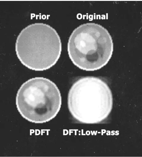
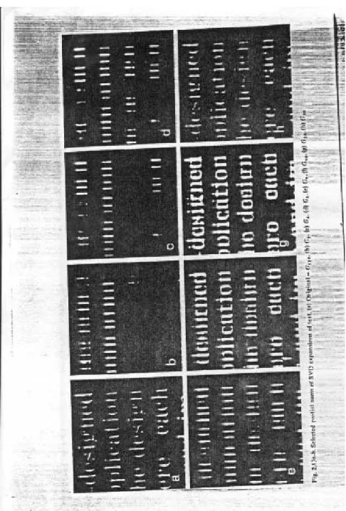
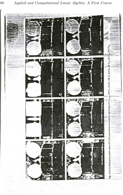
An important point to keep in mind when applying linear-algebraic methods to measured data is that, while the data is usually limited, the information we seek may not be lost. Although processing the data in a reasonable way may suggest otherwise, other processing methods may reveal that the desired information is still available in the data. Figure 2.2 illustrates this point.
The original image on the upper right of Figure 2.2 is a discrete rect-angular array of intensity values simulating a slice of a head. The data was obtained by taking the two-dimensional discrete Fourier transform of the original image, and then discarding, that is, setting to zero, all these spatial frequency values, except for those in a smaller rectangular region around the origin. The problem then is under-determined. A minimum two-norm solution would seem to be a reasonable reconstruction method.
When we weight the skull area with the inverse of the prior image, we allow the reconstruction to place higher values there without having much of an effect on the overall weighted norm. In addition, the reciprocal weighting in the interior makes spreading intensity into that region costly, so the interior remains relatively clear, allowing us to see what is really present there.
Chapter 3
A Little Matrix Theory
3.1 Chapter Summary . . . 21 3.2 Vector Spaces . . . 21 3.3 Matrix Algebra . . . 24 3.3.1 Matrix Operations . . . 24 3.3.2 Matrix Inverses . . . 25 3.3.3 The Sherman-Morrison-Woodbury Identity . . . 26 3.4 Bases and Dimension . . . 27 3.4.1 Linear Independence and Bases . . . 27 3.4.2 Dimension . . . 29 3.4.3 Rank of a Matrix . . . 30 3.5 Representing a Linear Transformation . . . 31 3.6 The Geometry of Euclidean Space . . . 32 3.6.1 Dot Products . . . 32 3.6.2 Cauchy’s Inequality . . . 34 3.7 Vectorization of a Matrix . . . 34 3.8 Solving Systems of Linear Equations . . . 35 3.8.1 Row-Reduction . . . 35 3.8.2 Row Operations as Matrix Multiplications . . . 37 3.8.3 Determinants . . . 37 3.8.4 Sylvester’s Nullity Theorem . . . 38 3.8.5 Homogeneous Systems of Linear Equations . . . 39 3.8.6 Real and Complex Systems of Linear Equations . . . 41 3.9 Under-Determined Systems of Linear Equations . . . 41 3.10 Over-Determined Systems of Linear Equations . . . 43
3.1
Chapter Summary
In this chapter we review the fundamentals of matrix algebra.
3.2
Vector Spaces
Linear algebra is the study ofvector spacesandlinear transformations. It is not simply the study of matrices, although matrix theory takes up most of linear algebra.
It is common in mathematics to consider abstraction, which is simply a means of talking about more than one thing at the same time. A vector spaceV is an abstract algebraic structure defined using axioms. There are many examples of vector spaces, such as the sets of real or complex numbers themselves, the set of all polynomials, the set of row or column vectors of a given dimension, the set of all infinite sequences of real or complex numbers, the set of all matrices of a given size, and so on. The beauty of an abstract approach is that we can talk about all of these, and much more, all at once, without being specific about which example we mean.
A vector space is a set whose members are called vectors, on which there are two algebraic operations, calledscalar multiplication andvector addition. As in any axiomatic approach, these notions are intentionally abstract. A vector is defined to be a member of a vector space, nothing more. Scalars are a bit more concrete, in that scalars are almost always real or complex numbers, although sometimes, but not in this book, they are members of an unspecified finite field. The operations themselves are not explicitly defined, except to say that they behave according to certain axioms, such as associativity and distributivity.
Ifv is a member of a vector space V andαis a scalar, then we denote byαvthe scalar multiplication ofv byα. Ifwis also a member ofV, then we denote byv+wthe vector addition ofvandw. The following properties serve to define a vector space, withu,v, andwdenoting arbitrary members ofV andαandβ arbitrary scalars:
• 1.v+w=w+v;
• 2.u+ (v+w) = (u+v) +w;
• 3. there is a unique “zero vector” , denoted 0, such that, for everyv,
v+ 0 =v;
• 4. for eachv there is a unique vector−v such thatv+ (−v) = 0;
• 5. 1v=v, for allv;
• 6. (αβ)v=α(βv);
• 7.α(v+w) =αv+αw;
Ex. 3.1 Show that, if z+z=z, thenz is the zero vector.
Ex. 3.2 Prove that 0v = 0, for all v ∈ V, and use this to prove that
(−1)v=−v for allv∈V. Hint: use Exercise 3.1.
We then write
w−v=w+ (−v) =w+ (−1)v,
for allv andw.
Ifu1, ..., uN are members ofV andc1, ..., cN are scalars, then the vector
x=c1u1+c2u2+...+cNuN
is called a linear combination of the vectors u1, ..., uN, with coefficients
c1, ..., cN.
If W is a subset of a vector space V, then W is called a subspace of
V if W is also a vector space for the same operations. What this means is simply that when we perform scalar multiplication on a vector in W, or when we add vectors in W, we always get members of W back again. Another way to say this is thatW isclosed to linear combinations.
When we speak of subspaces of V we do not mean to exclude the case ofW =V. Note that V is itself a subspace, but not a proper subspace of
V. Every subspace must contain the zero vector, 0; the smallest subspace ofV is the subspace containing only the zero vector,W ={0}.
Ex. 3.3 Show that, in the vector space V =R2, the subset of all vectors
whose entries sum to zero is a subspace, but the subset of all vectors whose entries sum to one is not a subspace.
Ex. 3.4 Let V be a vector space, andW andY subspaces ofV. Show that the union of W and Y, written W ∪Y, is also a subspace if and only if eitherW ⊆Y orY ⊆W.
We often refer to things like
1 2 0
as vectors, although they are but one example of a certain type of vector. For clarity, in this book we shall call such an object areal row vector of dimension threeor areal row three-vector.
Similarly, we shall call
3i
−1 2 +i
6
acomplex column vector of dimension four
or acomplex column four-vector. For notational convenience, whenever we refer to something like a real three-vector or a complex four-vector, we shall always mean that they are columns, rather than rows. The space of real (column) N-vectors will be denoted RN, while the space of complex (column)N vectors isCN.
notion of the size or dimension of the vector space. A vector space can be finite dimensional or infinite dimensional. The spacesRN andCN have dimensionN; not a big surprise. The vector spaces of all infinite sequences of real or complex numbers are infinite dimensional, as is the vector space of all real or complex polynomials. If we choose to go down the path of finite dimensionality, we very quickly find ourselves talking about matrices. If we go down the path of infinite dimensionality, we quickly begin to discuss convergence of infinite sequences and sums, and find that we need to introduce norms, which takes us into functional analysis and the study of Hilbert and Banach spaces. In this course we shall consider only the finite dimensional vector spaces, which means that we shall be talking mainly about matrices.
3.3
Matrix Algebra
A system Ax= b of linear equations is called a complex system, or a
real systemif the entries of A,x andb are complex, or real, respectively. Note that when we say that the entries of a matrix or a vector are complex, we do not intend to rule out the possibility that they are real, but just to open up the possibility that they are not real.
3.3.1
Matrix Operations
IfAandB are real or complexM byN andN byK matrices, respec-tively, then the productC=ABis defined as theM byK matrix whose entryCmk is given by
Cmk= N
X
n=1
AmnBnk. (3.1)
If x is an N-dimensional column vector, that is, x is an N by 1 matrix, then the productb=Axis theM-dimensional column vector with entries
bm= N
X
n=1
Amnxn. (3.2)
Ex. 3.5 Show that, for each k= 1, ..., K, Colk(C), thekth column of the matrixC=AB, is
It follows from this exercise that, for given matricesAandC, every column of C is a linear combination of the columns of A if and only if there is a third matrixB such thatC=AB.
For any N, we denote by I theN by N identity matrix with entries
In,n = 1 andIm,n = 0, for m, n = 1, ..., N and m 6= n. The size of I is
always to be inferred from the context.
The matrixA† is theconjugate transposeof the matrix A, that is, the
N byM matrix whose entries are
(A†)nm=Amn (3.3)
When the entries ofAare real,A† is just thetransposeofA, writtenAT.
Definition 3.1 A square matrixSissymmetricifST =S andHermitian ifS† =S.
Definition 3.2 A square matrixS isnormalifS†S=SS†. Ex. 3.6 Let C=AB. Show thatC†=B†A†.
Ex. 3.7 LetDbe a diagonal matrix such thatDmm6=Dnnifm6=n. Show that ifBD=DB thenB is a diagonal matrix.
Ex. 3.8 Prove that, ifAB=BAfor everyN byNmatrixA, thenB=cI, for some constantc.
3.3.2
Matrix Inverses
We begin with the definition of invertibility.
Definition 3.3 A square matrixAis said to beinvertible, or to be a non-singularmatrix if there is a matrix B such that
AB=BA=I
whereI is the identity matrix of the appropriate size. There can be at most one such matrixB for a givenA. ThenB =A−1, theinverseof A.
Note that, in this definition, the matricesAand B must commute.
Proposition 3.1 The inverse of a square matrix A is unique; that is, if
The following proposition shows that invertibility follows from an ap-parently weaker condition.
Proposition 3.2 If A is square and there exist matrices B and C such thatAB=I andCA=I, thenB =C=A−1 andAis invertible.
Ex. 3.10 Prove Proposition 3.2.
Later in this chapter, after we have discussed the concept of rank of a matrix, we will improve Proposition 3.2; a square matrix A is invertible if and only if there is a matrix B with AB = I, and, for any (possibly non-square)A, if there are matricesB andC with AB=I and CA=I
(where the twoImay possibly be different in size), thenAmust be square and invertible.
The 2 by 2 matrixS=
a b c d
has an inverse
S−1= 1
ad−bc
d −b
−c a
whenever thedeterminantofS, det(S) =ad−bcis not zero. More generally, associated with every complex square matrix is the complex number called its determinant, which is obtained from the entries of the matrix using formulas that can be found in any text on linear algebra. The significance of the determinant is that the matrix is invertible if and only if its determinant is not zero. This is of more theoretical than practical importance, since no computer can tell when a number is precisely zero. A matrixAthat is not square cannot have an inverse, but does have apseudo-inverse, which can be found using the singular-value decomposition.
Note that, ifAis invertible, thenAx= 0 can happen only whenx= 0. We shall show later, using the notion of the rank of a matrix, that the converse is also true: a square matrix A with the property that Ax = 0 only whenx= 0 must be invertible.
3.3.3
The Sherman-Morrison-Woodbury Identity
In a number of applications, stretching from linear programming to radar tracking, we are faced with the problem of computing the inverse of a slightly modified version of a matrixB, when the inverse ofB itself has already been computed. For example, when we use the simplex algorithm in linear programming, the matrixB consists of some, but not all, of the columns of a larger matrixA. At each step of the simplex algorithm, a new
Bnew is formed fromB=Boldby removing one column ofB and replacing
it with another column taken fromA.
ThenBnew differs fromB in only one column. Therefore
whereuis the column vector that equals the old column minus the new one, andvis the column of the identity matrix corresponding to the column of
Bold being altered. The inverse ofBnew can be obtained fairly easily from
the inverse ofBold using the Sherman-Morrison-Woodbury Identity:
The Sherman-Morrison-Woodbury Identity:IfvTB−1u6= 1, then
(B−uvT)−1=B−1+α−1(B−1u)(vTB−1), (3.5) where
α= 1−vTB−1u.
Ex. 3.11 Let B be invertible andvTB−1u= 1. Show that B−uvT is not invertible. Show that Equation (3.5) holds, ifvTB−1u6= 1.
3.4
Bases and Dimension
The related notions of a basis and of linear independence are funda-mental in linear algebra.
3.4.1
Linear Independence and Bases
As we shall see shortly, the dimension of a finite-dimensional vector space will be defined as the number of members of any basis. Obviously, we first need to see what a basis is, and then to convince ourselves that if a vector spaceV has a basis withN members, then every basis forV has
N members.
Definition 3.4 Thespanof a collection of vectors{u1, ..., uN}inV is the set of all vectors x that can be written as linear combinations of the un; that is, for which there are scalars c1, ..., cN, such that
x=c1u1+...+cNuN. (3.6) Definition 3.5 A collection of vectors{w1, ..., wN} inV is called a
span-ning setfor a subspace W if the set W is their span.
Definition 3.6 A subspaceW of a vector spaceV is called finite dimen-sionalif it is the span of a finite set of vectors fromV. The whole spaceV