Micro-Unit 3b-Perfect Competition.pdf

Perfect Competition in the

Short Run & the Long Run

A FIRM’S PROFIT-MAXIMIZING CHOICES



Price Taker

– A price taker is a firm that cannot influence the price of the good or service that it produces. – The firm in perfect competition is a price taker. Section

A FIRM’S PROFIT-MAXIMIZING CHOICES



Revenue Concepts

– In perfect competition, market demand and market supply determine price.

– A firm’s total revenue equals the market price multiplied by the quantity sold.

– A firm’s marginal revenue is the change in total revenue that results from a one-unit increase in the quantity sold.

A FIRM’S PROFIT-MAXIMIZING CHOICES

A FIRM’S PROFIT-MAXIMIZING CHOICES

A FIRM’S PROFIT-MAXIMIZING CHOICES

A FIRM’S PROFIT-MAXIMIZING CHOICES

Dave’s total revenue curve is TR.

A FIRM’S PROFIT-MAXIMIZING CHOICES



Profit-Maximizing Output

– As output increases, total revenue increases. – But total cost also increases.

– Because of decreasing marginal returns, total cost eventually increases faster than total revenue.

– There is one output level that maximizes

A FIRM’S PROFIT-MAXIMIZING CHOICES

– One way to find the profit-maximizing output is to use a firm’s total revenue and total cost curves. – Profit is maximized at the output level at which

total revenue exceeds total cost by the largest amount.

A FIRM’S PROFIT-MAXIMIZING CHOICES

as the quantity

increases —shown by the TR curve.

Total cost increases as the quantity

increases—shown by the TC curve.

As the quantity

increases, economic profit (TR – TC)

A FIRM’S PROFIT-MAXIMIZING CHOICES

At low output levels, the firm incurs an economic loss.

When total revenue exceeds total cost, the firm earns an economic profit.

Profit is maximized when the gap

between total

revenue and total

A FIRM’S PROFIT-MAXIMIZING CHOICES



Marginal Analysis and the Supply Decision

MR, with marginal cost, MC.

– As output increases, marginal revenue remains constant but marginal cost increases.

– If marginal revenue exceeds marginal cost (if MR > MC), the extra revenue from selling one more unit exceeds the extra cost incurred to produce it.

A FIRM’S PROFIT-MAXIMIZING CHOICES

– If marginal revenue is less than marginal cost (if MR < MC), the extra revenue from selling one more unit is less than the extra cost incurred to produce it.

– Economic profit increases if output decreases. – If marginal revenue equals marginal cost (if MR =

MC), the extra revenue from selling one more unit is equal to the extra cost incurred to produce it. – Economic profit decreases if output increases or

Figure 15.3 shows the profit-maximizing output.

Marginal revenue is a constant $8 per can.

Marginal cost decreases at low outputs but then increases.

1. Profit is maximized when marginal revenue equals marginal cost at 10 cans a day.

2. If output increases from 9 to 10 cans a day, arginal cost ($7) is below marginal revenue ($8), so profit increases.

3. If output increases from 10 to 11 cans a day,

marginal cost ($9) exceeds marginal revenue ($8), so profit decreases.

The Perfectly Competitive Firm

1. How is the price established at which the firm sells?

The Perfectly Competitive Firm

3. Why do we say a perfect competitor is a price taker?

The Perfectly Competitive Firm

2. How much control does the firm have over this price?

The Perfectly Competitive Firm

4. Why does a perfect competitor maximize profits where Price = MC?

The Perfectly Competitive Firm

5. Is this perfect competitor making a profit? Why or why not?

A FIRM’S PROFIT-MAXIMIZING CHOICES



Temporary Shutdown Decisions

– If a firm is incurring an economic loss that it

believes is temporary, it will remain in the market, and it might produce some output or temporarily shut down.

Section

A FIRM’S PROFIT-MAXIMIZING CHOICES

– If the firm shuts down temporarily, it incurs an economic loss equal to total fixed cost.

– If the firm produces some output, it incurs an economic loss equal to total fixed cost plus total variable cost minus total revenue.

– If total revenue exceeds total variable cost, the

A FIRM’S PROFIT-MAXIMIZING CHOICES

– If total revenue were less than total variable cost, the firm’s economic loss would exceed total fixed cost. So the firm would shut down temporarily. – Total fixed cost is the largest economic loss that

the firm will incur.

– The firm’s economic loss equals total fixed cost when price equals average variable cost.

A FIRM’S PROFIT-MAXIMIZING CHOICES

– The firm’s shutdown point is the output and price

at which price equals minimum average variable cost.

A FIRM’S PROFIT-MAXIMIZING CHOICES

Marginal revenue curve is

MR.

A FIRM’S PROFIT-MAXIMIZING CHOICES

1. With a market price (and MR) of $3 a can, the firm

A FIRM’S PROFIT-MAXIMIZING CHOICES

A FIRM’S PROFIT-MAXIMIZING CHOICES



The Firm’s Short-Run Supply Curve

– A perfectly competitive firm’s short-run supply curve shows how the firm’s profit-maximizing output varies as the price varies, other things remaining the same.

– Figure 15.5 on the next slide illustrates a firm’s

FIRM’S … CHOICES

curve is AVC, and its marginal revenue curve is MR₀.

Point T is one point on the firm’s supply curve.

With a market price (and MR₀) of $3 a can, the firm

FIRM’S … CHOICES

If the market price rises to $8 a can, the marginal revenue curve shifts upward to MR₁.

Profit-maximizing output

increases to 10 cans per day.

FIRM’S … CHOICES

If the price rises to $12 a can, the marginal revenue curve shifts upward to MR₂.

Profit-maximizing output

increases to 11 cans per day.

The new black dot in part (b) is another point of the firm’s

supply curve.

The blue curve is the firm’s supply curve.

At prices below $3 a can, the firm shuts down and output is zero.

At prices above $3 a can, the firm produces along its

MC curve.

The supply curve is the

same as the MC curve at

prices above the minimum point of AVC.

OUTPUT, PRICE, PROFIT IN THE

SHORT RUN



_{Market Supply in the Short Run}

– The market supply curve in the short run shows the quantity supplied at each price by a fixed number of firms.

– The quantity supplied at a given price is the sum of the quantities supplied by all firms at that price.

Figure 15.6 on the next slide shows the market

At the shutdown price of $3, each firm produces either 0 or 7 cans a day.

OUTPUT, PRICE, PROFIT IN THE SHORT RUN

At prices above the shutdown price, firms produce

along their MC curve.

OUTPUT, PRICE, PROFIT IN THE SHORT RUN

The market supply curve:

Below the shutdown price, it runs along the y-axis. At the shutdown price, it is perfectly elastic.

In part (a), with market supply curve, S, and market

demand curve, D₁, the market price is $5 a can.

OUTPUT, PRICE, PROFIT IN THE

SHORT RUN



_{Short-Run Equilibrium in Normal Times}

– Market demand and market supply determine the market price and quantity bought and sold.

In part (a), with market supply curve, S, and market

demand curve, D₁, the market price is $5 a can.

In part (b), marginal revenue is $5 a can.

Dave produces 9 cans a day, where marginal cost equals marginal revenue.

At this quantity, price equals average total cost, so Dave makes zero economic profit.

OUTPUT, PRICE, PROFIT IN THE

SHORT RUN



Short-Run Equilibrium in Good Times

– In the short-run equilibrium that we’ve just examined, Dave made zero economic profit.

– Although such an outcome is normal, economic profit can be positive or negative in the short run. – Figure 15.8 on the next slide illustrates short-run

In part (a), with market demand curve D₂ and

market supply curve S, the market price is $8 a

can.

In part (b), Dave’s marginal revenue is $8 a can. Dave produces 10 cans a day, where marginal cost equals marginal revenue.

At this quantity, price ($8 a can) exceeds average total cost ($5.10 a can).

Dave makes an economic profit shown by the blue rectangle.

OUTPUT, PRICE, PROFIT IN THE

SHORT RUN



Short-Run Equilibrium in Bad Times

– In the short-run equilibrium that we’ve just

examined, Dave is enjoying an economic profit. – But such an outcome is not inevitable.

In part (a), with the market supply curve, S, and the

market market demand curve, D₃, the market price

is $3 a can.

In part (b), Dave’s marginal revenue is $3 a can.

Dave produces 7 cans a day, where marginal cost equals marginal revenue and not less than average variable cost.

At this quantity, price ($3 a can) is less than average total cost ($5.14 a can).

Dave incurs an economic loss shown by the red rectangle.

Profit, Loss and Shutdown for a

Perfectly Competitive Firm

1. At what output will the firm

operate at price P₄, Q₄?

Profit, Loss and Shutdown for a

Perfectly Competitive Firm

2. At price P₃, will the firm make a profit, break

even, or have an economic loss?

Break even

What does it mean to break even?

Profit, Loss and Shutdown for a

Perfectly Competitive Firm

3. At price P₂, will the firm make a profit, break even, or have an economic loss?

Economic loss

Will it continue to produce? Why or why not?

Profit, Loss and Shutdown for a

Perfectly Competitive Firm

4. At price P₁, will the firm make a profit, break

even, or have an economic loss?

Profit, Loss and Shutdown for a

Perfectly Competitive Firm

Will it continue to produce? Why or why not?

Indifferent. If firm produces, revenue covers variable

The Perfectly

Competitive

Firm in Long-Run

Equilibrium

 The market price is determined by supply and



Once the price

is established,

every firm

must sell at

that price or

not sell at all.

There is no

reason for a

firm to lower

its price since it

can already sell

as much as it

wants.



If firms are

making

economic

profits, more

firms will enter

the industry –

an event that

reduces and

makes profits

disappear.



If firms have

economic

losses, firms

will exit the

market – an

event that will

cause the price

to rise.

 A perfectly

competitive firm is long-run

equilibrium is good for society because there is productive and allocative

efficiency when the firm is at the lowest point on its average total cost curve.

OUTPUT, PRICE, PROFIT IN THE

LONG RUN

– Neither good times nor bad times last forever in perfect competition.

– In the long run, a firm in perfect competition makes zero profit.

– Figure 15.10 on the next slide illustrates equilibrium in the long run.

Section

Part (a) illustrates the firm in long-run equilibrium. The market price is $5 a can and Dave produces 9 cans a day.

In part (a), minimum ATC is $5 a can.

In the long run, Dave produces at minimum ATC.

If supply decreases, the price rises above $5 a can and Dave will make a positive economic profit.

Entry increases supply to S and the price falls to $5 a

can.

If supply increases, the price falls below $5 a can and Dave incurs an economic loss.

Exit decreases supply to S and the price rises to $5 a

can.

In the long-run, the price is pulled to $5 a can and Dave makes zero economic profit.

OUTPUT, PRICE, PROFIT IN THE

LONG RUN



_{Entry and Exit}

– In the long run, firms respond to economic profit and economic loss by either entering or exiting a market.

– New firms enter a market in which the existing firms are making positive economic profits.

– Existing firms exit the market in which firms are incurring economic losses.

OUTPUT, PRICE, PROFIT IN THE

LONG RUN

– The immediate effect of the decision to enter or exit is to shift the market supply curve.

– If more firms enter a market, supply increases and the market supply curve shifts rightward.

OUTPUT, PRICE, PROFIT IN THE

LONG RUN

– The Effects of Entry

OUTPUT, PRICE, PROFIT IN THE LONG RUN

Figure 15.11 shows the effects of entry.

Starting in long-run equilibrium,

1. If demand increases

from D₀ to D₁, the price rises from $5 to $8 a can.

OUTPUT, PRICE, PROFIT IN THE LONG RUN

2. As firms enter the market, the supply curve shifts

rightward, from S₀ to S₁.

Economic profit brings entry.

The equilibrium price

falls from $8 to $5 a can, and the quantity

OUTPUT, PRICE, PROFIT IN THE

LONG RUN



_{The Effects of Exit}

OUTPUT, PRICE, PROFIT IN THE LONG RUN

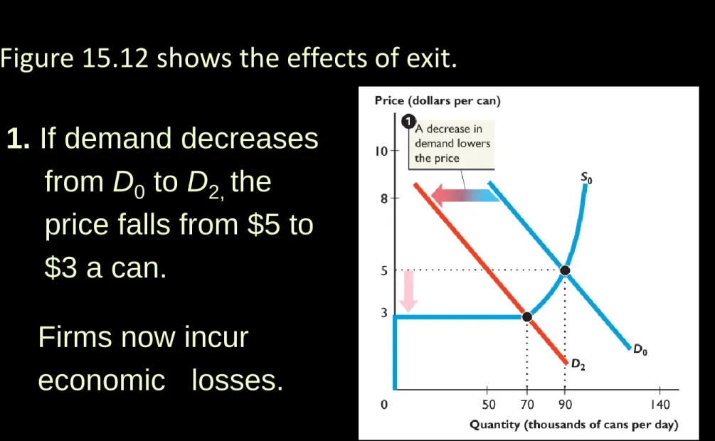
Figure 15.12 shows the effects of exit.

Starting in long-run equilibrium, 1. If demand decreases

from D₀ to D_2, the

price falls from $5 to $3 a can.

OUTPUT, PRICE, PROFIT IN THE LONG RUN

2. As firms exit the market, the supply curve shifts leftward, from S₀ to S₂.

Economic loss brings exit.

The equilibrium price rises from $3 to $5 a can, and the quantity produced

OUTPUT, PRICE, PROFIT IN THE LONG RUN



_{Change in Demand}

– The difference between the initial long-run

equilibrium and the final long-run equilibrium is the number of firms in the market.

– An increase in demand increases the number of firms. Each firm produces the same output in the new long-run equilibrium as initially and makes zero economic profit.

– In the process of moving from the initial

OUTPUT, PRICE, PROFIT IN THE

LONG RUN

– A decrease in demand triggers a similar response, except in the opposite direction.

– The decrease in demand brings a lower price, economic loss, and some firms exit.

OUTPUT, PRICE, PROFIT IN THE

LONG RUN



Technological Change

– New technology allows firms to produce at a lower cost. As a result, as firms adopt a new technology, their cost curves shift downward. – Market supply increases, and the market supply

curve shifts rightward.

OUTPUT, PRICE, PROFIT IN THE

LONG RUN

Two forces are at work in a market undergoing technological change.

1. Firms that adopt the new technology make an economic profit.

– So new-technology firms have an incentive to enter.

2. Firms that stick with the old technology incur economic losses.

OUTPUT, PRICE, PROFIT IN THE LONG RUN



Is Perfect Competition Efficient?

– Resources are used efficiently when it is not

possible to get more of one good without giving up something that is valued more highly.

– To achieve this outcome, marginal benefit must equal marginal cost. That is what perfect

competition achieves.

– The market supply curve is the marginal cost curve. It is the sum of the firms’ marginal cost

OUTPUT, PRICE, PROFIT IN THE

LONG RUN

– The market supply curve is the marginal cost curve.

– The market demand curve is the marginal benefit curve.

– Because the market supply and market demand curves intersect at the equilibrium price, that price equals both marginal cost and marginal benefit.

OUTPUT, PRICE, PROFIT IN THE LONG RUN

1. Market equilibrium

occurs at a price of $5 a can and a quantity of 90,000 cans a day.

2. Supply curve is also the marginal cost

curve.

3. Demand curve is also

OUTPUT, PRICE, PROFIT IN THE LONG RUN

Because marginal benefit equals marginal cost

4. Efficient quantity is produced.

OUTPUT, PRICE, PROFIT IN THE

LONG RUN



Is Perfect Competition Fair?

– Perfect competition places no restrictions on

anyone’s actions—everyone is free to try to make an economic profit.

– The process of competition eliminates economic profit and brings maximum attainable benefit to consumers.

– Fairness as equality of opportunity and fairness as equality of outcomes are achieved in long-run

OUTPUT, PRICE, PROFIT IN THE

LONG RUN

– But in the short run, economic profit and economic loss can arise.

How an Increase in Demand Changes Long-Run

Equilibrium for the Firm and Industry

How a Decrease in Demand Changes Long-Run

Equilibrium for the Firm and Industry

Why Did GM Fail?

In 2008, the average price at which old GM could sell a vehicle was $18,000.

To maximize profit (minimize loss), GM sold 8 million

vehicles.

Average total cost of 8 million vehicles was $22,000, so the economic loss was $4,000 per vehicle.

Why Did GM Fail?

The firm’s “restructuring” has plans for cost savings and

investment in new green technology vehicles.

Why Did GM Fail?

Cutting fixed cost is the only way that the new GM can have a major impact on its profitability.

The minimum that the new GM must do is cut fixed cost to shift its ATC curve down from ATC_O to ATC_N.

GM can then maximize profit at the same quantity, 8