The Haskell School of Music
— From Signals to Symphonies —
Paul Hudak
Yale University
Department of Computer Science
The Haskell School of Music — From Signals to Symphonies —
Paul Hudak Yale University
Department of Computer Science New Haven, CT, USA Version 2.4 (February 22, 2012)
Copyright cPaul Hudak January 2011
All rights reserved. No part of this publication may be reproduced or distributed in any form or by any means, or stored in a data base or retrieval system, without the prior written permission of the author.
Contents
Preface xiv
1 Overview of Computer Music, Euterpea, and Haskell 1
1.1 The Note vs. Signal Dichotomy . . . 2
1.2 Basic Principles of Programming . . . 3
1.3 Computation by Calculation. . . 4
1.4 Expressions and Values . . . 8
1.5 Types . . . 10
1.6 Function Types and Type Signatures . . . 11
1.7 Abstraction, Abstraction, Abstraction . . . 13
1.7.1 Naming . . . 13
1.7.2 Functional Abstraction. . . 16
1.7.3 Data Abstraction . . . 19
1.8 Haskell Equality vs. Euterpean Equality . . . 22
1.9 Code Reuse and Modularity . . . 23
1.10 [Advanced] Programming with Numbers . . . 24
2 Simple Music 28 2.1 Preliminaries . . . 28
2.2 Notes, Music, and Polymorphism . . . 30
2.3 Convenient Auxiliary Functions . . . 33
2.3.1 A Simple Example . . . 35
2.4 Absolute Pitches . . . 39
3 Polymorphic & Higher-Order Functions 43
3.1 Polymorphic Types . . . 44
3.2 Abstraction Over Recursive Definitions. . . 45
3.2.1 Map is Polymorphic . . . 47
3.2.2 Using map . . . 48
3.3 Append . . . 49
3.3.1 [Advanced] The Efficiency and Fixity of Append . . . 50
3.4 Fold . . . 51
3.4.1 Haskell’s Folds . . . 53
3.4.2 [Advanced] Why Two Folds? . . . 54
3.4.3 Fold for Non-empty Lists . . . 55
3.5 [Advanced] A Final Example: Reverse . . . 56
3.6 Currying. . . 57
3.6.1 Currying Simplification . . . 59
3.6.2 [Advanced] Simplification of reverse . . . 60
3.7 Errors . . . 61
4 A Musical Interlude 64 4.1 Modules . . . 64
4.2 Transcribing an Existing Score . . . 65
4.2.1 Auxiliary Functions . . . 67
4.2.2 Bass Line . . . 68
4.2.3 Main Voice . . . 69
4.2.4 Putting It All Together . . . 69
4.3 Simple Algorithmic Composition . . . 71
5 Syntactic Magic 72 5.1 Sections . . . 72
5.2 Anonymous Functions . . . 74
5.3 List Comprehensions . . . 75
5.3.1 Arithmetic Sequences . . . 77
5.5 Higher-Order Thinking. . . 79
5.6 Infix Function Application . . . 80
6 More Music 82 6.1 Delay and Repeat. . . 82
6.2 Inversion and Retrograde . . . 83
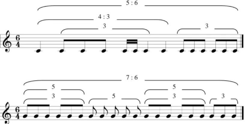
6.3 Polyrhythms . . . 84
6.4 Symbolic Meter Changes . . . 86
6.5 Computing Duration . . . 86
6.6 Super-retrograde . . . 87
6.7 Truncating Parallel Composition . . . 88
6.8 Trills . . . 89
6.9 Grace Notes . . . 90
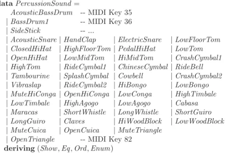
6.10 Percussion . . . 91
6.11 A Map for Music . . . 93
6.12 A Fold for Music . . . 94
6.13 Crazy Recursion . . . 95
7 Qualified Types and Type Classes 98 7.1 Motivation . . . 98
7.2 Equality . . . 100
7.3 Defining Your Own Type Classes . . . 102
7.4 Inheritance . . . 106
7.5 Haskell’s Standard Type Classes . . . 107
7.5.1 The Num Class . . . 108
7.5.2 The Show Class . . . 111
7.6 Derived Instances . . . 112
7.7 Reasoning With Type Classes . . . 115
8 Interpretation and Performance 118 8.1 Abstract Performance . . . 118
8.2.1 Example of Player Construction . . . 126
8.2.2 Deriving New Players From Old Ones . . . 128
8.2.3 A Fancy Player . . . 129
8.3 Putting it all Together . . . 129
9 Self-Similar Music 133 9.1 Self-Similar Melody. . . 133
9.1.1 Sample Compositions . . . 136
9.2 Self-Similar Harmony. . . 137
9.3 Other Self-Similar Structures . . . 138
10 Proof by Induction 141 10.1 Induction and Recursion . . . 141
10.2 Examples of List Induction . . . 142
10.3 Proving Function Equivalences . . . 144
10.3.1 [Advanced] Reverse. . . 145
10.4 Useful Properties on Lists . . . 147
10.4.1 [Advanced] Function Strictness . . . 150
10.5 Induction on the Music Data Type . . . 151
10.5.1 The Need for Musical Equivalence . . . 156
10.6 [Advanced] Induction on Other Data Types . . . 156
10.6.1 A More Efficient Exponentiation Function . . . 158
11 An Algebra of Music 163 11.1 Musical Equivalance . . . 163
11.2 Some Simple Axioms . . . 165
11.3 The Axiom Set . . . 168
11.4 Soundness and Completeness . . . 169
12 Musical L-Systems 170 12.1 Generative Grammars . . . 170
12.2 A Simple Implementation . . . 171
12.4 An L-System Grammar for Music . . . 175
12.5 Examples . . . 176
13 Random Numbers ... and Markov Chains 179 13.1 Random Numbers . . . 179
13.2 Probability Distributions. . . 182
13.2.1 Random Melodies and Random Walks . . . 186
13.3 Markov Chains . . . 188
13.3.1 Training Data. . . 189
14 From Performance to Midi 192 14.1 An Introduction to Midi . . . 192
14.1.1 General Midi . . . 193
14.1.2 Channels and Patch Maps . . . 194
14.1.3 Standard Midi Files . . . 196
14.2 Converting a Performance into Midi . . . 198
14.3 Putting It All Together . . . 201
15 Basic Input/Output 202 15.1 IO in Haskell . . . 202
15.2 doSyntax . . . 204
15.3 Actions are Just Values . . . 205
15.4 Reading and Writing Midi Files . . . 207
16 Musical User Interface 208 16.1 Signals . . . 209
16.1.1 Numeric Signals . . . 210
16.1.2 Time. . . 211
16.1.3 Musical Signals . . . 212
16.1.4 Useful Signal Operators . . . 213
16.1.5 Stateful Signals . . . 213
16.2 Events and Reactivity . . . 214
16.2.2 Turning Signals into Events . . . 215
16.2.3 Signal Samplers. . . 216
16.2.4 Switches and Reactivity . . . 216
16.3 The UI Level . . . 217
16.3.1 Input Widgets . . . 217
16.3.2 UI Transformers . . . 220
16.3.3 MIDI Input and Output . . . 221
16.3.4 Midi Device IDs . . . 222
16.3.5 Timer Widgets . . . 224
16.4 Putting It All Together . . . 225
16.5 Musical Examples . . . 225
16.5.1 Chord Builder . . . 225
16.5.2 Bifurcate Me, Baby! . . . 227
16.5.3 MIDI Echo Effect. . . 229
17 Sound and Signals 231 17.1 The Nature of Sound . . . 231
17.1.1 Frequency and Period . . . 234
17.1.2 Amplitude and Loudness . . . 235
17.1.3 Frequency Spectrum . . . 239
17.2 Digital Audio . . . 241
17.2.1 From Continuous to Discrete . . . 243
17.2.2 Fixed-Waveform Table-Lookup Synthesis . . . 245
17.2.3 Aliasing . . . 246
17.2.4 Quantization Error . . . 249
17.2.5 Dynamic Range. . . 251
18 Euterpea’s Signal Functions 253 18.1 Signals and Signal Functions . . . 254
18.1.1 The Type of a Signal Function . . . 256
18.1.2 Four Useful Functions . . . 258
18.2 Generating Sound . . . 264
18.3 Instruments . . . 266
18.3.1 Turning a Signal Function into an Instruement . . . . 266
18.3.2 Envelopes . . . 269
19 Spectrum Analysis 273 19.1 Fourier’s Theorem . . . 273
19.1.1 The Fourier Transform . . . 275
19.1.2 Examples . . . 276
19.2 The Discrete Fourier Transform . . . 277
19.2.1 Interpreting the Frequency Spectrum. . . 280
19.2.2 Amplitude and Power of Spectrum . . . 282
19.2.3 A Haskell Implementation of the DFT . . . 284
19.3 The Fast Fourier Transform . . . 290
19.4 Further Pragmatics . . . 291
19.5 References . . . 292
20 Additive Synthesis and Amplitude Modulation 294 20.1 Preliminaries . . . 294
20.2 A Bell Sound . . . 295
20.3 Amplitude Modulation . . . 298
20.3.1 AM Sound Synthesis . . . 299
20.4 What do Tremolo and AM Radio Have in Common? . . . 300
A The PreludeList Module 302 A.1 The PreludeList Module . . . 303
A.2 Simple List Selector Functions . . . 303
A.3 Index-Based Selector Functions . . . 304
A.4 Predicate-Based Selector Functions . . . 306
A.5 Fold-like Functions . . . 306
A.6 List Generators . . . 308
A.8 Boolean List Functions . . . 309
A.9 List Membership Functions . . . 310
A.10 Arithmetic on Lists . . . 310
A.11 List Combining Functions . . . 311
B Haskell’s Standard Type Classes 313 B.1 The Ordered Class . . . 313
B.2 The Enumeration Class . . . 314
B.3 The Bounded Class . . . 315
B.4 The Show Class . . . 316
B.5 The Read Class . . . 319
B.6 The Index Class . . . 322
B.7 The Numeric Classes . . . 323
C Built-in Types Are Not Special 325
List of Figures
1.1 Polyphonic vs. Contrapuntal Interpretation . . . 23
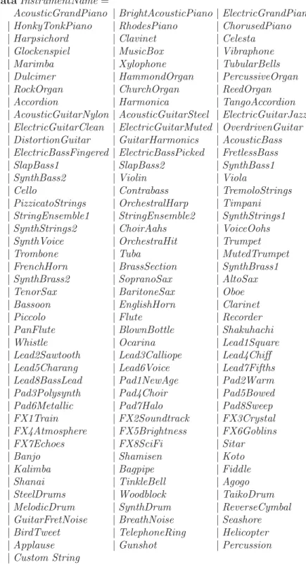
2.1 General MIDI Instrument Names . . . 34
2.2 Convenient Note Names . . . 36
2.3 Convenient Duration and Rest Names . . . 37
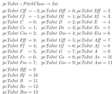
2.4 Converting Pitch Classes to Integers . . . 41
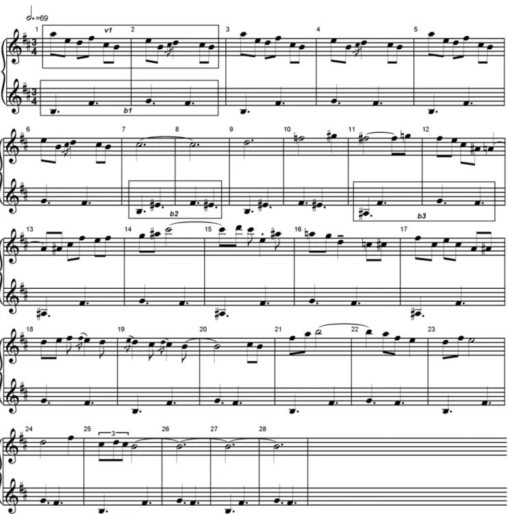
4.1 Excerpt from Chick Corea’s Child Song No. 6 . . . 66
4.2 Bars 7-28 . . . 70
5.1 Gluing Two Functions Together . . . 78
6.1 Nested Polyrhythms (top: pr1; bottom: pr2) . . . 85
6.2 Trills inStars and Stripes Forever . . . 90
6.3 General MIDI Percussion Names . . . 92
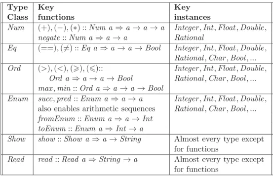
7.1 Common Type Classes and Their Instances . . . 108
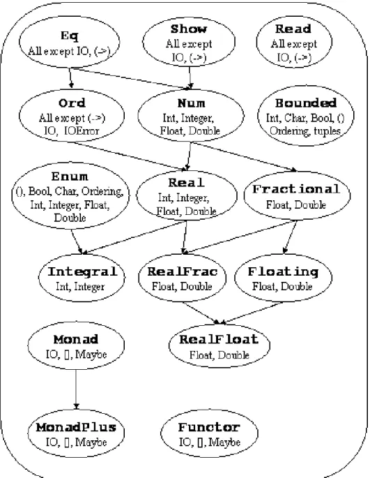
7.2 Numeric Class Hierarchy . . . 110
7.3 Standard Numeric Types . . . 111
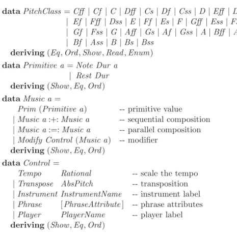
7.4 Euterpea’s Data Types with Deriving Clauses . . . 114
8.1 An abstractperform function . . . 121
8.2 A more efficient perform function . . . 123
8.3 Phrase Attributes. . . 125
8.4 Definition of default playerdefPlayer. . . 127
8.5 Definition of PlayerfancyPlayer. . . 132
9.1 An Example of Self-Similar Music . . . 134
10.1 Proof that f x n∗f x n =f (x∗x)n. . . . 161
13.1 Various Probability Density Functions . . . 183
14.1 Partial Definition of the Midi Data Type . . . 197
16.1 Several Simple MUIs . . . 219
16.2 A Chord Builder MUI . . . 226
17.1 A Sine Wave . . . 232
17.2 RMS Amplitude for Different Signals . . . 236
17.3 Fletcher-Munson Equal Loudness Contour . . . 238
17.4 Spectral Plots of Different Signals. . . 240
17.5 Time-Varying Spectral Plots. . . 242
17.6 Choice of Sampling Rate . . . 244
17.7 Aliasing 1 . . . 247
17.8 Aliasing 2 . . . 248
17.9 A Properly Sampled Signal . . . 250
17.10Block Diagram of Typical Digital Audio System. . . 250
18.1 Eutperea’s Oscillators . . . 260
18.2 Table Generating Functions . . . 262
18.3 A Simple Melody . . . 269
18.4 A Complete Example of a Signal-Function Based Instrument 270 18.5 Envelopes . . . 271
19.1 Examples of Fourier Transforms. . . 278
19.2 Generating a Square Wave from Odd Harmonics . . . 279
19.3 Complex and Polar Coordinates. . . 283
19.4 Helper Code for Pretty-Printing DFT Results . . . 286
20.1 Working With Lists of Signal Sources . . . 295
20.2 A Bell Instrument . . . 296
20.3 A More Sophisticated Bell Instrument . . . 297
10.1 Some Useful Properties of map and fold. . . . 148
10.2 Useful Properties of Other Functions Over Lists. . . 149
13.1 Second-Order Markov Chain . . . 189
14.1 General Midi Instrument Families. . . 194
16.1 Signal Samplers . . . 216
16.2 MUI Input Widgets . . . 217
16.3 MUI Layout Widget Transformers . . . 220
Preface
In the year 2000 I wrote a book called The Haskell School of Expression – Learning Functional Programming through Multimedia [Hud00]. In that book I used graphics, animation, music, and robotics as a way to motivate learning how to program, and specifically how to learnfunctional program-ming using Haskell, a purely functional programming language. Haskell [P+03] is quite a bit different from conventional imperative or object-oriented languages such as C, C++, Java, C#, and so on. It takes a different mind-set to program in such a language, and appeals to the mathematically inclined and to those who seek purity and elegance in their programs. Although Haskell was designed over twenty years ago, it has only recently begun to catch on in a significant way, not just because of its purity and elegance, but because with it you can solve real-world problems quickly and efficiently, and with great economy of code.
I have also had a long, informal, yet passionate interest in music, being an amateur jazz pianist and having played in several bands over the years. About fifteen years ago, in an effort to combine work with play, I and my students wrote a Haskell library called Haskore for expressing high-level computer music concepts in a purely functional way [HMGW96, Hud96, Hud03]. Indeed, three of the chapters in The Haskell School of Expression summarize the basic ideas of this work. Soon after that, with the help of another student, Matt Zamec, I designed a Haskell library called HasSound that was, essentially, a Haskell interface to csound [Ver86] for doing sound synthesis and instrument design.
Thus, when I recently became responsible for the Music Track in the new Computing and the Arts major at Yale, and became responsible for teaching not one, but two computer music courses in the new curriculum, it was natural to base the course material on Haskell. This current book is a rewrite ofThe Haskell School of Expression with a focus on computer music, based on, and greatly improving upon, the ideas in Haskore and HasSound.
The new Haskell library that incorporates all of this is calledEuterpea. Haskell was named after the logician Haskell B. Curry who, along with Alonzo Church, helped establish the theoretical foundations of functional programming in the 1940’s, when digital computers were mostly just a gleam in researchers’ eyes. A curious historical fact is that Haskell Curry’s father, Samuel Silas Curry, helped found and direct a school in Boston called the School of Expression. (This school eventually evolved into what is nowCurry College.) Since pure functional programming is centered around the notion of anexpression, I thought that The Haskell School of Expressionwould be a good title for my first book. And it was thus quite natural to chooseThe Haskell School of Music for my second!
How To Read This Book
As mentioned earlier, there is a certain mind-set, a certain viewpoint of the world, and a certain approach to problem solving that collectively work best when programming in Haskell (this is true for any programming paradigm). If you teach only Haskell language details to a C programmer, he or she is likely to write ugly, incomprehensible functional programs. But if you teach how to think differently, how to see problems in a different light, functional solutions will come easily, and elegant Haskell programs will result. As Samuel Silas Curry once said:
All expression comes from within outward, from the center to the surface, from a hidden source to outward manifestation. The study of expression as a natural process brings you into contact with cause and makes you feel the source of reality.
What is especially beautiful about this quote is that music is also a form of expression, although Curry was more likely talking about writing and speech. In addition, as has been noted by many, music has many ties to mathematics. So for me, combining the elegant mathematical nature of Haskell with that of music is as natural as singing a nursery tune.
that are elegant, concise, yet powerful. We will consistently attempt to let the music express itself as naturally as possible, without encoding it in terms of irrelevant language details.
Of course, my ultimate goal is not just to teach computer music concepts. Along the way you will also learn Haskell. There is no limit to what one might wish to do with computer music, and therefore the better you are at programming, the more success you will have. This is why I think that many languages designed specifically for computer music—although fun to work with, easy to use, and cute in concept—face the danger of being too limited in expressiveness.
You do not need to know much, if any, music theory to read this book, and you do not need to play an instrument. Of course, the more you know about music, the more you will be able to apply the concepts learned in this text in musically creative ways.
My general approach to introducing computer music concepts is to first provide an intuitive explanation, then a mathematically rigorous definition, and finally fully executable Haskell code. In the process I introduce Haskell features as they are needed, rather than all at once. I believe that this interleaving of concepts and applications makes the material easier to digest. Another characteristic of my approach is that I do not hide any details—I want Euterpea to be as transparent as possible! There are no magical built-in operations, no special computer music commands or values. This works out well for several reasons. First, there is in fact nothing ugly or difficult to hide—so why hide anything at all? Second, by reading the code, you will better and more quickly understand Haskell. Finally, by stepping through the design process with me, you may decide that you prefer a different approach—there is, after all, no One True Way to express computer music ideas. I expect that this process will position you well to write rich, creative musical applications on your own.
style changes for the better.
I also ask the experienced programmer to be patient while in the earlier chapters I explain things like “syntax,” “operator precedence,” etc., since it is my goal that this text should be readable by someone having only modest prior programming experience. With patience the more advanced ideas will appear soon enough.
If you are a novice programmer, I suggest taking your time with the book; work through the exercises, and don’t rush things. If, however, you don’t fully grasp an idea, feel free to move on, but try to re-read difficult material at a later time when you have seen more examples of the concepts in action. For the most part this is a “show by example” textbook, and you should try to execute as many of the programs in this text as you can, as well as every program that you write. Learn-by-doing is the corollary to show-by-example.
Finally, I note that some section titles are prefaced with the parenthetical phrase, “[Advanced]”. These sections may be skipped upon first reading, especially if the focus is on learning computer music concepts, as opposed to programming concepts.
Haskell Implementations
There are several good implementations of Haskell, all available free on the Internet through the Haskell users’ website at http://haskell.org. One that I especially recommend isGHC, an easy-to-use and easy-to-install Haskell compiler and interpreter (see http://haskell.org/ghc). GHC runs on a variety of platforms, including PC’s (Windows 7, XP, and Vista), various flavors of Unix (Linux, FreeBSD, etc.), and Mac OS X. The preferred way to install GHC is through theHaskell Platform
(http://hackage.haskell.org/platform/). Any text editor can be used to create source files, but I prefer to use emacs (see
Acknowledgements
I wish to thank my funding agencies—the National Science Foundation, the Defense Advanced Research Projects Agency, and Microsoft Research—for their generous support of research that contributed to the foundations of Euterpea. Yale University has provided me a stimulating and flexible envi-ronment to pursue my dreams for almost thirty years, and I am especially thankful for its recent support of the Computing and the Arts initiative.
Tom Makucevich, a talented computer music practitioner and composer in New Haven, was the original motivator, and first user, of Haskore, which preceded Euterpea. Watching him toil endlessly with low-level csound pro-grams was simply too much for me to bear! Several undergraduate students at Yale contributed to the original design and implementation of Haskore. I would like to thank in particular the contributions of Syam Gadde and Bo Whong, who co-authored the original paper on Haskore. Additionally, Matt Zamec helped me greatly in the creation of HasSound.
I wish to thank my more recent graduate students, in particular Hai (Paul) Liu, Eric Cheng, Donya Quick, and Daniel Winograd-Cort for their help in writing much of the code that constitutes the current Euterpea li-brary. In addition, many students in my computer music classes at Yale provided valuable feedback through earlier drafts of the manuscript.
Finally, I wish to thank my wife, Cathy Van Dyke, my best friend and ardent supporter, whose love, patience, and understanding have helped me get through some bad times, and enjoy the good.
Happy Haskell Music Making!
Overview of Computer
Music, Euterpea, and Haskell
Computers are everywhere. And so is music! Although some might think of the two as being at best distant relatives, in fact they share many deep properties. Music comes from the soul, and is inspired by the heart, yet it has the mathematical rigor of computers. Computers have mathematical rigor of course, yet the most creative ideas in mathematics and computer science come from the soul, just like music. Both disciplines demand both left-brain and right-brain skills. It always surprises me how many computer scientists and mathematicians have a serious interest in music. It seems that those with a strong affinity or acuity in one of these disciplines is often strong in the other as well.
It is quite natural then to consider how the two might interact. In fact there is a long history of interactions between music and mathematics, dating back to the Greeks’ construction of musical scales based on arithmetic relationships, and including many classical composers use of mathematical structures, the formal harmonic analysis of music, and many modern music composition techniques. Advanced music theory uses ideas from diverse branches of mathematics such as number theory, abstract algebra, topology, category theory, calculus, and so on.
There is also a long history of efforts to combine computers and music. Most consumer electronics today are digital, as are most forms of audio pro-cessing and recording. But in addition, digital musical instruments provide new modes of expression, notation software and sequencers have become standard tools for the working musician, and those with the most computer
science savvy use computers to explore new modes of composition, transfor-mation, performance, and analysis.
This textbook explores the fundamentals of computer music using a language-centric approach. In particular, the functional programming lan-guageHaskell is used to express all of the computer music concepts. Thus a by-product of learning computer music concepts will be learning how to program in Haskell. The core musical ideas are collected into a Haskell li-brary called Euterpea. The name “Euterpea” is derived from “Euterpe,” who was one of the nine Greek muses, or goddesses of the arts, specifically the muse of music. A hypothetical picture of Euterpe graces the cover of this textbook.
1.1
The Note vs. Signal Dichotomy
The field of computer music has grown astronomically over the past several decades, and the material can be structured and organized along several dimensions. A dimension that proves particulary useful with respect to a programming language is one that separateshigh-level musical concerns from low-level musical concerns. Since a “high-level” programming language— namely Haskell—is used to program at both of these musical levels, to avoid confusion the terms note level and signal level will be used in the musical dimension.
At the note level, a note (i.e. pitch and duration) is the lowest musical entity that is considered, and everything else is built up from there. At this level, in addition to conventional representations of music, one can study interesting aspects of so-called algorithmic composition, including the use of fractals, grammar-based systems, stochastic processes, and so on. From this basis one can also study the harmonic and rhythmic analysis of mu-sic, although that is not currently an emphasis in this textbook. Haskell facilitates programming at this level through its powerful data abstraction facilities, higher-order functions, and declarative semantics.
treated abstractly as continuous quantities. This greatly eases the burden of programming with sequences of discrete values. At the signal level, one can study sound synthesis techniques (to simulate the sound of a conventional instrument, say, or something completely artificial), audio processing (e.g. determining the frequency spectrum of a signal), and special effects (reverb, panning, distortion, and so on).
Suppose for a moment that one is playing music using a metronome set at 96, which corresponds to 96 beats per minute. That means that one beat takes60/96= 0.625 seconds. At a stereo sampling rate of 44,100 samples per second, that in turn translates into 2×0.625×44,100 = 55,125 samples, and each sample typically occupies several bytes of computer memory. This is typical of the minimum memory requirements of a computation at the signal level. In contrast, at the note level, one only needs some kind of operator or data structure that says “play this note,” which requires a total of only a small handful of bytes. This dramatic difference highlights one of the key computational differences between programming at the note level versus the signal level.
Of course, many computer music applications involve both the note level and the signal level, and indeed there needs to be a mechanism to mediate between the two. Although such mediation can take many forms, it is for the most part straightforward. Which is another reason why the distinction between the note level and the signal level is so natural.
This textbook begins with a treatment of the note level (Chapters1-16) and follows with a treatment of the signal level (Chapters 17-20). If the reader is interested only in the signal level, one could skip Chapters8-16.
1.2
Basic Principles of Programming
Programming, in its broadest sense, is problem solving. It begins by rec-ognizing problems that can and should be solved using a digital computer. Thus the first step in programming is answering the question, “What prob-lem am I trying to solve?”
can be large, and programs will often excel in one dimension and do poorly in others. For example, there may be one solution that is fastest, one that uses the least amount of memory, and one that is easiest to understand. Deciding which to choose can be difficult, and is one of the more interesting challenges in programming.
The last measure of success mentioned above—clarity of a program— is somewhat elusive: difficult to quantify and measure. Nevertheless, in large software systems clarity is an especially important goal, since such systems are worked on by many people over long periods of time, and evolve considerably as they mature. Having easy-to-understand code makes it much easier to modify.
In the area of computer music, there is another reason why clarity is important: namely, that the code often represents the author’s thought process, musical intent, and artistic choices. A conventional musical score does not say much about what the composer thought as she wrote the music, but a program often does. So when you write your programs, write them for others to see, and aim for elegance and beauty, just like the musical result that you desire.
Programming is itself a creative process. Sometimes programming so-lutions (or artistic creations) come to mind all at once, with little effort. More often, however, they are discovered only after lots of hard work! One may write a program, modify it, throw it away and start over, give up, start again, and so on. It’s important to realize that such hard work and rework-ing of programs is the norm, and in fact you are encouraged to get into the habit of doing so. Don’t always be satisfied with your first solution, and always be prepared to go back and change or even throw away those parts of your program that you’re not happy with.
1.3
Computation by Calculation
It’s helpful when learning a new programming language to have a good grasp of how programs in that language are executed—in other words, an understanding of what a programmeans. The execution of Haskell programs is perhaps best understood as computation by calculation. Programs in Haskell can be viewed asfunctions whose input is that of the problem being solved, and whose output is the desired result—and the behavior of functions can be effectively understood as computation by calculation.
Numbers are used in many applications, and computer music is no exception. For example, integers might be used to represent pitch, and floating-point numbers might be used to perform calculations involving frequency or am-plitude.
Suppose onne wishes to perform an arithmetic calculation such as 3× (9 + 5). In Haskell this would be written as 3∗(9 + 5), since most standard computer keyboards and text editors do not recognize the special symbol×. The result can be calculated as follows:
3∗(9 + 5)
⇒3∗14
⇒42
It turns out that this is not the only way to compute the result, as evidenced by this alternative calculation:1
3∗(9 + 5)
⇒3∗9 + 3∗5
⇒27 + 3∗5
⇒27 + 15
⇒42
Even though this calculation takes two extra steps, it at least gives the same, correct answer. Indeed, an important property of each and every program written in Haskell is that it will always yield the same answer when given the same inputs, regardless of the order chosen to perform the calculations.2 This is precisely the mathematical definition of a function: for the same inputs, it always yields the same output.
On the other hand, the first calculation above required fewer steps than the second, and thus it is said to be moreefficient. Efficiency in both space (amount of memory used) and time (number of steps executed) is important when searching for solutions to problems. Of course, if the computation returns the wrong answer, efficiency is a moot point. In general it is best to search first for an elegant (and correct!) solution to a problem, and later refine it for better performance. This strategy is sometimes summarized as, “Get it right first!”
The above calculations are fairly trivial, but much more sophisticated computations will be introduced soon enough. For starters—and to intro-1This assumes that multiplication distributes over addition in the number system being
used, a point that will be returned to later in the text.
2This is true as long as a non-terminating sequence of calculations is not chosen, another
duce the idea of a Haskell function—the arithmetic operations performed in the previous example can be generalized by defining a function to perform them for any numbersx,y, and z:
simple x y z =x∗(y +z)
This equation definessimple as a function of three arguments, x, y, and z. In mathematical notation this definition might be written differently, such as one of the following:
simple(x, y, z) =x×(y+z) simple(x, y, z) =x·(y+z) simple(x, y, z) =x(y+z)
In any case, it should be clear that “simple 3 9 5” is the same as “3∗(9+ 5).” In fact the proper way to calculate the result is:
simple 3 9 5
⇒3∗(9 + 5)
⇒3∗14
⇒42
The first step in this calculation is an example of unfolding a function definition: 3 is substituted forx, 9 fory, and 5 forz on the right-hand side of the definition ofsimple. This is an entirely mechanical process, not unlike what the computer actually does to execute the program.
simple 3 9 5 is said to evaluate to 42. To express the fact that an expression e evaluates (via zero, one, or possibly many more steps) to the valuev, one writes e=⇒v (this arrow is longer than that used earlier). So one can say directly, for example, thatsimple 3 9 5 =⇒42, which should be read “simple 3 9 5 evaluates to 42.”
Withsimple now suitably defined, one can repeat the sequence of arith-metic calculations as often as one likes, using different values for the argu-ments to simple. For example, simple 4 3 2 =⇒20.
One can also use calculation to prove properties about programs. For example, it should be clear that for any a, b, and c, simple a b c should yield the same result as simple a c b. For a proof of this, one calculates symbolically; that is, using the symbols a, b, and c rather than concrete numbers such as 3, 5, and 9:
simple a b c
⇒a∗(b+c)
⇒a∗(c+b)
Note that the same notation is used for these symbolic steps as for concrete ones. In particular, the arrow in the notation reflects the direction of formal reasoning, and nothing more. In general, ife1 ⇒e2, then it’s also true that e2 ⇒e1.
These symbolic steps are also referred to as as “calculations,” even though the computer will not typically perform them when executing a pro-gram (although it might perform them before a program is run if it thinks that it might make the program run faster). The second step in the calcu-lation above relies on the commutativity of addition (namely that, for any numbersxand y,x+y=y+x). The third step is the reverse of an unfold step, and is appropriately called a fold calculation. It would be particu-larly strange if a computer performed this step while executing a program, since it does not seem to be headed toward a final answer. But for proving properties about programs, such “backward reasoning” is quite important.
When one wishes to make the justification for each step clearer, whether symbolic or concrete, a calculation can be annotated with more detail, as in:
simple a b c
⇒ {unfold} a∗(b+c)
⇒ {commutativity} a∗(c+b)
⇒ {fold} simple a c b
In most cases, however, this will not be necessary.
Proving properties of programs is another theme that will be repeated often in this text. Computer music applications often have some kind of a mathematical basis, and that mathematics must be reflected somewhere in your program. But how do you know that you got it right? Proof by calculation is one way to connect the problem specification with the program solution.
or complex properties of parts of the system, since such proofs may uncover errors, and if not, at least give you confidence in your effort.
If you are someone who is already an experienced programmer, the idea of computingeverything by calculation may seem odd at best, and na¨ıve at worst. How does one write to a file, play a sound, draw a picture, or respond to mouse-clicks? If you are wondering about these things, it is hoped that you have patience reading the early chapters, and that you find delight in reading the later chapters where the full power of this approach begins to shine.
In many ways this first chapter is the most difficult, since it contains the highest density of new concepts. If the reader has trouble with some of the concepts in this overview chapter, keep in mind that most of them will be revisited in later chapters. And don’t hesitate to return to this chapter later to re-read difficult sections; they will likely be much easier to grasp at that time.
Details: In the remainder of this textbook the need will often arise to explain some aspect of Haskell in more detail, without distracting too much from the primary line of discourse. In those circumstances the explanations will be offset in a box such as this one, proceeded with the word “Details.”
Exercise 1.1 Write out all of the steps in the calculation of the value of simple (simple 2 3 4) 5 6
Exercise 1.2 Prove by calculation that simple (a−b)a b=⇒ a2−b2.
1.4
Expressions and Values
Examples of expressions include atomic (meaning, indivisible) values such as the integer 42 and the character ’a’, which are examples of two primitive atomic values. The next chapter introduces examples of user-defined atomic values, such as the musical note names C, Cs, Df, etc., which in music notation are written C, C, D, etc. (In music theory, note names are calledpitch classes.)
In addition, there are structured expressions (i.e., made from smaller pieces) such as the list of pitches [C,Cs,Df], the character/number pair (’b’,4) (lists and pairs are different in a subtle way, to be described later), and the string "Euterpea". Each of these structured expressions is also a value, since by themselves there is no further calculation that can be carried out. As another example, 1 + 2 is an expression, and one step of calculation yields the expression 3, which is a value, since no more calculations can be performed. As a final example, as was expained earlier, the expression simple 3 9 5 evaluates to the value 42.
Sometimes, however, an expression has only a never-ending sequence of calculations. For example, ifx is defined as:
x =x+ 1
then here is what happens when trying to calculate the value ofx: x
⇒x+ 1
⇒(x + 1) + 1
⇒((x+ 1) + 1) + 1
⇒(((x+ 1) + 1) + 1) + 1 ...
Similarly, if a functionf is defined as: f x =f (x −1)
then an expression such asf 42 runs into a similar problem: f 42
⇒f 41
⇒f 40
⇒f 39 ...
Both of these clearly result in a never-ending sequence of calculations. Such expressions are said to not terminate, or diverge. In such cases the symbol
⊥value,3 reflecting the fact that, from an observer’s point of view, there is nothing to distinguish one diverging computation from another.
1.5
Types
Every expression (and therefore every value) also has an associatedtype. One can think of types as sets of expressions (or values), in which members of the same set have much in common. Examples include the primitive atomic types Integer (the set of all integers) and Char (the set of all characters), the user-defined atomic typePitchClass (the set of all pitch classes, i.e. note names), as well as the structured types [Integer] and [PitchClass] (the sets of all lists of integers and lists of pitch classes, respectively), andString (the set of all Haskell strings).
The association of an expression or value with its type is very important, and there is a special way of expressing it in Haskell. Using the examples of values and types above:
Cs ::PitchClass 42 ::Integer
’a’ ::Char
"Euterpea"::String [C,Cs,Df] :: [PitchClass] (’b’,4) :: (Char,Integer)
Each association of an expression with its type is called a type signature.
Details: Note that the names of specific types are capitalized, such as Integer
andChar, but the names of values are not, such assimple andx. This is not just a convention: it is required when programming in Haskell. In addition, the case of the other characters matters, too. For example, test, teSt, andtEST are all distinct names for values, as areTest, TeST, andTEST for types.
Details: Literal characters are written enclosed in single forward quotes (apos-trophes), as in’a’, ’A’, ’b’, ’,’, ’!’, ’ ’(a space), and so on. (There are some exceptions, however; see the Haskell Report for details.) Strings are written enclosed in double quote characters, as in"Euterpea" above. The connection between characters and strings will be explained in a later chapter.
The “::” should be read “has type,” as in “42 has typeInteger.” Note that square braces are used both to construct a list value (the left-hand side of(::)above), and to describe its type (the right-hand side above). Analogously, the round braces used for pairs are used in the same way. But also note that all of the elements in a list, however long, must have the same type, whereas the elements of a pair can have different types.
Haskell’s type system ensures that Haskell programs arewell-typed; that is, that the programmer has not mismatched types in some way. For ex-ample, it does not make much sense to add together two characters, so the expression’a’+’b’isill-typed. The best news is that Haskell’s type system will tell you if your program is well-typed before you run it. This is a big advantage, since most programming errors are manifested as type errors.
1.6
Function Types and Type Signatures
What should the type of a function be? It seems that it should at least convey the fact that a function takes values of one type—T1, say—as input, and returns values of (possibly) some other type—T2, say—as output. In Haskell this is writtenT1 →T2, and such a function is said to “map values of type T1 to values of type T2.” If there is more than one argument, the notation is extended with more arrows. For example, if the intent is that the functionsimple defined in the previous section has typeInteger → Integer → Integer → Integer, one can include a type signature with the definition ofsimple:
simple ::Integer →Integer →Integer →Integer simple x y z =x∗(y +z)
Haskell’s type system also ensures that user-supplied type signatures such as this one are correct. Actually, Haskell’s type system is powerful enough to allow one to avoid writing any type signatures at all, in which case the type system is said toinfer the correct types.4 Nevertheless, judi-cious placement of type signatures, as was done forsimple, is a good habit, since type signatures are an effective form of documentation and help bring programming errors to light. In fact, it is a good habit to first write down the type of each function you are planning to define, as a first approxima-tion to its full specificaapproxima-tion—a way to grasp its overall funcapproxima-tionality before delving into its details.
The normal use of a function is referred to as function application. For example, simple 3 9 5 is the application of the function simple to the ar-guments 3, 9, and 5. Some functions, such as (+), are applied using what is known as infix syntax; that is, the function is written between the two arguments rather than in front of them (comparex+y to f x y).
Details: Infix functions are often calledoperators, and are distinguished by the fact that they do not contain any numbers or letters of the alphabet. Thusˆ!and
∗# : are infix operators, whereasthisIsAFunction andf9g are not (but are still valid names for functions or other values). The only exception to this is that the symbol’ is considered to be alphanumeric; thusf andones are valid names, but not operators.
In Haskell, when referring to an infix operator as a value, it is enclosed in paren-theses, such as when declaring its type, as in:
(+) ::Integer →Integer →Integer
Also, when trying to understand an expression such as f x +g y, there is a simple rule to remember: function application always has “higher precedence” than operator application, so thatf x+g y is the same as (f x) + (g y). Despite all of these syntactic differences, however, operators are still just functions.
Exercise 1.3 Identify the well-typed expressions in the following, and, for each, give its proper type:
4There are a few exceptions to this rule, and in the case ofsimplethe inferred type is
[(2,3),(4,5)] [Cs,42 ] (Df,−42)
simple ’a’ ’b’ ’c’ (simple 1 2 3,simple) ["hello","world"]
1.7
Abstraction, Abstraction, Abstraction
The title of this section is the answer to the question: “What are the three most important ideas in programming?” Webster defines the verb “abstract” as follows:
abstract, vt (1) remove, separate (2) to consider apart from application to a particular instance.
In programming this is done when a repeating pattern of some sort occurs, and one wishes to “separate” that pattern from the “particular instances” in which it appears. In this textbook this process is called the abstrac-tion principle. The following secabstrac-tions introduce several different kinds of abstraction, using examples involving both simple numbers and arithmetic (things everyone should be familiar with) as well as musical examples (that are specific to Euterpea).
1.7.1 Naming
One of the most basic ideas in programming—for that matter, in every day life—is to name things. For example, one may wish to give a name to the value of π, since it is inconvenient to retype (or remember) the value of π beyond a small number of digits. In mathematics the greek letterπ in fact is the name for this value, but unfortunately one doesn’t have the luxury of using greek letters on standard computer keyboards and text editors. So in Haskell one writes:
pi::Double
pi = 3.141592653589793
number, which mathematically and in Haskell is distinct from an integer.5 Now the name pi can be used in expressions whenever it is in scope; it is an abstract representation, if you will, of the number 3.141592653589793. Furthermore, if there is ever a need to change a named value (which hopefully won’t ever happen forpi, but could certainly happen for other values), one would only have to change it in one place, instead of in the possibly large number of places where it is used.
For a simple musical example, note first that in music theory, a pitch consists of a pitch class and an octave. For example, in Euterpea one sim-ply writes (A,4) to represent the pitch class A in the fourth octave. This particular note is called “concert A” (because it is often used as the note to which an orchestra tunes its instruments) or “A440” (because its frequency is 440 cycles per second). Because this particular pitch is so common, it may be desirable to give it a name, which is easily done in Haskell, as was done above forπ:
concertA,a440 :: (PitchClass,Octave) concertA= (A,4) -- concert A a440 = (A,4) -- A440
Details: This example demonstrates the use of program comments. Any text to the right of “--” till the end of the line is considered to be a programmer comment, and is effectively ignored. Haskell also permits nestedcomments that have the form {-this is a comment -} and can appear anywhere in a program, including across multiple lines.
This example demonstrates the (perhaps obvious) fact that several dif-ferent names can be given to the same value—just as your brother John might have the nickname “Moose.” Also note that the name concertA re-quires more typing than (A,4); nevertheless, it has more mnemonic value, and, if mistyped, will more likely result in a syntax error. For example, if you type “concrtA” by mistake, you will likely get an error saying, “Undefined variable,” whereas if you type “(A,5)” you will not.
Details: This example also demonstrates that two names having the same type can be combined into the same type signature, separated by a comma. Note finally, as a reminder, that these are names of values, and thus they both begin with a lowercase letter.
Consider now a problem whose solution requires writing some larger expression more than once. For example:
x::Float
x =f (pi ∗r∗∗2) +g(pi∗r∗∗2)
Details: (∗∗)is Haskell’s floating-point exponentiation operator. Thuspi∗r∗∗2
is analogous toπr2in mathematics. (∗∗)has higher precedence than(∗)and the other binary arithmetic operators in Haskell.
Note in the definition of x that the expression pi ∗r ∗∗ 2 (presum-ably representing the area of a circle whose radius is r) is repeated—it has two instances—and thus, applying the abstraction principle, it can be separated from these instances. From the previous examples, doing this is straightforward—it’s callednaming—so one might choose to rewrite the single equation above as two:
area =pi ∗r∗∗2 x =f area +g area
If, however, the definition of area is not intended for use elsewhere in the program, then it is advantageous to “hide” it within the definition ofx. This will avoid cluttering up the namespace, and preventsarea from clashing with some other value named area. To achieve this, one could simply use alet expression:
x =letarea =pi ∗r∗∗2 inf area +g area
A let expression restricts the visibility of the names that it creates to the internal workings of thelet expression itself. For example, if one writes:
area = 42
then there is no conflict of names—the “outer”area is completely different from the “inner” one enclosed in the let expression. Think of the inner area as analogous to the first name of someone in your household. If your brother’s name is “John” he will not be confused with John Thompson who lives down the street when you say, “John spilled the milk.”
So you can see that naming—using either top-level equations or equa-tions within alet expression—is an example of the abstraction principle in action.
Details: An equation such as c = 42 is called a binding. A simple rule to remember when programming in Haskell is never to give more than one binding for the same name in a context where the names can be confused, whether at the top level of your program or nestled within alet expression. For example, this is not allowed:
a= 42
a= 43
nor is this:
a= 42
b= 43
a= 44
1.7.2 Functional Abstraction
The design of functions such as simple can be viewed as the abstraction principle in action. To see this using the example above involving the area of a circle, suppose the original program looked like this:
x::Float
x =f (pi ∗r1∗∗2) +g (pi ∗r2∗∗2)
x =letareaF r =pi ∗r∗∗2 inf (areaF r1) +g(areaF r2)
This is a simple generalization of the previous example, where the function now takes the “variable quantity”—in this case the radius—as an argument. A very simple proof by calculation, in which areaF is unfolded where it is used, can be given to demonstrate that this program is equivalent to the old.
This application of the abstraction principle is calledfunctional abstrac-tion, since a sequence of operations is abstracted as afunctionsuch asareaF. For a musical example, a few more concepts from Euterpea are first introduced, concepts that are addressed more formally in the next chapter:
1. Recall that in music theory anote is a pitch combined with aduration. Duration is measured in beats, and in Euterpea has typeDur. A note whose duration is one beat is called a whole note; one with duration
1/2 is called a half note; and so on. A note in Euterpea is the smallest entity, besides a rest, that is actually a performable piece of music, and its type isMusic Pitch(other variations of this type will be introduced in later chapters).
2. In Euterpea there are functions:
note::Dur →Pitch→Music Pitch rest ::Dur →Music Pitch
such that note d p is a note whose duration is d and pitch is p, and rest d is a rest with duration d. For example, note (1/4) (A,4) is a quarter note concert A.
3. In Euterpea the following infix operators combine smallerMusicvalues into larger ones:
(:+:) ::Music Pitch →Music Pitch→Music Pitch (:=:) ::Music Pitch →Music Pitch→Music Pitch Intuitively:
• m1 :+:m2 is the music value that represents the playing of m1 followed by m2.
4. Finally, Eutperepa has a function trans ::Int → Pitch → Pitch such that trans i p is a pitch that is i semitones (half steps, or steps on a piano) higher than p.
Now for the example. Consider the simple melody: note qn p1:+:note qn p2:+:note qn p3
whereqn is a quarter note: qn= 1/4
Suppose one wishes to harmonize each note with a note played a minor third lower. In music theory, a minor third corresponds to three semitones, and thus the harmonized melody can be written as:
mel = (note qn p1:=:note qn (trans (−3)p1)) :+: (note qn p2:=:note qn (trans (−3)p2)) :+: (note qn p3:=:note qn (trans (−3)p3))
Note as in the previous example a repeating pattern of operations— namely, the operations that harmonize a single note with a note three semi-tones below it. As before, to abstract a sequence of operations such as this, a function can be defined that takes the “variable quantities”—in this case the pitch—as arguments. One could take this one step further, however, by noting that in some other context one might wish to vary the duration. Rec-ognizing this is to anticipate the need for abstraction. Calling this function hNote (for “harmonize note”) one can then write:
hNote ::Dur →Pitch→Music Pitch hNote d p =note d p:=:note d (trans (−3) p)
There are three instances of the pattern inmel, each of which can be replaced with an application ofhNote. This leads to:
mel::Music Pitch
mel =hNote qn p1:+:hNote qn p2:+:hNote qn p3
Again using the idea of unfolding described earlier in this chapter, it is easy to prove that this definition is equivalent to the previous one.
Of course, the definition ofhNote could also be hidden withinmel using alet expression as was done in the previous example:
mel::Music Pitch
mel =lethNote d p=note d p:=:note d (trans (−3)p) inhNote qn p1:+:hNote qn p2:+:hNote qn p3
1.7.3 Data Abstraction
The value of mel is the sequential composition of three harmonized notes. But what if in another situation one must compose together five harmonized notes, or in other situations even more? In situations where the number of values is uncertain, it is useful to represent them in adata structure. For the example at hand, a good choice of data structure is alist, briefly introduced earlier, that can have any length. The use of a data structure motivated by the abstraction principle is one form of data abstraction.
Imagine now an entire list of pitches, whose length isn’t known at the time the program is written. What now? It seems that a function is needed to convert a list of pitches into a sequential composition of harmonized notes. Before defining such a function, however, there is a bit more to say about lists.
Earlier the example [C,Cs,Df] was given, a list of pitch classes whose type is thus [PitchClass]. A list with no elements is—not surprisingly— written [ ], and is called theempty list.
Details: In mathematics one rarely worries about whether the notationa+b+c
stands for(a+b)+c(in which case+would be “left associative”) ora+(b+c)(in which case+would “right associative”). This is because in situations where the parentheses are left out it’s usually the case that the operator ismathematically
associative, meaning that it doesn’t matter which interpretation is chosen. If the interpretation does matter, mathematicians will include parentheses to make it clear. Furthermore, in mathematics there is an implicit assumption that some operators have higherprecedencethan others; for example,2×a+bis interpreted as(2×a) +b, not2×(a+b).
In many programming languages, including Haskell, each operator is defined to have a particular precedence level and to be left associative, right associative, or to have no associativity at all. For arithmetic operators, mathematical convention is usually followed; for example,2∗a+b is interpreted as(2∗a) +b in Haskell. The predefined list-forming operator(:)is defined to be right associative. Just as in mathematics, this associativity can be overridden by using parentheses: thus
(a:b) :c is a valid Haskell expression (assuming that it is well-typed; it must be a list of lists), and is very different froma:b:c. A way to specify the precedence and associativity of user-defined operators will be discussed in a later chapter.
Returning now to the problem of defining a function (call it hList) to turn a list of pitches into a sequential composition of harmonized notes, one should first express what its type should be:
hList::Dur →[Pitch]→Music Pitch
To define its proper behavior, it is helpful to consider, one by one, all possible cases that could arise on the input. First off, the list could be empty, in which case the sequential composition should be aMusic Pitch value that has zero duration. So:
hList d [ ] =rest 0
The other possibility is that the listisn’t empty—i.e. it contains at least one element, say p, followed by the rest of the elements, say ps. In this case the result should be the harmonization of p followed by the sequential composition of the harmonization ofps. Thus:
hList d (p:ps) =hNote d p:+:hList d ps
Combining these two equations with the type signature yields the com-plete definition of the functionhList:
hList::Dur →[Pitch]→Music Pitch hList d [ ] =rest 0
hList d (p:ps) =hNote d p:+:hList d ps
Recursion is a powerful technique that will be used many times in this textbook. It is also an example of a general problem-solving technique where a large problem is broken down into several smaller but similar problems; solving these smaller problems one-by-one leads to a solution to the larger problem.
Details: Although intuitive, this example highlights an important aspect of Haskell: pattern matching. The left-hand sides of the equations contain pat-ternssuch as[ ]andx:xs. When a function is applied, these patterns arematched
against the argument values in a fairly intuitive way ([ ]only matches the empty list, and p:ps will successfully match any list with at least one element, while naming the first elementp and the rest of the list ps). If the match succeeds, the right-hand side is evaluated and returned as the result of the application. If it fails, the next equation is tried, and if all equations fail, an error results. All of the equations that define a particular function must appear together, one after the other.
Defining functions by pattern matching is quite common in Haskell, and you should eventually become familiar with the various kinds of patterns that are allowed; see AppendixDfor a concise summary.
Given this definition of hList the definition ofmel can be rewritten as: mel =hList qn [p1,p2,p3]
One can prove that this definition is equivalent to the old via calculation: mel =hList qn [p1,p2,p3]
⇒hList qn (p1:p2:p3: [ ])
⇒hNote qn p1:+:hList qn(p2:p3: [ ])
⇒hNote qn p1:+:hNote qn p2:+:hList qn(p3: [ ])
⇒hNote qn p1:+:hNote qn p2:+:hNote qn p3:+:hList qn[ ]
⇒hNote qn p1:+:hNote qn p2:+:hNote qn p3:+:rest 0
list syntax. The remaining calculations each represent an unfolding ofhList. Lists are perhaps the most commonly used data structure in Haskell, and there is a rich library of functions that operate on them. In subse-quent chapters lists will be used in a variety of interesting computer music applications.
Exercise 1.4 Modify the definitions of hNote and hList so that they each take an extra argument that specifies the interval of harmonization (rather than being fixed at -3). Rewrite the definition ofmel to take these changes into account.
1.8
Haskell Equality vs. Euterpean Equality
The astute reader will have objected to the proof just completed, arguing that the original version of mel:
hNote qn p1:+:hNote qn p2:+:hNote qn p3 is not the same as the terminus of the above proof:
hNote qn p1:+:hNote qn p2:+:hNote qn p3:+:rest 0
Indeed, that reader would be right! As Haskell values, these expressions are not equal, and if you printed each of them you would get different results. So what happened? Did proof by calculation fail?
No, proof by calcultation did not fail, since, as just pointed out, as Haskell values these two expressions are not the same, and proof by cal-culation is based on the equality of Haskell values. The problem is that a “deeper” notion of equivalence is needed, one based on the notion ofmusical equality. Adding a rest of zero duration to the beginning or end of any piece of music should not change what onehears, and therefore it seems that the above two expressions are musically equivalent. But it is unreasonable to expect Haskell to figure this out for the programmer!
As an analogy, consider the use of an ordered list to represent a set (which is unordered). The Haskell values [x1,x2] and [x2,x1] are not equal, yet in a program that “interprets” them as sets, they are equal.
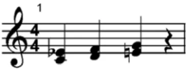
Figure 1.1: Polyphonic vs. Contrapuntal Interpretation
m:+:rest 0≡m
The operator (≡) should be read, “is musically equivalent to.” With this axiom it is easy to see that the original two expressions above are in fact musically equivalent.
For a more extreme example of this idea, and to entice the reader to learn more about musical equivalence in later chapters, note thatmel, given pitches p1 = Ef, p2 = F, p3 = G, and duration d = 1/4, generates the harmonized melody shown in Figure 1.1. One can write this concretely in Euterpea as:
mel1 = (note (1/4) (Ef,4) :=:note (1/4) (C,4)) :+: (note (1/4) (F, 4) :=:note (1/4) (D,4)) :+: (note (1/4) (G, 4) :=:note (1/4) (E,4))
The definition ofmel1can then be seen as apolyphonic interpretation of the musical phrase in Figure1.1, where each pair of notes is seen as a harmonic unit. In contrast, a contrapuntal interpretation sees two independent lines of notes, in this case the line E,F,G and the line C,D,E . In Euterpea one can write this as:
mel2 = (note (1/4) (Ef,4) :+:note (1/4) (F,4) :+:note (1/4) (G,4)) :=:
(note (1/4) (C, 4) :+:note (1/4) (D,4) :+:note (1/4) (E,4)) mel1 andmel2 are clearly not equal as Haskell values. Yet if they are played, they willsound the same—they are, in the sense described earlier, musically equivalent. But proving these two phrases musically equivalent will require far more than a simple axiom involving rest 0. In fact this can be done in an elegant way, using the algebra of music developed in Chapter11.
1.9
Code Reuse and Modularity
definition:
mel = (note qn p1:=:note qn (trans (−3)p1)) :+: (note qn p2:=:note qn (trans (−3)p2)) :+: (note qn p3:=:note qn (trans (−3)p3)) was replaced with:
mel =hList qn [p1,p2,p3]
But additionally, definitions for the auxiliary functionshNoteandhListwere introduced:
hNote ::Dur →Pitch→Music Pitch hNote d p =note d p:=:note d (trans (−3) p) hList ::Dur →[Pitch]→Music Pitch hList d [ ] =rest 0
hList d (p:ps) =hNote d p:+:hList d ps
In terms of code size, the final program is actually larger than the original! So has the program improved in any way?
Things have certainly gotten better from the standpoint of “removing re-peating patterns,” and one could argue that the resulting program therefore is easier to understand. But there is more. Now that auxiliary functions such as hNote and hList have been defined, one can reuse them in other contexts. Being able to reuse code is also calledmodularity, since the reused components are like little modules, or bricks, that can form the foundation of many applications.6 In a later chapter, techniques will be introduced—most notably,higher-order functions andpolymorphism—for improving the mod-ularity of this example even more, and substantially increasing the ability to reuse code.
1.10
[Advanced] Programming with Numbers
In computer music programming, it is often necessary to program with num-bers. For example, it is often convenient to represent pitch on a simple ab-solute scale using integer values. And when computing with analog signals that represent a particular sound wave, it is necessary to use floating point numbers as an approximation to the reals. So it is a good idea to under-stand precisely how numbers are represented inside a computer, and within a particular language such as Haskell.