Temporal Perspectives of Nonresponse During a Survey Design Phase

Temporal Perspectives of Nonresponse

During a Survey Design Phase

Taylor Lewis

U.S. Office of Personnel Management

Abstract

Invariably, full response is not achieved with a single survey solicitation, and so a sequence of follow-up attempts typically ensues in an effort to mitigate the potentially detrimental effects of nonresponse. Rather than permitting the follow-up campaign to continue indefi-nitely or until some preset response rate is met, a potentially more efficient alternative is to track a key point estimate in real-time as data is received and alter the survey design phase (i.e., modify the recruitment protocol) once the point estimate stabilizes. The notion of point estimate stability has been referred to as phase capacity in the survey methodology literature, and several methods to detect when it has occurred have been proposed in recent years. Noticeably absent from those works, however, is statistical theory providing insight into how point estimates can change during the course of data collection in the first place. The goal of this paper is to take a first step in developing that theory. To do so, the two es-tablished perspectives of survey nonresponse – deterministic and stochastic – are extended to account for the temporal dimension of responses obtained during a survey design phase. An illustration using data from the 2014 Federal Employee Viewpoint Survey is included to provide empirical support for the new theory introduced.

Keywords: responsive design, adaptive design, phase capacity, nonresponse bias, stopping rules

Acknowledgements

An earlier version of this article appeared as part of the author’s PhD dissertation “Test-ing for Phase Capacity in Surveys with Multiple Waves of Nonrespondent Follow-Up” from the Joint Program in Survey Methodology (JPSM) at the University of Maryland. The author would like to thank dissertation co-advisors Frauke Kreuter and Partha Lahiri for their encouragement, guidance, and feedback.

Disclaimer

The opinions, findings, and conclusions expressed in this article are those of the author and do not necessarily reflect those of the U.S. Office of Personnel Management.

Direct correspondence to

Taylor Lewis, U.S. Office of Personnel Management E-mail: [email protected]

1 Background

Unit nonresponse, which occurs whenever sampled cases (e.g., individuals, estab-lishments) fail to respond to a survey request, is a ubiquitous problem faced by practitioners. Indeed, evidence abounds that response rates have been declining in surveys worldwide (Atrostic et al., 2001; de Leeuw & de Heer, 2002; Curtin et al., 2005; Brick & Williams, 2013). The typical data collection protocol in a survey involves making a sequence of follow-up attempts on cases yet to respond, which can take on a variety of forms depending on the survey’s mode – reminder mailings, additional telephone calls, or revisits to a residence, to name a few. Each follow-up attempt generally yields more survey completes, which can be considered incom-ing waves of data. More follow-up attempts are ostensibly desirable, as they serve to reduce the nonresponse rate, but they can be costly and extend the field period, in turn delaying subsequent stages of the survey process, such as the reporting and analysis stages. And from a purely practical standpoint, empirical evidence (e.g., Table 1 in Potthoff et al., 1993; Table 1 in Lewis, 2017) suggests returns diminish with each subsequent wave; fewer and fewer completes are obtained, resulting in smaller and smaller changes in point estimates.

Rather than focusing on a target response rate or a predetermined number of completes, Groves & Heeringa (2006) advocate for the use of responsive survey design, which Schouten et al. (2013) note is a special case of adaptive survey design

incentive offered (McPhee & Hastedt, 2012), or terminating nonrespondent follow-up altogether (Rao et al., 2008). While being an intriguing idea that could poten-tially lead to data collection efficiencies, an obstacle to those wishing to implement their approach was that no specific, calculable rule was given regarding how to formally test for phase capacity. The concept was only demonstrated visually in Figure 2 of their paper in which they plotted the trend of a key National Survey of Family Growth point estimate.

Over the last ten or so years, several phase capacity testing methods have emerged in the literature. The first was Rao et al. (2008), who developed a set of closely related methods to determine whether the most recent wave of data pro-duced a statistically significant change in a sample mean. Lewis (2017) proposed a variant to their general approach amenable to any kind of point estimate, not strictly sample means. Wagner & Raghunathan (2010) took a prospective approach to testing for phase capacity, deriving a rule for determining whether or not a pend-ing follow-up attempt was necessary. In addition, Moore et al. (2016) proposed identifying phase capacity based on coefficient of variation thresholds of an overall and unconditional partial R-indicator (Schouten et al., 2009; Schouten et al., 2012). Noticeably absent in the works cited above is statistical theory to provide insight into the phenomenon of point estimate stability. That is, there is no theory offered to answer the following primordial question: How is it possible for a point estimate to change (or not change) over the course of a design phase? The works typically discuss the traditional nonresponse theory, but the traditional theory falls short because it is rooted in treating the act of responding as an all-or-nothing, yes-or-no event. In other words, the temporal dimension of the response process is not explicitly considered. This paper aims to fill that gap in the literature by extending the two traditional perspectives of nonresponse – deterministic and stochastic – to account for the timing of responses received during a survey design phase. Restrict-ing the focus to a sample mean, we derive expressions of expected change to be observed with each new wave of responses obtained. These expressions are enlight-ening and provide a theoretical underpinning for the empirical tendency for point estimates computed from the accumulating data to deviate less, relatively speaking, later on in a survey design phase (e.g., Figure 3 in Peytchev et al. 2009; Figure 3 in Wagner, 2010; Figure 1 in Lewis, 2017).

2 Traditional Nonresponse Perspectives

The typical survey’s data collection campaign commences by selecting a random sample of size n from a sampling frame constructed to represent all N units in a finite population. It has long been known from survey sampling theory that a ran-domly selected sample, even one of moderate size, can be used to form unbiased (or approximately unbiased) estimates of the attributes of the target population. The conundrum introduced by unit nonresponse is that, because only a portion of the sample is observed, unbiasedness properties are no longer guaranteed. Restricting analysis to the observed data without making any statistical adjustments may intro-duce nonresponse error (Groves, 1989), or a deviation from the quantity that would be computed had data been available for the full sample.

As discussed in Chapter 1 of Groves & Couper (1998), the magnitude of non-response error in a simple random sample of size n depends on both the statistic at hand and the degree of dissimilarity between the r observed cases and the m

missing cases (r + m = n). To consider one example, suppose we were interested in estimating a finite population mean

1

1 N i i

y y

N ₌

=

∑

. We can formulate an unbiased estimate from the full sample by finding

1

1 ˆ_n n _i

i

y y

n ₌

=

∑

. In the presence of unit non-response, however, we do not have all of the necessary information to compute this estimate. If we were to substitute

1 1

ˆ_r r _i

i

y y r ₌

=

∑

, the sample mean of the r observed

cases, as the estimate of the finite population mean, the nonresponse error would be

ˆ ˆ ˆ

( )NRerror y_r m (y_r y_m)

n

 

=_{  } − (1)

where

1 1

ˆ_m m _i

i

y y m ₌

=

∑

represents the mean of the m missing cases. In other words, nonresponse error is the product of the nonresponse rate and the difference in means between the observed and missing cases. Note, however, that in the presence of an unequal probability of selection sample design where each sampled case has been assigned a base weight equaling the inverse of its selection probability, one would need to substitute base-weighted versions of the two sample means in equa-tion 1. Addiequa-tionally, one would need to replace the term m/n with the base-weighted nonresponse rate.

been made (e.g., Lynn et al., 2002). To see this, suppose that the m nonrespondents in the sample are comprised of m_nc cases never contacted and m_ref cases who were reached but declined to participate in the survey (r + m_nc + m_ref = n). If we let_yˆ_nc

denote the mean of the m_nc cases never contacted and letyˆref denote the mean of

the m_ref cases refusing to participate, then the nonresponse error can be expressed as

ˆ ˆ ˆ ˆ ˆ

( ) (nc ) ref ( )

r m r nc m r ref

NRerror y y y y y

n n

= − + − (2)

Further decompositions of nonresponse error are possible, but the formulaic aug-mentation always abides by the same pattern: a new term is added representing the product of the prevalence of the group in the sample and the difference between the sample mean of the observed cases and the like for the group.

Lessler & Kalsbeek (1992) discuss at length the two traditional perspectives of nonresponse. The simpler view is the deterministic perspective, which stipulates that the N units on the sampling frame are comprised of two types: (1) a set of R

units that will always respond when sampled; and (2) a set of M units that will never respond. Under this view, Valliant et al. (2013, equation 13.1) report that the nonresponse bias is

ˆ

( )r M ( R M)

NRbias y y y N

 

=_{  } − (3)

whereyRrepresents the population mean of the units that always respond andyM

represents the like for units that never respond. Despite the resemblance to equa-tion 1, equaequa-tion 3 is expressed in terms of finite populaequa-tion quantities. In fact, the quantity in equation 1 can be considered an estimate of the quantity in equation 3.

An arguably more realistic view of nonresponse is the stochastic perspec-tive, which assumes instead that all units in the finite population have some prob-ability, or propensity, of responding to the survey request, a value between 0 and 1 frequently denoted ϕ_i. The concept and terminology are most often credited to Rosenbaum & Rubin (1983), but one can argue that the ideas trace back as far as Hartley (1946) and Politz & Simmons (1949). Given fixed propensities, if we let

1

1

φ φ

=

=

∑

N _i

i

N symbolize the average response propensity for all N population units,

Bethlehem (1988) showed that the nonresponse bias introduced by utilizingyˆr, the

sample mean for only the observed portion of the sample data, is approximately equal to

1

1 ˆ

( ) (φ φ)( )

φ ₌

≈

∑

N − −

r i i

i

NRbias y y y

which reveals how the bias is proportional to the population covariance of the propensities and the survey outcome variable. A preliminary result of the proof is that the expected value ofyˆrover the sampling and the nonresponse mechanisms

is 1

1

φ

φ =

=

∑

∑

N i i i

N i i

y

, which can be interpreted as the propensity-weighted mean of the

out-come variable in the population. Derivations appearing in the next section will make use of that result.

The expression in equation 4 attributable to Bethlehem (1988) can be related to the three missingness mechanisms defined by Little & Rubin (2002). The first is that data are missing completely at random (MCAR), which is to say that all units in the population share the same propensity, orφ φi = . In such a situation, there is no bias inyˆr, because the first term in the summation is 0. The second

mechanism, the one justifying most of the procedures used in practice to compen-sate for unit nonresponse, is that data are missing at random (MAR). Nonresponse adjustment techniques predicated on this mechanism exploit auxiliary data known for all sample units, both respondents and nonrespondents, such as information from the sampling frame or paradata. The MAR assumption permits response pro-pensities to vary amongst sample units with different auxiliary variable profiles, but supposes that the propensities are identical for all sample units with the same profile. Hence, data are assumed MCAR conditional on the sample units’ auxiliary variables. The third mechanism is the most perilous, data that are not missing at random (NMAR), meaning the sample units’ response propensities vary as a func-tion of the outcome variable beyond what can be explained (and adjusted for) by the auxiliary variables.

3 Alternative Nonresponse Perspectives to Frame

the Phase Capacity Problem

The purpose of this section is to introduce extensions to the traditional nonresponse perspectives outlined in the previous section. These extensions are motivated by the objective of providing theoretical insight into how a sample mean can change, and eventually stabilize, over the course of a survey design phase. Both the determinis-tic and stochasdeterminis-tic perspectives are considered.

A straightforward extension of the ideas behind the deterministic perspective of nonresponse for a survey collecting data over K waves is to conceptualize the N

always respond to the survey during the kth _{wave, and a domain of size M}

com-prised of units that will never respond. Because of the empirical tendency for the number of respondents to decrease with each subsequent follow-up attempt within a survey design phase (e.g., Table 1 in Potthoff et al., 1993; Table 1 in Lewis, 2017), it seems reasonable to expect the N_k’s to decrease in size as k increases.

Without loss of generality, as before, let us assume a simple random sample of size n has been selected and we are interested in making inferences on a finite pop-ulation mean. We can expect the wave-specific respondent counts r₁, r₂, …, r_K and the count of nonrespondents m (r₁ + r₂ + … + r_K + m = n) to fall approximately in proportion to their respective prevalences in the population – that is, E(r_k) = n(N_k/N) for k = 1, …, K and E(m) = n(M/N). Provided r_k > 1 for all K waves, we can express

the ultimate respondent sample mean as

1 ˆ ˆ k K k r r k r y y r =

=

∑

, where

1 K k k r r =

=

∑

andyˆr_k

represents the sample mean of the r_k cases responding during wave k, specifically. Following the same strategy used to partition nonresponse error in equation 2, we

can conceive of 1 1

1 ˆ ˆ j k j r j k k j j r y y r = = =

∑

∑

, the respondent mean using data from waves 1 to k

inclusive (k < K) (i.e., calculated using data from the r₁, r₂, …, r_k respondents thus far obtained) as susceptible to nonresponse error due to the fact that there have been

m nonrespondents drawn into the sample with meanyˆmthat will never respond and

* * 1 K k k k r = +

∑

cases that have yet to respond:

*

*

1 1 1 1

* 1

ˆ ˆ ˆ ˆ ˆ ˆ ˆ

( ) ( ) ( _k )

K

k k k k k

n m r

k k

r m

NRerror y y y y y y y n _{= +} n

= − = − +

∑

− (5)

We can consider 1 1

ˆ

y an estimate of 1 1

y , the mean of the population domain consisting of N₁ cases, and 2

1 ˆ

y an estimate of 2 1

y , the mean of the population domain consisting of N₁ + N₂ cases, and so on. In terms of conventional statistical hypothesis testing, methods to test for phase capacity, at least those described in Rao et al. (2008) and Lewis (2017), use the accumulating data to assess H₀:δkk−1=y1k−1−y1k =0 versus H₁: 1

1 1 1 0

k k k

k y y

δ −

− = − ≠ . Granted, the hypotheses can be written in terms of other

population parameters, and non-zero differences for that matter.

Note, however, that the difference specified in the hypotheses above can be re-expressed asδkk−1=(y1k−1−yn)−(y1k −yn), which reveals a parallel interpretation,

cumu-lative sample mean has not changed with the most recent wave of data set, then nonresponse bias has neither decreased nor increased.

The sample-based estimate ofδkk−1isδˆkk−1= yˆ1k−1−yˆ1k, which can be re-expressed as follows:

1

1 1 1

ˆk ˆk ˆk

k y y

δ −

− = −

1

1 1

ˆ ˆ ˆ ˆ

( k ) ( k )

n n

y − y y y

= − − −

1

1 1

ˆ ˆ

_{=NRerror y}( k−)_{−NRerror y}( )k

* *

1 * 1 *

1 1 1 1

* * 1

ˆ ˆ ˆ ˆ ˆ ˆ ˆ ˆ

( k ) K k ( k _k ) ( k ) K k ( k _k )

m r m r

k k k k

r r

m _{y y y y} m _{y y y y}

n n n n

− −

= = +

= − +

∑

− − − −

∑

−

* *

1 1 * 1

1 1 1 1 1

* 1

ˆ ˆ ˆ ˆ ˆ ˆ ˆ ˆ ˆ ˆ

( k k ) k ( k _k) K k ( k _k k _k )

m m r r r

k k

r r

m y y y y y y y y y y

n − n − _{= +} n −

 

= − − + + − +

∑

_ − − + _

1 * 1 1

1 1 1 1 1

* 1

ˆ ˆ ˆ ˆ ˆ ˆ

( k k) K k ( k k) k( k ) k k k

r r

m y y y y y y

n − _{= +} n − n −

 

= − +

∑

_ − _+ −

*

1 1

* 1

1 1 1

ˆ ˆ ˆ ˆ

( ) ( )

K k

k k k

k k k

k

m r

r

y y y y n= + − n −

  +     =_{ } − + −      

∑

(6)

which illustrates how the observed change in the sample mean is equal to the sum of two terms: (1) the product of the portion of sample cases yet to be observed fol-lowing wave k and the most recently observed change in the cumulative sample mean; and (2) the product of the portion of sample cases responding during wave k, specifically, and the difference between cumulative sample mean as of the previous wave and the sample mean of those responding during wave k. Because the r_k’s tend to decrease as k increases, we would expect both terms to get closer and closer to zero. With respect to the first term, this is becauseyˆ1kconsists of fewer and fewer

new values relative to 1 1 ˆk−

y , causing the difference_yk _yk 1 1

1 ˆ

ˆ − _{− to become smaller and}

smaller. With respect to the second term, this is because the multiplicative factor rK/n gets progressively smaller.

response process for the ith _{sample unit abides by a multinomial distribution with}

K + 1 events: responding during one of the K waves or not responding. Because all events are disjoint, we can treat the probability of responding by a particular wave as the sum of the entries in ϕ_i from the first position up to and including the entry indexing that wave. For example, the probability of the ith _{sample unit responding}

before or during wave k is 1 1 k k i ji j φ φ = =

∑

.

Alluded to earlier, a key preliminary result in the derivation of Bethlehem’s (1988) nonresponse bias formula is that, given a set of fixed response propensities, the expectation of the sample mean from any sample design is shown to equal

1 1 ˆ ( ) φ φ = = =

∑

∑

N i i i r N i i y

E y (7)

which is a weighted mean for all population units, where the response propensity serves as the weight. Using this result, we can reason that the expectation of the

sample mean at the first wave is

1

1 1

1 1 1

1 1 1 1 1 1 ˆ ( ) N N

i i i i

i i N N i i i i y y E y φ φ φ φ = = = = =

∑

=

∑

∑

∑

, and that the

expecta-tion of the sample mean at the second wave is

2 1 2 1 1 2 1 1 ˆ ( ) N i i i N i i y E y φ φ = = =

∑

∑

, and so on.

There-fore, we can express the expectation of the difference between two adjacent-wave sample means as

1

1 1

1 1 1

1 1 1 1 1 1 1 ˆ ˆ ( ) φ φ φ φ − − = = − = = − =

∑

−

∑

∑

∑

N N k k

i i i i

k k i i

N N

k k

i i

i i

y y

E y y (8)

This difference will only exactly equal zero if 1 1 1 1 1 1 1 1 N N k

i i ki i

i i N N k i ki i i y y φ φ φ φ − = = − = = =

∑

∑

increases, the ϕ_ki’s decrease, rendering the component of 1 1

N k

i i i

y

φ =

∑

attributable to

1

N ki i i

y

φ =

∑

to become smaller, and the same with the component of 1 1

N k

i i

φ =

∑

attribut-able to 1

φ =

∑

N ki i

. Hence, just as we could from the extended deterministic perspec-tive, we can extract theoretical justification from equation 8 for the empirical ten-dency of point estimate differences to get progressively smaller during a survey design phase.

4 Illustration in the 2014 Federal Employee

Viewpoint Survey

The purpose of this section is to provide an empirical illustration of the concepts and expressions presented in the previous section using data from the 2014 Fed-eral Employee Viewpoint Survey (FEVS) (www.fedview.opm.gov). The FEVS, for-merly known as the Federal Human Capital Survey (FHCS), was first launched in 2002 by the U.S. Office of Personnel Management (OPM). Initially administered biennially, the Web-based survey is now conducted yearly on a sample of full- or part-time, permanently employed civilian personnel of the U.S. federal government.

With few exceptions, the 2014 FEVS sampling frame was derived from a comprehensive personnel database managed by OPM known as the Statistical Data Mart of the Enterprise Human Resources Integration (EHRI-SDM). A total of 839,788 individuals from over 80 agencies were sampled as part of a single-stage stratified design, where strata were defined by the cross-classification of work unit and whether or not the employee was part of the Senior Executive Service (SES) or equivalent. The latter was done so that executives could be sampled with cer-tainty, as they represent a rare population domain of analytic interest. The work-unit stratification ensured adequate numbers of employees appeared in the sample for all pre-identified agency subdivisions for which a separate report was desired. For agencies with exceedingly intricate reporting needs, a census was conducted. See U.S. Office of Personnel Management (2014) for more details about the FEVS sampling methodology.

estimate from each item thus reduces to the proportion (or percentage) of employ-ees who react positively to the statement posed, what the FEVS administration team refers to as a “percent positive” statistic. For purposes of the present illustra-tion, we restrict the focus to percent positive statistics for the four items comprising the Global Satisfaction Index (GSI). These items were purposefully chosen because they represent a cross-section of the typical satisfaction dimensions the FEVS is designed to capture. The wording for the four items is summarized in Table 1.

The 2014 FEVS was administered between April 29 and June 13, 2014. Participat-ing agencies were given a choice of two possible start dates, April 29 or May 6. Each agency’s field period spanned six work weeks. At survey close, 392,752 completes had been obtained, corresponding to an overall response rate of 47.4% per formula RR3 of the American Association for Public Opinion Research (AAPOR) (2016).

With respect to the responsive survey design terminology attributable to Groves & Heeringa (2006), the 2014 FEVS data collection protocol can be consid-ered a single survey design phase. On the survey’s launch date, an email invitation containing the website URL and log-in credentials was sent to sampled employees. Five reminder emails were sent to those who had yet to respond, in weekly incre-ments thereafter. A final, sixth reminder was sent on Friday morning of the sixth field period week with messaging emphasizing that the survey would close at the end of the day. In all, seven email notifications were sent. A natural demarcation of a data collection wave, the one used in this illustration, is the set of responses obtained between two chronologically adjacent email notifications.

Table 2 summarizes the wave-specific respondent counts for one exam-ple agency participating in 2014 FEVS that conducted a census of its N = 5,188 employees. The greatest number of responses was obtained in the first wave, fol-lowed by the second wave, with returns diminishing in subsequent waves. A total of

m = 1,592 employees never responded, even after being sent seven email notifica-tions. Though not shown here, comparable patterns hold for most other participat-ing agencies. Thinkparticipat-ing back to the second term of equation 6, this lends empirical

Table 1 2014 Federal Employee Viewpoint Survey Items Comprising the Global Satisfaction Index

Item

Number Wording

credence to the assertion of the r_k terms decreasing as k increases, a major factor in the stabilization of a sample mean over the course of a survey design phase.

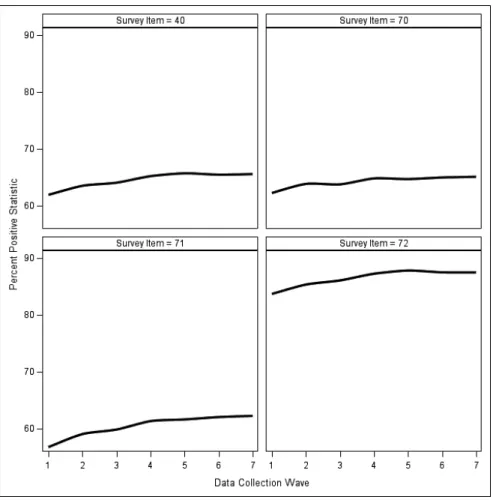
The decreasing r_k’s also factor implicitly into the first product in equation 6, as is evident from Figure 1, which plots the trends in the cumulative sample means of the four GSI items using responses obtained through the given wave (i.e., the

1

ˆk

y ’s) for the example agency. The cumulative means tend to increase with each new wave of data, at least for the early waves, but then stabilize around wave 5. The increasing pattern is an indication that the early responders are less positive than later responders, something Sigman et al. (2014) noted was widespread amongst agencies participating in the 2011 FEVS.

With respect to the stochastic perspective of nonresponse, recall the primary takeaway argument from equation 8 was that, because the wave-specific propensi-ties (i.e., the ϕ_ki’s) tend to decrease as k increases, the component of 1

1 φ =

∑

N k i i

attrib-utable to

1

N ki i

φ =

∑

and the component of 1

1 φ =

∑

N k i i i

y attributable to 1

N ki i i

y

φ =

∑

should both

become progressively smaller over the course of a design phase. When those respec-tive components of the summations become negligible, phase capacity results.

To illustrate how this can happen, we can exploit information from the 2014 FEVS sampling frame. Specifically, using auxiliary information known for the entire population of N = 5,188 individuals in the agency, we utilized the employee’s age, gender, an indicator of being a supervisor/non-supervisor, an indicator of being minority/non-minority race or ethnicity, and an indicator of working in the head-quarters or field office, to fit a multinomial logistic regression model where the outcome variable was one of 8 possible events: responding during wave 1, 2, …, 7,

Table 2 Wave-Specific Response Distribution for an Example Agency Participating in the 2014 Federal Employee Viewpoint Survey

Data Collection Wave

k Count r_k Percent of Sample (r_k / n) * 100

1 1,390 26.8

2 873 16.8

3 240 4.6

4 392 7.6

5 246 4.7

6 260 5.0

7 195 3.8

Nonrespondents 1,592 30.7

or not responding at all. This model was used to generate estimated wave-specific propensities, orφˆki’s, which can serve as substitutes for the ϕki’s.

Table 3 reports the proportions 1 1

1 1

ˆ _/ ˆ

φ φ

= =

∑ ∑

N N k

i i

i i

and 1 1

1 1

ˆ _/ ˆ

N N

k i ki i ki

i i

y y

φ φ

= =

∑

∑

for the

four GSI items, where y_ki is an indicator variable equaling 1 for a positive response to a given item and 0 otherwise. Each of these proportions converges towards zero, which is to say that both the numerator and denominator terms of the expected value of the cumulative sample mean (see equation 8) change less and less. By wave 5, the proportional change is less than 10%, suggesting an ineffectual impact, which coincides with the point estimate stabilization observed in Figure 1.

5 Discussion

Faced with downward pressures on response rates, practitioners must nowadays explore alternative strategies to more effectively and efficiently manage a survey’s data collection process. One intuitive method for doing so is to monitor a key point estimate from the survey in real-time as completes are obtained and take note of when it stabilizes. This is the notion of phase capacity, as defined by Groves & Hee-ringa (2006), who argue that additional follow-up efforts are liable to be equally inefficacious. Instead, some form of change in the data collection protocol is war-ranted. In their terminology, a new design phase is in order.

Groves & Heeringa (2006) did not offer a formal method to test for phase capacity, but several techniques have since been proposed in the literature (Rao et al., 2008; Wagner & Raghunathan, 2010; Moore et al., 2016; Lewis, 2017). An important piece missing from those proposals, however, is statistical theory illu-minating how (or when) point estimate changes could occur in the first place. The objective of this paper was to fill that void in the literature. Using the finite popula-tion mean as an example, we extended the tradipopula-tional deterministic and stochastic perspectives of nonresponse to derive expressions of change that explicitly account for incoming waves of responses within a single design phase. To connect these ideas to practice and to secure empirical support of certain assumptions and asser-tions made during the derivaasser-tions, we included an illustration using data from the

Table 3 Proportions of Estimated Wave-Specific Response Propensities, and Proportions of the Products of Estimated Wave-Specific Response Propensities with GSI Positive/Non-Positive Indicator Variables for an Example Agency Participating in the 2014 Federal Employee Viewpoint Survey

Data Collection Wave

k Propensities Propensities x Item 40

Propensities

x Item 70 Propensities x Item 71 Propensities x Item 72

1 1.00 1.00 1.00 1.00 1.00

2 0.39 0.39 0.38 0.39 0.39

3 0.10 0.10 0.10 0.10 0.10

4 0.14 0.14 0.13 0.14 0.14

5 0.08 0.08 0.08 0.08 0.08

6 0.08 0.08 0.07 0.08 0.08

2014 Federal Employee Viewpoint Survey. In particular, focusing on four survey items for one example agency, we showed how the stabilization occurring around the fifth wave of data received was largely a function of the decreasing respondent counts (i.e., the r_k’s in equation 6) and the associated decreasing (estimated) wave-specific propensities that factor into the two quotients in equation 8.

Of course, this paper is not without limitations. The first limitation is that we focused solely on a sample mean. Brick & Jones (2008) derive expressions of nonresponse bias for several other statistics. Modifications to those expressions accounting for the temporal dimension of nonresponse could have proven equally as enlightening. A second limitation is that, for tractability, the derivations pre-sented in Sections 2 and 3 assumed no nonresponse adjustments have been made. In fact, the phase capacity testing methods proposed in Rao et al. (2008), Wagner & Raghunathan (2010), and Lewis (2017) call for nonresponse adjustments to be made prior to assessing whether point estimate stability has occurred. A third limi-tation is that the 2014 FEVS illustration only involved analysis of four survey items for one example agency. Although we argued that the patterns observed are very typical for the FEVS, both in terms of other items’ percent positive statistics and other participating agencies, it is certainly conceivable that a comparable illustra-tion within the design phase(s) of another survey could yield results less harmoni-ous with the nonresponse theory extended in this paper.

References

American Association for Public Opinion Research (AAPOR). (2016). Standard definitions: Final dispositions of case codes and outcome rates for surveys (9th _{edition). AAPOR.} Atrostic, B., Bates, N., Burt, G., & Silberstein, A. (2001). Nonresponse in US government

household surveys: Consistent measures, recent trends, and new insights. Journal of Official Statistics, 17 (2), 209-226.

Bethlehem, J. (1988). Reduction of nonresponse bias through regression estimation. Journal of Official Statistics, 4 (3), 251-260.

Brick, M., & Jones, M. (2008). Propensity to respond and nonresponse bias. Metron-Inter-national Journal of Statistics, 66 (1), 51-73.

Brick, M., & Williams, D. (2013). Explaining rising nonresponse rates in cross-sectional surveys. ANNALS of the American Academy of Political and Social Science, 645 (1), 36-59.

Couper, M. (1998). Measuring survey quality in a CASIC environment. Paper presented at the Joint Statistical Meetings of the American Statistical Association.

Curtin, R., Presser, S., & Singer, E. (2005). Changes in telephone survey nonresponse over the past quarter century. Public Opinion Quarterly, 69 (1), 87-98.

de Leeuw, E., & de Heer, W. (2002). Trends in household survey nonresponse: A longitu-dinal and international comparison. In R. Groves, D. Dillman, J. Eltinge, & R. Little (Eds.), Survey Nonresponse, New York: Wiley.

de Leeuw, E. (2005). To mix or not to mix data collection modes in surveys. Journal of Official Statistics, 21 (2), 233-255.

Groves, R. (1989). Survey errors and survey costs. New York: Wiley.

Groves, R., & Couper, M. (1998). Nonresponse in household interview surveys. New York: Wiley.

Groves, R., & Heeringa, S. (2006). Responsive design for household surveys: tools for ac-tively controlling survey errors and costs. Journal of the Royal Statistics Society: Se-ries A, 169 (3), 439-457.

Hartley, H. (1946). Discussion of “A review of recent statistical developments in sampling and sampling surveys” by Yates, F. Journal of the Royal Statistical Society: Series A, 109 (1), pp. 37-38.

Kreuter, F. (2013). Improving surveys with paradata: Analytic uses of process information. Hoboken: Wiley.

Lessler, J., & Kalsbeek, W. (1992). Nonsampling error in surveys. New York: Wiley. Lewis, T. (2017). Univariate Tests for Phase Capacity: Tools for Identifying When to Modify

a Survey’s Data Collection Protocol. Journal of Official Statistics (in press).

Little, R., & Rubin, D. (2002). Statistical analysis with missing data (2nd _{edition). New York:} Wiley.

Lynn, P., Clarke, P., Martin, J., & Sturgis, P. (2002). The effects of extended interviewer effort on nonresponse bias. In R. Groves, D. Dillman, J. Eltinge, & R. Little (Eds.),

Survey Nonresponse, New York: Wiley.

Moore, J., Durrant, G., & Smith, P. (2016). Data set representativeness during data collec-tion in three UK social surveys: Generalizability and the effects of auxiliary covariate choice. Journal of the Royal Statistics Society: Series A, online first edition.

Olson, K., & Groves, R. (2012). An examination of within-person variation in response pro-pensity over the data collection field period. Journal of Official Statistics, 28 (1), 29-51. Peytchev, A., Baxter, R., & Carley-Baxter, L. (2009). Not all survey effort is equal: Re-duction of nonresponse bias and nonresponse error. Public Opinion Quarterly, 73 (4), 785-806.

Politz, A., & Simmons, W. (1949). An attempt to get the not-at-homes into the sample wit-hout callbacks. Journal of the American Statistical Association, 44 (245), 9-31. Potthoff, R., Manton, K., & Woodbury, M. (1993). Correcting for nonavailability bias in

surveys by weighting based on the number of callbacks. Journal of the American Stati-stical Association, 88 (424), 1197-1207.

Rao, R., Glickman, M., & Glynn, R. (2008). Stopping rules for surveys with multiple waves of nonrespondent follow-up. Statistics in Medicine, 27 (12), 2196-2213.

Rosenbaum, P., & Rubin, D. (1983). The central role of the propensity score in observational studies for causal effects. Biometrika, 70 (1), 41-55.

Schouten, B., Cobben, F. & Bethlehem, J. (2009). Indicators for the representativeness of survey response. Survey Methodology, 35 (1), 101-113.

Schouten, B., Bethlehem, J., Beullens, K., Kleven, Ø., Loosveldt, G., Luiten, A., Rutar, K., Shlomo, N. & Skinner, C. (2012). Evaluating, comparing, monitoring, and improving representativeness of survey response through R-indicators and partial R-indicators.

International Statistical Review, 80 (3), 382-399.

Schouten, B., Calinescu, M. & Luiten, A. (2013). Optimizing quality of response through adaptive survey designs. Survey Methodology, 39 (1), 29-58.

Sigman, R., Lewis, T., Yount Dyer, N., & Lee, K. (2014). Does the length of fielding period matter? Examining response scores of early versus late responders. Journal of Official Statistics, 30 (4), 651-674.

United States Office of Personnel Management. (2014). Federal employee viewpoint survey results: Technical report. Retrieved September 13, 2016 from the Federal Employee Viewpoint Survey website: http://www.fedview.opm.gov/2014/published/.

Valliant, R., Dever, J., & Kreuter, F. (2013). Practical tools for designing and weighting survey samples. New York: Springer.

Wagner, J. (2008). Adaptive survey design to reduce nonresponse bias. Ph.D. thesis, Univer-sity of Michigan.

Wagner, J. (2010). The fraction of missing information as a tool for monitoring the quality of survey data. Public Opinion Quarterly, 74 (2), 223-243.